hep-ph/0501086 DFPD-05/TH/01

Proton Lifetime from SU(5) Unification
in Extra Dimensions

Maria Laura Alciati     Ferruccio Feruglio 

Dipartimento di Fisica ‘G. Galilei’, Università di Padova

INFN, Sezione di Padova, Via Marzolo 8, I-35131 Padua, Italy

Yin Lin  and Alvise Varagnolo 

Scuola Normale Superiore, Pisa

INFN, Sezione di Pisa, I-56126 Pisa, Italy

We provide detailed estimates of the proton lifetime in the context of simple supersymmetric SU(5) grand unified models with an extra compact spatial dimension, described by the orbifold $S^{1}/(Z_{2}\times Z_{2}^{\prime})$ and by a large compactification scale $M_{c}\approx 10^{14}\div 10^{16}$ GeV. We focus on a class of models where the grand unified symmetry is broken by the compactification mechanism and where baryon violation proceeds mainly through gauge vector boson exchange so that the proton lifetime scales as $M_{c}^{4}$. We carefully compute $M_{c}$ from a next-to-leading analysis of gauge coupling unification and we find that $M_{c}$ can only be predicted up to an overall factor $10^{\pm 1}$. The simplest model, where the dominant decay mode is $\pi^{0}e^{+}$ and has no flavour suppression, is strongly constrained by existing data, but not totally ruled out. We also analyze models where some of the matter fields are localized in the extra space and proton decay is flavour suppressed. In models associated to anarchy in the neutrino sector the preferred decay channel is $K^{+}{\bar{\nu}}$ and the lifetime can be within the reach of the next generation of experiments.

1 Introduction

Grand unification can be considered a cornerstone in our quest for unification of particle interactions. Many properties of the standard model of electroweak and strong interactions that seem mysterious or accidental, like the particle content, the cancellation of gauge anomalies, the quantization of the electric charge, appear natural in the context of grand unified theories (GUTs). The quantitative success of gauge coupling unification in supersymmetric (SUSY) GUTs is remarkable and the vicinity of the GUT scale to the Planck scale is quite intriguing. Also the observed smallness of neutrino masses, suggesting the breaking of the total lepton number L at very high energies, supports the idea of a new threshold in particle physics at the GUT scale.

Despite the attractiveness of the GUT idea and its influence in both theoretical and experimental developments, proton decay, that represents its most characteristic prediction, has eluded all the experimental searches so far. Stringent limits on the proton lifetime in many channels have been set, such as [1]

$$\tau(p\to\pi^{0}e^{+}) > 5.4\times 10^{33}~{}{\rm yr}~{}~{}~{}~{}~{}~{}~{}90\%{\rm C.L.}$$

$$\tau(p\to K^{+}{\bar{\nu}}) > 2.2\times 10^{33}~{}{\rm yr}~{}~{}~{}~{}~{}~{}~{}90\%{\rm C.L.}$$ (1)

and, as a consequence, the minimal SUSY GUTs are tightly constrained or even ruled out. The proton decay rate in minimal SUSY GUTs depends on many parameters and there are many sources of theoretical uncertainties, such as the mass of the colour triplets whose exchange dominates the amplitudes, the hadronic matrix elements, the spectrum of SUSY particles, $\tan\beta$, unknown phases and mixing angles from the flavour sector. Even by stretching the uncertainties to their limits, minimal SUSY SU(5) is already ruled out by now [2] and, in general, only non-minimal schemes, considerably more complicated than the minimal ones, survive this important test [3]. On the theoretical side a related difficulty of minimal GUTs is how to reconcile light electroweak doublets with superheavy colour triplets, both occurring in the same GUT multiplets: the so-called doublet-triplet splitting problem. In minimal GUTs such a splitting is achieved through a fine-tuning by fourteen orders of magnitude. Even when such a splitting is obtained, either by fine-tuning or by another mechanism, in many models it is upset by radiative corrections when SUSY is broken and/or by non-renormalizable operators which can originate from the physics at the cut-off scale [4].

An appealing mechanism to achieve the desired splitting is when the grand unified symmetry is broken by the compactification mechanism in models with extra spatial dimensions [5]. In the last years this mechanism has been reproduced in the context of simple field theoretical models, GUTs defined in five or more space-time dimensions [6]. In the simplest case a single extra spatial dimension is compactified on a circle. The Lagrangian of the theory is invariant under SU(5), but the fields are periodic only up to transformations leaving the SU(5) algebra invariant. This requirement produces automatically a mass splitting in complete SU(5) multiplet. For instance, in the gauge vector boson sector, the only fields that remain massless correspond to the vector bosons of the standard model. All the other states, including the extra gauge bosons $X$ of SU(5), become massive, with masses of the order of the compactification scale $M_{c}\equiv 1/R$. This is a simple and elegant way to effectively break SU(5) down to the standard model gauge group. The same boundary conditions that break the grand unified symmetry should be consistently extended to the other fields of the theory and in particular to the multiplet containing the electroweak doublets and colour triplets. As a consequence, an automatic doublet-triplet splitting of order $1/R$ occurs, with no need of an ad hoc scalar sector.

It has soon been realized that such a framework has interesting consequences also on the prediction of proton lifetime. Proton could even be made stable in such a construction [7, 8]. In a less radical approach, the automatic doublet-triplet splitting is accompanied by the absence of baryon-violating dimension five operators [9]. Therefore proton decay can only proceed through dimension six operators, originating from the exchange of the superheavy gauge vector bosons $X$ between the ordinary fermions. In conventional, four-dimensional models, the inverse decay rate due to dimension six operators is given by [10]

$$\tau(p\to\pi^{0}e^{+})=1.6\times 10^{36}~{}{\rm yr}\times\left(\frac{\alpha~{}({\rm GeV}^{3})}{0.015}\right)^{-2}\times\left(\frac{\alpha_{U}}{1/25}\right)^{-2}\times\left(\frac{M_{X}~{}({\rm GeV})}{2\times 10^{16}}\right)^{4}~{}~{}~{},$$ (2)

where $M_{X}$ is the mass of the gauge vector bosons $X$, $\alpha_{U}$ is the gauge coupling constant at the unification scale and $\alpha$ is a parameter coming from the evaluation of the hadronic matrix element. The central value in (2) is too large to be observed, even by the next generation of experiments. In five dimensional models there are important modifications and the prediction, even in the most conservative case, can be quite different from the one in (2). First the proton lifetime scales with the fourth power of the compactification scale $M_{c}$, which can be considerably smaller than the central value of $M_{X}$ in eq. (2). Second, the coupling of the gauge vector bosons $X$ to ordinary fermions differs, in general, from four-dimensional SUSY SU(5). This has to do with the freedom of introducing matter fields either as ‘bulk’ fields, depending on the extra spatial dimension, or as ‘brane’ fields, localized in a particular four-dimensional subspace of the full space-time.

In this paper we focus on the five-dimensional SUSY SU(5) GUT described in ref. [9, 11, 12], which can be considered among the simplest realizations of GUTs in extra dimensions . There are estimates of the proton decay rate in this model and its variants. In ref. [9, 11] the compactification scale $M_{c}$ has been evaluated from the analysis of gauge coupling unification in a leading order approximation. By calling $\Lambda$ the cut-off scale of the theory, it has been shown that, for $\Lambda R$ equal to 100 (10), the compactification scale ranges in

$$5\times 10^{14}~{}(3\times 10^{15})~{}{\rm GeV}\leq M_{c}\leq 2\times 10^{15}~{}(8\times 10^{15})~{}{\rm GeV}~{}~{}~{}.$$ (3)

Indeed $\Lambda R\approx 100$ is preferred by a more refined estimate [14] and, if we naively substitute $2M_{c}/\pi$ to $M_{X}$ in eq. (2), we find a proton lifetime

$$1.0\times 10^{29}~{}{\rm yr}\leq\tau(p\to\pi^{0}e^{+})\leq 2.6\times 10^{31}~{}{\rm yr}~{}~{}~{},$$ (4)

already excluded by the experimental bound of eq. (1). In this first estimate, however, it has been assumed that all matter fields are coupled to the $X$ bosons as in the four-dimensional theory. Actually, a more suitable setting for a natural interpretation of the fermion mass hierarchies requires that only $T_{3}$ and $F_{i}$ $(i=1,2,3)$ couple to the $X$ boson as in the four-dimensional theory [11, 12, 15]. Here $T$ and $F$ denote 10 and ${\bar{5}}$ SU(5) representations and the index labels the different generations. In such a framework the leading baryon-violating dimension six operator is $T^{\dagger}_{3}T_{3}F^{\dagger}_{1}F_{1}$. Mixing angles are required to convert third generation fields into states relevant to proton decay and the amplitude for the dominant decay mode, $K^{+}{\bar{\nu}}$, is depleted by $\lambda^{5}$ with respect to $\pi^{0}e^{+}$ in the four-dimensional theory, $\lambda\approx 0.22$ being a Cabibbo suppression factor. The conclusion of ref. [12] is that

$$\tau(p\to K^{+}{\bar{\nu}})\approx 10^{37\pm 2}~{}{\rm yr}~{}~{},$$ (5)

unless additional, model dependent contributions are invoked.

The result (5) is not far from the expected sensitivity of future Water Cerenkov and Liquid Argon detectors for the $K^{+}{\bar{\nu}}$ mode [16]:

$$0.2\times 10^{35}~{}{\rm yr} ~{}~{}~{}~{}~{}~{}~{}~{}~{}{\rm 10yr,650kton}~{}~{}~{}~{}~{}~{}~{}~{}~{}~{}{\tt Water~{}Cherenkov}$$

$$1.1\times 10^{35}~{}{\rm yr} ~{}~{}~{}~{}~{}~{}~{}~{}~{}{\rm 10yr,100kton}~{}~{}~{}~{}~{}~{}~{}~{}~{}~{}{\tt Liquid~{}Argon}$$ (6)

This strongly motivates a careful and complete quantitative estimate of the proton lifetime in this model, with a particular attention to the main sources of theoretical uncertainties, that can sizeably affect the estimate in eq. (5). Such an analysis is the purpose of this paper. First of all we compute $M_{c}$ from a next-to-leading analysis of gauge coupling unification, including two-loop running, threshold corrections from SUSY particles, and possible SU(5) breaking contributions allowed by the present construction. As we will see in detail in section 4, we find that there is a big theoretical uncertainty on $M_{c}$, entirely dominated by the expected SU(5)-breaking contributions and not accounted for by the previous estimates. According to our analysis $M_{c}$ can range from approximately $10^{14}~{}{\rm GeV}$ to more than $10^{16}~{}{\rm GeV}$, a considerably wider interval than in eq. (3). We also size the uncertainty coming from the flavour sector, by contemplating different settings for matter fields. In what we call ‘option 0’, all matter fields are coupled to the $X$ gauge bosons as in four-dimensional SUSY SU(5). We will also consider two other possibilities, that we call ‘option I’ and ‘option II’. Option II corresponds to $T_{3}$ and $F_{i}$ $(i=1,2,3)$ coupled to $X$ as in four dimensions, whereas in option I only $T_{3}$ and $F_{3,2}$ have standard couplings. As far as neutrino mass matrices are concerned, option I and option II give rise to “semianarchy” and “anarchy”, respectively [17]. We estimate the degree of flavour suppression by counting powers of the Cabibbo angle $\lambda$, in two different ways, characterized by a stronger and a milder mixing between the different generations. This allows us to estimate also the theoretical uncertainty coming from the Yukawa sector.

Our results are presented in section 5. They are qualitatively different for option 0 and options I/II. In option 0, the dominant decay mode is $\pi^{0}e^{+}$ and the lifetime is obtained from eq. (2) through the substitution $M_{X}\to 2M_{c}/\pi$ . Due to the large uncertainty on $M_{c}$ we will see that such an option is strongly constrained, but not totally ruled out. In option I and II, we confirm that $K^{+}{\bar{\nu}}$ is one of the dominant decay channels. The prospects for detectability of proton decay in this channel by future machines are good, but only with favorable combinations of mixing angles (option II is needed) and of SU(5)-violating terms at the cut-off scale. We also evaluate branching ratios for proton decay, much less affected by uncertainties than absolute rates.

2 SU(5) unification in extra dimensions

2.1 Space-time orbifold

Following ref. [6] we consider a 5-dimensional space-time factorized into a product of the ordinary 4-dimensional space-time M₄ and of the orbifold $S^{1}/(Z_{2}\times Z_{2}^{\prime})$, with coordinates $x^{\mu}$, ($\mu=0,1,2,3$) and $y=x^{5}$. The orbifold $S^{1}/(Z_{2}\times Z_{2}^{\prime})$ is obtained from the circle $S^{1}$ of radius $R$ with the identification provided by the two reflections:

$$Z_{2}:~{}~{}~{}~{}~{}~{}~{}~{}~{}~{}y\rightarrow-y~{}~{}~{}~{}~{},$$ (7)

$$Z_{2}^{\prime}:~{}~{}~{}~{}~{}~{}~{}~{}~{}y^{\prime}\rightarrow-y^{\prime}~{}~{}~{}~{}~{}(y^{\prime}\equiv y-\pi R/2)~{}~{}~{}~{}~{}.$$ (8)

As a fundamental region of the orbifold, we can take the interval from $y=0$ to $y=\pi R/2$. At the two sides of the interval, we have two four-dimensional boundaries of the space-time, called branes. On the covering space, $S^{1}$, where we choose to work from now on, the origin $y=0$ and $y=\pi R$ represent the same physical point and similarly for $y=+\pi R/2$ and $y=-\pi R/2$. When speaking of the brane at $y=0$, we actually mean the two four-dimensional slices at $y=0$ and $y=\pi R$, and similarly $y=\pi R/2$ stands for both $y=\pm\pi R/2$.

For a generic field $\phi(x^{\mu},y)$ living in the 5-dimensional bulk the $Z_{2}$ and $Z_{2}^{\prime}$ parities $P$ and $P^{\prime}$ are defined by

$$\phi(x^{\mu},y) \to\phi(x^{\mu},-y)=P\phi(x^{\mu},y)~{}~{}~{},$$

$$\phi(x^{\mu},y^{\prime}) \to\phi(x^{\mu},-y^{\prime})=P^{\prime}\phi(x^{\mu},y^{\prime})~{}~{}~{}.$$ (9)

Denoting by $\phi_{\pm\pm}$ the fields with $(P,P^{\prime})=(\pm,\pm)$ we have the $y$-Fourier expansions:

$$\phi_{++}(x^{\mu},y) = \sqrt{1\over{2\pi R}}\phi^{(0)}_{++}(x^{\mu})+\sqrt{1\over{\pi R}}\sum_{n=1}^{\infty}\phi^{(2n)}_{++}(x^{\mu})\cos{2ny\over R}~{}~{}~{},$$

$$\phi_{+-}(x^{\mu},y) = \sqrt{1\over{\pi R}}\sum_{n=0}^{\infty}\phi^{(2n+1)}_{+-}(x^{\mu})\cos{(2n+1)y\over R}~{}~{}~{},$$

$$\phi_{-+}(x^{\mu},y) = \sqrt{1\over{\pi R}}\sum_{n=0}^{\infty}\phi^{(2n+1)}_{-+}(x^{\mu})\sin{(2n+1)y\over R}~{}~{}~{},$$

$$\phi_{--}(x^{\mu},y) = \sqrt{1\over{\pi R}}\sum_{n=0}^{\infty}\phi^{(2n+2)}_{--}(x^{\mu})\sin{(2n+2)y\over R}~{}~{}~{}.$$ (10)

where $n$ is a non negative integer and the notation is such that the Fourier component field $\phi^{(n)}(x)$ acquires a mass $n/R$ upon compactification. Only $\phi_{++}$ has a massless component and only $\phi_{++}$ and $\phi_{+-}$ are non-vanishing on the $y=0$ brane. The fields $\phi_{++}$ and $\phi_{-+}$ are non-vanishing on the $y=\pi R/2$ brane, while $\phi_{--}$ vanishes on both branes. The normalization is such that:

$$\int_{-\pi R}^{+\pi R}dy|\phi(x,y)|^{2}=\sum_{n=0}^{\infty}|\phi^{(n)}(x)|^{2}~{}~{}~{}.$$ (11)

2.2 Gauge and Higgs sectors

The theory under investigation, defined in the above five-dimensional space-time, is invariant under N=1 SUSY, which corresponds to N=2 in four dimensions, and under SU(5) gauge transformations. We can keep working in the entire circle if we also ask invariance under $Z_{2}\times Z_{2}^{\prime}$ parities. The parities of the fields are assigned in such a way that compactification reduces N=2 to N=1 SUSY and breaks SU(5) down to the SM gauge group ${\rm SU(3)}\times{\rm SU(2)}\times{\rm U(1)}$. Leaving aside for the moment quarks and leptons and their SUSY partners, the 5-dimensional theory contains the following N=2 SUSY multiplets of fields. First, a vector multiplet with vector bosons $A_{M}$, $M=0,1,2,3,5$, two bispinors $\lambda^{i}$, $i=1,2$, and a real scalar $\Sigma$, each of them transforming as a 24 representation of SU(5).

$(P,P^{\prime})$	field	mass
$(+,+)$	$A^{a}_{\mu}$, $\lambda^{2a}$, $H^{D}_{u}$, $H^{D}_{d}$	$\frac{2n}{R}$
$(+,-)$	$A^{\hat{a}}_{\mu}$, $\lambda^{2\hat{a}}$, $H^{T}_{u}$, $H^{T}_{d}$	$\frac{(2n+1)}{R}$
$(-,+)$	$A^{\hat{a}}_{5}$, $\Sigma^{\hat{a}}$, $\lambda^{1\hat{a}}$, $\hat{H}^{T}_{u}$, $\hat{H}^{T}_{d}$	$\frac{(2n+1)}{R}$
$(-,-)$	$A^{a}_{5}$, $\Sigma^{a}$, $\lambda^{1a}$, $\hat{H}^{D}_{u}$, $\hat{H}^{D}_{d}$	$\frac{(2n+2)}{R}$

Table 1: Parity assignment and masses ($n\geq 0$) of fields in the vector and Higgs supermultiplets.

These fields can be arranged in an N=1 vector supermultiplet $V\equiv(A_{\mu},\lambda^{2})$ and an N=1 chiral multiplet $\Phi\equiv(A_{5},\Sigma,\lambda^{1})$, both transforming in the adjoint representation of SU(5). Then there are two hypermultiplets $H^{s}$ ($s=1,2$), each of them consisting of two N=1 chiral multiplets: $H^{1}=(H_{5},\hat{H}_{\bar{5}})$ and $H^{2}=(H_{\bar{5}},\hat{H}_{5})$. Here $H_{5}$ and $H_{\bar{5}}$ stand for the usual SU(5) supermultiplets, which include the scalar Higgs doublets $H^{D}_{u}$ and $H^{D}_{d}$ and the corresponding scalar triplets $H^{T}_{u}$ and $H^{T}_{d}$, respectively. The other two, $\hat{H}_{\bar{5}}$ and $\hat{H}_{5}$, transform as $\bar{5}$ and 5, under SU(5). The parity $P$, $P^{\prime}$ assignments are the same as in ref. [6] and are given in table 1.

Here the index $a$ ($\hat{a}$) labels the unbroken (broken) SU(5) generators $T^{a}$ ($T^{\hat{a}}$), $H$ stands for the whole chiral multiplet of given quantum numbers. The parity $P$ breaks N=2 SUSY down to N=1 and would allow complete SU(5) massless supermultiplets, contained in the first two rows of table 1. The additional parity $P^{\prime}$ respects the surviving N=1 SUSY and breaks SU(5) down to the standard model gauge group. Note that the derivative $\partial_{5}$ transforms as $(-,-)$. The $(+,+)$ fields, which remain massless and do not vanish on both branes are the gauge and Higgs multiplets of the low energy Minimal SUSY Model (MSSM). The bulk 5-dimensional Lagrangian is exactly as in ref. [6] and we do not reproduce it here.

The vector bosons $A_{\mu}^{a(0)}$ remain massless and, together with the gauginos $\lambda^{2a(0)}$, form a vector supermultiplet of N=1. All the other vector bosons are massive and become component of N=1 massive vector supermultiplets. Therefore the SU(5) gauge symmetry is effectively broken down to SU(3) $\times$ SU(2) $\times$ U(1) and the symmetry breaking order parameter is the inverse radius $1/R$, which is expected to be of the order of the unification scale. At the same time, in the Higgs sector, only the Higgs doublets and their superpartners are massless, while colour triplets and extra states acquire masses of order $1/R$, giving rise to an automatic doublet-triplet splitting. The N=2 SUSY algebra would allow a mass term between the hypermultiplets $H^{1}$ and $H^{2}$ [18], thus spoiling the lightness of the Higgs doublets achieved by compactification, but such a term can be forbidden by explicitly requiring an additional U(1)_R symmetry [9, 12]. This U(1)_R symmetry is the diagonal subgroup of an $R$-symmetry acting on the Higgs multiplets as

$$(H_{5},\hat{H}_{\bar{5}})^{\prime}(\theta) = e^{i\alpha}(H_{5},\hat{H}_{\bar{5}})(e^{-i\alpha}\theta)$$ (12)

$$(H_{\bar{5}},\hat{H}_{5})^{\prime}(\theta) = e^{i\alpha}(H_{\bar{5}},\hat{H}_{5})(e^{-i\alpha}\theta)~{}~{}~{}$$ (13)

and a U(1) symmetry acting as:

$$(H_{5},{\hat{H}_{\bar{5}}}^{\dagger})^{\prime} = e^{-i\alpha}(H_{5},{\hat{H}_{\bar{5}}}^{\dagger})$$ (14)

$$(H_{\bar{5}},{\hat{H}_{5}}^{\dagger})^{\prime} = e^{-i\alpha}(H_{\bar{5}},{\hat{H}_{5}}^{\dagger})$$ (15)

where $\theta$ denotes the Grassmann coordinate of the N=1 superspace. The overall $R$ charges of $H_{5}$, $\hat{H}_{\bar{5}}$, $H_{\bar{5}}$ and $\hat{H}_{5}$ are 0, 2, 0, 2 respectively. This symmetry forbids a mass term between $H_{5}$ and $H_{\bar{5}}$. Therefore, before the breaking of the residual N=1 SUSY, the mass spectrum is the one shown in table 1.

2.3 Matter fields

Different options exist to introduce quarks and leptons. A first possibility is to describe them as N=2 bulk hypermultiplets [8]. In each hypermultiplet the different SU(5) components undergo a splitting similar to the one occurring in the gauge and in the Higgs sector. Consider for instance a hypermultiplet transforming as ${\bar{5}}\oplus 5$ under SU(5), where, in an obvious notation, ${\bar{5}}\equiv(L,D^{c})$ and $5\equiv(\hat{L},\hat{D^{c}})$. We can assign orbifold parities in such a way that either $L$ or $D^{c}$ but not both of them contains a fermion zero mode and, to get all the massless degrees of freedom of a ${\bar{5}}$ representation, we need to introduce an additional hypermultiplet, $(L,D^{c})^{\prime}\oplus(\hat{L},\hat{D^{c}})^{\prime}$ with opposite $P^{\prime}$ assignment. A similar splitting occurs in 10 representations. It is also interesting to note that in the bulk Lagrangian, that conserves the momentum along the fifth dimension, the gauge vector bosons $A^{\hat{a}}_{\mu}$ that violate baryon number, never couple two fermion zero modes of an hypermultiplet. Therefore fermions belonging to hypermultiplets cannot contribute to proton decay, at least in a minimal version of the model .

A second possibility is to identify matter as N=1 SUSY chiral multiplets, localized at one of the two branes. On the brane at $y=\pi R/2$, the gauge invariance is limited to the SM gauge transformations and incomplete SU(5) multiplets can be introduced. The kinetic terms of such multiplets, localized at $y=\pi R/2$, do not contain any baryon or lepton violating interactions. Therefore such interactions are only possible if we introduce ad hoc non-minimal terms of the gauge vector bosons $A^{\hat{a}}_{\mu}$ in $y=\pi R/2$. Although technically possible, we will disregard such a possibility in the present analysis, not to introduce too many unknown parameters. On the brane at $y=0$, where the full SU(5) gauge invariance is at work, N=1 chiral multiplets should be introduced as complete SU(5) representations. Moreover, the gauge invariant kinetic terms defined on the brane do not conserve the momentum along the extra dimensions, and the fermions are coupled to all the gauge vector bosons, including those violating baryon and lepton numbers. In summary, in a minimal model, matter is introduced either in bulk hypermultiplets or in N=1 chiral multiplets at $y=0$. Baryon and lepton violation between massless fermions mediated by gauge vector bosons is only due to minimal couplings at $y=0$.

Additional sources of baryon and lepton violations can be provided by Yukawa couplings that, in the present model, are all localized in $y=0$. Among these couplings there are dimension three and four operators, which in MSSM are forbidden by R-parity. The role of R-parity is played in the present context by the U(1)_R R-symmetry discussed in the previous subsection, forbidding a mass term between the Higgs hypermultiplets $H^{1}$ and $H^{2}$. As shown in ref. [9] and described in table 2, such a symmetry can be suitably extended to the matter sector in such a way that the leading order allowed Yukawa interactions are:

$$S_{Y}=\int d^{4}xdy\delta(y)\int d^{2}\theta\left(Ty_{u}TH_{5}+Fy_{d}TH_{\bar{5}}+\frac{FH_{5}wFH_{5}}{M}\right)+h.c.$$ (16)

Here $T$ and $F$ denote 10 and ${\bar{5}}$ representations, either localized in $y=0$ or belonging to bulk hypermultiplets and $y_{u,d}$ and $w$ are the Yukawa couplings, 3$\times$3 matrices in flavour space; $M$ denotes the scale where the total lepton number is violated. In the limit of exact residual N=1 SUSY, the U(1)_R symmetry is also exact and all the unwanted dimension 3 and 4 operators are absent. When N=1 SUSY is eventually broken, such operators are still forbidden if R-parity, contained in U(1)_R, survives after the breaking.

Field	$V$	$\Sigma$	$H_{5}$	$\hat{H}_{\overline{5}}$	$H_{\overline{5}}$	$\hat{H}_{5}$	$T$	$\hat{T}$	$F$	$\hat{F}$
$U(1)_{R}$	$0$	$0$	$0$	$2$	$0$	$2$	$1$	$1$	$1$	$1$

Table 2: U(1)_R charges for 4D vector and chiral superfields. Matter fields, either in tenplets $T$ or fiveplets $F$ of SU(5) have equal U(1)_R charge, whether they are bulk or brane multiplets.

An important consequence for matter stability is that the dimension 5 operator $TTTF$ is also forbidden by U(1)_R. Indeed, a crucial difference between this model and minimal SUSY SU(5) is that the colour triplets whose exchange gives rise to $TTTF$ acquire mass from compactification and not from a term that mixes $H_{5}$ and $H_{\bar{5}}$. When U(1)_R gets broken at low energy a mixing term of the order of the SUSY breaking scale arises, but it is too tiny to produce significant effects. As a result, the only sizeable source of proton decay in the model are the dimension 6 operators originating from the exchange of the heavy fields $A^{\hat{a}}_{\mu}$.

The Yukawa interactions of eq. (16) describe, after electroweak symmetry breaking, masses for fermions, including neutrinos. A careful inspection of fermion masses suggests whether to localize matter multiplets at $y=0$ or to embed them in bulk hypermultiplets. The most plausible assignments are reported in table 3.

	option 0	option I	option II
bulk		$T_{1}$, $T_{2}$, $F_{1}$	$T_{1}$, $T_{2}$
brane $y=0$	$T_{i}$, $F_{i}$ $(i=1,2,3)$	$T_{3}$, $F_{2}$, $F_{3}$	$T_{3}$, $F_{1}$, $F_{2}$, $F_{3}$

Table 3: Matter fields and their locations. Indices 1, 2, 3 label generations. Bulk fields belong to N=2 supermultiplets and they should be doubled, to provide the correct number of zero modes. In the table this doubling is understood. For instance $T_{1}$ of option I stands for $T_{1}$, $T^{\prime}_{1}$. Options I and II differ only for the assignments of $F_{1}$.

We shortly recall the origin of this choice. Option 0 realizes the simplest five-dimensional realization of SUSY SU(5). The hierarchy among fermion masses is accommodated by adjusting by hand the Yukawa couplings. The same fermion mass relations of minimal SUSY SU(5) hold. Option I and II represent alternative description of the flavour sector that take advantage of the existing freedom in five dimensions. If both $T_{i}$ and $F_{i}$ of the same generation $i$ are put in $y=0$, then, as in minimal SUSY SU(5), this implies the equality between the $ii$ mass matrix elements of charged fermions and down quarks. This is only acceptable, and actually welcome, for the third generation. Hence, to begin with, in option I and II, $T_{3}$ and $F_{3}$ are chosen as brane fields. On the contrary, if at least one between $T$ and $F$ belong to an hypermultiplet, the SU(5) relation does not hold any more, because the masses of charged fermions and down quarks originate from two different hypermultiplets. By assigning $F_{2}$ to $y=0$ we can naturally explain the largeness of the 23 mixing in the lepton sector, and, consequently, $T_{2}$ is chosen as a bulk field. It is also preferable to have $T_{1}$ as a bulk field, which helps in reproducing the strong hierarchy in the up quark sector. The only ambiguity concerns $F_{1}$ and we are left with the two possible options, I and II, of table 3.

2.4 Fermion masses

Fermion masses in option 0 are introduced by tuning the Yukawa couplings $y_{u}$, $y_{d}$ and $w$ of eq. (16), to the desired values. The resulting description is not completely satisfactory due to the equality between down quark and charged lepton masses, the well known mass relations of minimal SU(5). These are good for the third generation but wrong, by factors of order one, for first and second generations. There are several mechanisms to correct the undesired relations [19] but they do not appreciably alter the predictions for proton lifetime [20]. Therefore, in what follows, we will maintain option 0 in its minimal form, without introducing any Yukawa couplings other than those of eq. (16).

Alternatively, in option I and II, we can take advantage of the fact that bulk and brane matter fields enter the Yukawa couplings of eq. (16) with a different relative normalization which is induced by the different mass dimension of four and five dimensional fields. Each Fourier component of a bulk field in eq. (16) carries a factor

$$\epsilon=\frac{1}{\sqrt{\pi R\Lambda}}$$ (17)

as can be seen from the expansion of eq. (10). The mass parameter $\Lambda$, needed for dimensional reason in the Yukawa couplings, is some cut-off scale of our effective theory. Notice that $\epsilon$ is always a suppression factor since the theory only makes sense as an effective theory in the regime $\Lambda>1/R$. We can include the appropriate power of $\epsilon$ into the coupling constants $y_{u,d}$ and $w$. From the assignments of table 3 we can read the relative suppression due to $\epsilon$ of the different matrix elements in fermion mass matrices:

$$y_{u}=\left(\begin{array}[]{ccc}\epsilon^{2}&\epsilon^{2}&\epsilon\\ \epsilon^{2}&\epsilon^{2}&\epsilon\\ \epsilon&\epsilon&1\end{array}\right)$$ (18)

$$\begin{array}[]{c}{\tt option~{}I}\\ \\ y_{d}=\left(\begin{array}[]{ccc}\epsilon^{2}&\epsilon^{2}&\epsilon\\ \epsilon&\epsilon&1\\ \epsilon&\epsilon&1\end{array}\right)\\ \\ w=\left(\begin{array}[]{ccc}\epsilon^{2}&\epsilon&\epsilon\\ \epsilon&1&1\\ \epsilon&1&1\end{array}\right)\end{array}~{}~{}~{}~{}~{}~{}~{}~{}~{}~{}~{}~{}~{}~{}~{}~{}~{}~{}~{}~{}~{}~{}~{}~{}~{}\begin{array}[]{c}{\tt option~{}II}\\ \\ y_{d}=\left(\begin{array}[]{ccc}\epsilon&\epsilon&1\\ \epsilon&\epsilon&1\\ \epsilon&\epsilon&1\end{array}\right)\\ \\ w=\left(\begin{array}[]{ccc}1&1&1\\ 1&1&1\\ 1&1&1\end{array}\right)\end{array}~{}~{}~{}~{}~{},$$ (19)

where the matrices are given up to overall factors and up to further order-one dimensionless coefficients that might affect each individual entry. The charged lepton mass matrix $m_{e}$ is approximately given by $m_{d}^{T}$, the exact equality being broken by the first and second generations. An interesting structure shows up in the 23 sector. If $\epsilon$ is of order $\lambda^{2}$, where $\lambda\approx 0.22$ denotes a Cabibbo suppression factor, then $m_{c}/m_{t}\approx\lambda^{4}$, $m_{s}/m_{b}\approx\lambda^{2}$, and $V_{cb}\approx\lambda^{2}$. In the lepton sector we have $m_{\mu}/m_{\tau}\approx\lambda^{2}$, $\theta_{23}\approx O(1)$ and all this goes into the right direction. From eq. (18,19) we see that the first generation is not equally well described. We can adjust first generation couplings by exploiting the freedom related to the dimensionless coefficients, which in eq. (18,19) have been set to one. Alternatively we can improve the description of fermion masses by slightly modifying the wave function for the zero mode of $T_{1}$ with respect to that of $T_{2}$. So far, these wave functions have been taken constant in $y$ with the same value at $y=0$. If the wave function for the zero mode of $T_{1}$ is displaced from $y=0$ there will be a relative suppression between the couplings of $T_{1}$ and $T_{2}$. Such a change in the $y$-profile of the wave function for the zero mode in $T_{1}$ can be easily obtained by introducing a bulk mass term for the hypermultiplet containing $T_{1}$ and the net effect can be described by replacing $\epsilon$ with a new suppression factor $\delta<\epsilon$ in the matrix elements involving $T_{1}$ [21]. We get:

$$y_{u}=\left(\begin{array}[]{ccc}\delta^{2}&\epsilon\delta&\delta\\ \epsilon\delta&\epsilon^{2}&\epsilon\\ \delta&\epsilon&1\end{array}\right)$$ (20)

$$\begin{array}[]{c}{\tt option~{}I}\\ \\ y_{d}=\left(\begin{array}[]{ccc}\epsilon\delta&\epsilon^{2}&\epsilon\\ \delta&\epsilon&1\\ \delta&\epsilon&1\end{array}\right)\\ \end{array}~{}~{}~{}~{}~{}~{}~{}~{}~{}~{}~{}~{}~{}~{}~{}~{}~{}~{}~{}~{}~{}~{}~{}~{}~{}\begin{array}[]{c}{\tt option~{}II}\\ \\ y_{d}=\left(\begin{array}[]{ccc}\delta&\epsilon&1\\ \delta&\epsilon&1\\ \delta&\epsilon&1\end{array}\right)\\ \end{array}~{}~{}~{}~{}~{}.$$ (21)

By assuming that the unknown coefficients multiplying the different matrix elements are of order one, we get the order of magnitude relations:

$$\begin{array}[]{lcl}\displaystyle\frac{m_{c}}{m_{t}}\approx\epsilon^{2}&{}{}{}{}{}{}{}{}{}{}\hfil&\displaystyle\frac{m_{u}}{m_{t}}\approx\delta^{2}\\ \displaystyle\frac{m_{s}}{m_{b}}\approx\frac{m_{\mu}}{m_{\tau}}\approx\epsilon&{}{}{}{}{}{}{}{}{}{}\hfil&\displaystyle\frac{m_{d}}{m_{b}}\approx\frac{m_{e}}{m_{\tau}}\approx\left\{\begin{array}[]{cc}\epsilon\delta&({\tt optionI})\\ \delta&({\tt optionII})\end{array}\right.\end{array}$$

$$V_{us}\approx\frac{\delta}{\epsilon}~{}~{}~{}~{}~{}~{}~{}~{}~{}V_{ub}\approx\delta~{}~{}~{}~{}~{}~{}~{}~{}~{}~{}V_{cb}\approx\epsilon~{}~{}~{}.$$ (22)

We can match almost all experimental data, by taking $\epsilon$ of order $\lambda^{2}$ and $\delta$ of order $\lambda^{3}\div\lambda^{4}$. We observe that the choice $\delta=\lambda^{3}$ seems more appropriate to reproduce the observed quark mixing angles, needed for our estimate of the proton lifetime. For neutrinos, in both options I and II, we should invoke some additional accidental relations [17], not automatically guaranteed by the textures in eq. (19). In case I, known as “semianarchy”, the determinant of the 23 block in $m_{\nu}$, which is generically of order one, should be tuned around $m_{2}/m_{3}\approx\sqrt{\Delta m^{2}_{sol}/\Delta m^{2}_{atm}}\approx 0.1\div 0.2$. We should also enhance somewhat the solar mixing angle. In case II, denoted as “anarchy” [25], we need again the same cancellation in the 23 determinant and we should adequately suppress the $\theta_{13}$ angle. The overall picture is not entirely satisfactory, though, at least from a technical view point, the modest required tuning can be easily realized by exploiting the freedom in the dimensionless coefficients that multiply each matrix element in the above textures.

When computing the amplitudes for proton decay, we will need the transformations mapping fermions from the interaction basis into the mass eigenstate basis. We can express these transformations as:

$$\begin{array}[]{cccc}u\to L_{u}u&d\to L_{d}d&e\to L_{e}e&\nu\to L_{\nu}\nu\\ u^{c}\to R_{u}^{\dagger}u^{c}&d^{c}\to R_{d}^{\dagger}d^{c}&e^{c}\to R_{e}^{\dagger}e^{c}&\end{array}~{}~{}~{}~{}~{},$$ (23)

where in the left-hand (right-hand) side fields are in the interaction (mass eigenstate) basis and $L$, $R$ are 3$\times$ 3 unitary matrices. The quark mixing matrix $V_{CKM}$ and the lepton one $U_{PMNS}$ are given by:

$$V_{CKM}=L_{u}^{\dagger}L_{d}~{}~{}~{},~{}~{}~{}~{}~{}~{}~{}U_{PMNS}=L_{e}^{\dagger}L_{\nu}~{}~{}~{}.$$ (24)

The unitary matrices $L$ and $R$ can be estimated from eqs. (20,21) and the action in eq. (16). We find:

$$L_{u}\equiv R_{u}\approx L_{d}\approx R_{e}\approx\left(\begin{array}[]{ccc}1&\lambda&\lambda^{3}\\ \lambda&1&\lambda^{2}\\ \lambda^{3}&\lambda^{2}&1\end{array}\right)\div\left(\begin{array}[]{ccc}1&\lambda^{2}&\lambda^{4}\\ \lambda^{2}&1&\lambda^{2}\\ \lambda^{4}&\lambda^{2}&1\end{array}\right)~{}~{}~{},$$ (25)

letting $\delta$ vary in the range $\lambda^{3}\div\lambda^{4}$. When $\delta=\lambda^{4}$ some accidental enhancement is required to correctly reproduce $V_{us}$ and $V_{ub}$. We have also

$$\begin{array}[]{c}{\tt option~{}I}\\ \\ L_{e}\approx R_{d}\approx\left(\begin{array}[]{ccc}1&\lambda^{2}&\lambda^{2}\\ \lambda^{2}&1&1\\ \lambda^{2}&1&1\end{array}\right)\\ \\ L_{\nu}\approx\left(\begin{array}[]{ccc}1&\lambda&\lambda^{2}\\ \lambda&1&1\\ \lambda^{2}&1&1\end{array}\right)\\ \end{array}~{}~{}~{}~{}~{}~{}~{}~{}~{}~{}~{}~{}~{}~{}~{}~{}~{}~{}~{}~{}~{}~{}~{}~{}~{}\begin{array}[]{c}{\tt option~{}II}\\ \\ L_{e}\approx R_{d}\approx L_{\nu}\approx\left(\begin{array}[]{ccc}1&1&1\\ 1&1&1\\ 1&1&1\end{array}\right)\\ \\ \end{array}~{}~{}~{}~{}~{},$$ (26)

where, in option I, we have assumed that the determinant of the 23 block of $w$ is of order $\lambda$. Moreover, in option II, some accidental cancellation should guarantee $\theta_{13}\approx\lambda$. Eqs. (25,26) are basic inputs in our estimates of the proton lifetime.

2.5 Supersymmetry breaking

In the model under discussion, baryon violating processes are dominated by dimension six operators originating from vector boson exchange and, in first approximation, the proton lifetime is not sensitive to the breaking of the residual four-dimensional N=1 SUSY. Nevertheless a dependence on the light supersymmetric spectrum arises from the threshold corrections to gauge coupling unification, around the SUSY breaking scale. As we shall see in detail in section 4, the compactification scale that controls proton decay amplitudes is determined by gauge coupling unification and, in a phenomenological analysis, is slightly affected by the light supersymmetric particles.

particle	SPS1a	SPS1b	SPS2	SPS3	SPS4	SPS5	SPS6	SPS7	SPS8	SPS9
$\tilde{g}$	$600$	$925$	$780$	$910$	$720$	$710$	$710$	$925$	$825$	$1280$
$\tilde{w}$	$200$	$320$	$240$	$320$	$240$	$240$	$240$	$260$	$250$	$550$
$\tilde{h}$	$360$	$505$	$300$	$530$	$400$	$640$	$425$	$385$	$430$	$1050$
extra H	$400$	$543$	$1450$	$575$	$410$	$690$	$470$	$385$	$520$	$1080$
$\tilde{q}$	$525$	$835$	$1500$	$820$	$730$	$650$	$650$	$845$	$1080$	$1245$
$\tilde{u^{c}}$	$525$	$800$	$1500$	$800$	$715$	$620$	$620$	$830$	$1030$	$1245$
$\tilde{d^{c}}$	$547$	$800$	$1500$	$800$	$715$	$620$	$620$	$830$	$1030$	$1245$
$\tilde{l}$	$200$	$345$	$1450$	$800$	$450$	$260$	$260$	$255$	$350$	$390$
$\tilde{e^{c}}$	$140$	$250$	$1450$	$280$	$415$	$190$	$230$	$125$	$175$	$360$

Table 4: Spectrum of SUSY particles. Masses are in GeV. The values are taken from ref. [26] and refer to different realistic scenarios. Here they are given in an SU(2) invariant approximation.

There are several SUSY breaking mechanisms that can be adapted to the present setup. It is possible to break SUSY by non-trivial boundary conditions on the bulk superfields [22, 23]. We will denote such possibility as Scherk-Schwarz SUSY breaking (SSSB). In this case, at the tree-level, the splitting within N=1 supermultiplets only affects bulk fields and is proportional to $1/R$, which in the present context is close to the unification scale. Therefore, to keep superparticles at the TeV scale, it is necessary to have a tiny dimensionless SUSY breaking parameter [24]. SUSY can also be broken by an intrinsic four-dimensional mechanism on either of the two branes. The SUSY breaking sector and the transmission of SUSY breaking to the observable sector are notoriously a source of ambiguities and phenomenological problems. Here we are only interested in the estimate of the theoretical uncertainty on proton lifetime coming from our ignorance about the SUSY breaking mechanism. We think that, from this viewpoint, the best way of parametrizing such an ignorance is to assume a variety of supersymmetric particle spectra and, for each of them, evaluate the proton decay rate for the various channels. The comparison among the results corresponding to different spectra will quantify the theoretical uncertainty we are interested in. As we will see, this uncertainty is of a certain relevance but it is not the dominant one in our problem.

In our numerical estimates we have adopted the ten spectra listed in table 4. These spectra have been adapted from ref. [26] where they correspond to the so-called Snowmass Points and Slopes (SPS), a set of benchmark points and parameter lines in the MSSM parameter space corresponding to different scenarios. We have simplified the spectra of ref. [26], by taking an SU(2) limit where all left-handed sfermions are degenerate. Similarly winos and higgsinos are taken as unmixed mass eigenstates. In addition, in our option II for matter fields, we have also considered the spectrum of ref. [12], obtained by breaking SUSY through boundary conditions for the bulk fields. This spectrum is listed in table 5.

$\tilde{g}$	$\tilde{w}$	$\tilde{h}$	${\tt extraH}$	$\tilde{q}$	$\tilde{u^{c}}$	$\tilde{d^{c}}$	$\tilde{l}$	$\tilde{e^{c}}$
				$701$	$675$	$602$	$209$	$317$
$699$	$251$	$427$	$555$
				$610$	$425$	$563$	$214$	$106$

Table 5: Masses in GeV of SUSY particles within SSSB, from ref. [12], in a $SU(2)$ invariant approximation. In the sfermion sector the first row refers to first and second generation, while the second row corresponds to the third generation.

3 Dimension 6 operators for proton decay

The interactions contributing to proton decay are those between the gauge vector bosons $X\equiv A^{\hat{a}}_{\mu}$ and the N=1 chiral multiplets on the brane at $y=0$. In option 0, where all matter fields are at $y=0$, the effective lagrangian for proton decay is formally identical to that from gauge boson exchange in minimal SUSY SU(5):

$${\cal L}_{p} = -\frac{g_{U}^{2}}{2M_{X}^{2}}\left[\left(\delta_{ij}\delta_{kl}+(V_{CKM})_{il}(V_{CKM}^{\dagger})_{kj}\right)~{}\overline{u^{c}_{i}}\gamma^{\mu}u_{j}\cdot\overline{e^{c}_{k}}\gamma_{\mu}d_{l}\right.$$ (27)

$$- \left.\overline{u^{c}_{i}}\gamma^{\mu}u_{i}\cdot\overline{d^{c}_{j}}\gamma_{\mu}e_{j}+\overline{u^{c}_{i}}\gamma^{\mu}(V_{CKM})_{ij}d_{j}\cdot\overline{d^{c}_{k}}\gamma_{\mu}\nu_{k}\right]~{}~{}~{},$$

where all fermions are mass eigenstates (neutrinos are taken as massless) and $i,j,k=1,2,3$ are generation indices. Colour indices are understood. The dimensionless quantity

$$g_{U}\equiv g_{5}\frac{1}{\sqrt{2\pi R}}$$ (28)

is the four-dimensional gauge coupling of the gauge vector bosons zero modes. The combination

$$M_{X}=\frac{2M_{c}}{\pi}~{}~{}~{},$$ (29)

proportional to the compactification scale

$$M_{c}\equiv\frac{1}{R}~{}~{}~{},$$ (30)

is an effective gauge vector boson mass arising from the sum over all the Kaluza-Klein levels:

$$\sum_{n=0}^{\infty}\frac{1}{(2n+1)^{2}M_{c}^{2}}=\frac{1}{2M_{X}^{2}}~{}~{}~{}.$$ (31)

When expressing interaction eigenstates in terms of mass eigenstates, through eq. (23), we have exploited the minimal SU(5) relations $R_{u}^{\dagger}=L_{u}$, $R_{d}^{\dagger}=L_{e}$, $R_{e}^{\dagger}=L_{d}$, which hold also in option I.

When considering option I and II the interactions between $A^{\hat{a}}_{\mu}$ and the matter multiplets on the brane at $y=0$ are

$${\cal S}_{\Delta B\neq 0}=-\frac{g_{5}}{\sqrt{2}}\int d^{4}x{\cal A}^{(+-)\alpha I}_{\mu}(x,0)J_{\alpha I}^{\mu}(x)+h.c.~{}~{}~{},$$ (32)

where ${\cal A}^{(+-)\alpha I}_{\mu}(x,y)$ is the five dimensional gauge vector boson with quantum numbers $({\bar{3}},2,5/6)$ under SU(3)$\times$ SU(2) $\times$ U(1), $\alpha$ and $I$ are color and SU(2) indices respectively. The currents $J_{\alpha I}^{\mu}$ are given by:

$$J_{\alpha I}^{\mu} = \epsilon_{\alpha\beta\gamma}\,\epsilon_{IJ}\overline{q}^{\beta J}_{3}\,\gamma^{\mu}\,u^{c\gamma}_{3}+\overline{e^{c}}_{3}\,\gamma^{\mu}\,q_{\alpha I3}-\overline{d^{c}}_{\alpha a}\,\gamma^{\mu}\,l_{Ia}$$ (33)

$$= \overline{q}_{3}\,\gamma^{\mu}\,u^{c}_{3}+\overline{e^{c}}_{3}\,\gamma^{\mu}\,q_{3}-\overline{d^{c}}_{a}\,\gamma^{\mu}\,l_{a}~{}~{}~{},$$

where in the second line gauge indices have been abolished and only generation labels are presents: the sum over $a$ is restricted to the multiplets $F_{a}$ living on the brane at $y=0$. All fermions $q$, $l$, $u^{c}$, $d^{c}$ and $e^{c}$ are left-handed in our notation. If we insert the expansion of eq. (2.1) and we integrate out the super heavy gauge bosons in the limit of vanishing momenta for the light particles, we obtain the four-fermion Lagrangian:

$${\cal L}_{p}=-\frac{g_{U}^{2}}{2M_{X}^{2}}\left(\overline{u^{c}_{3}}\gamma^{\mu}q_{3}\cdot\overline{e^{c}_{3}}\gamma_{\mu}q_{3}-\overline{u^{c}_{3}}\gamma^{\mu}q_{3}\cdot\overline{d^{c}_{a}}\gamma_{\mu}l_{a}\right)~{}~{}~{}.$$ (34)

By expressing it in terms of mass eigenstates through the transformations of eq. (23), we get:

$${\cal L}_{p}=-\frac{g_{U}^{2}}{2M_{X}^{2}}\left(C^{1}_{ij}~{}\overline{u^{c}}\gamma^{\mu}u\cdot\overline{e^{c}_{i}}\gamma_{\mu}d_{j}-C^{2}_{ij}~{}\overline{u^{c}}\gamma^{\mu}u\cdot\overline{d^{c}_{j}}\gamma_{\mu}e_{i}+C^{3}_{ijk}~{}\overline{u^{c}}\gamma^{\mu}d_{i}\cdot\overline{d^{c}_{j}}\gamma_{\mu}\nu_{k}\right)~{}~{}~{}.$$ (35)

Here $u$ denotes the lightest up type quark, $i,j=1,2$ and $k=1,2,3$. The coefficients $C$’s are given by:

$$C^{1}_{ij} = 2(R_{u})_{13}(L_{u})_{31}(R_{e})_{i3}(L_{d})_{3j}$$

$$C^{2}_{ij} = (R_{u})_{13}(L_{u})_{31}(R_{d})_{ja}(L_{e})_{ai}$$

$$C^{3}_{ijk} = (R_{u})_{13}(L_{d})_{3i}(R_{d})_{ja}(L_{\nu})_{ak}$$ (36)

where, as above, the sum over $a$ is restricted to the multiplets $F_{a}$ living on the brane at $y=0$. From the previous equations we can easily estimate the leading contribution to the decay amplitudes. In option 0 the result coincides with those due to $X$ boson exchange in minimal SUSY SU(5), with the substitution $M_{X}\to 2M_{c}/\pi$. In particular the dominant decay mode is $\pi^{0}e^{+}$, whose branching ratio is approximately $30\div 40\%$ [27].

In option I and II, by neglecting any numerical coefficients and any subleading contributions, we obtain the results listed in table 6. From table 6 we see that the contribution from the first term in the expression of the Lagrangian (34), proportional to the coefficients $C^{1}_{ij}$, is always negligible. This is due to the high suppression brought by the mixing matrices when converting third generation fields into light fermions. From this point of view the suppression is less severe for the second term in eq. (34), which gives origin to $C^{2}_{ij}$ and $C^{3}_{ijk}$. When $F_{1}$ is taken as a bulk field (option I), the dominant operators are $uus\mu$ and $uds\nu_{\mu,\tau}$, with a flavour suppression of order $\lambda^{6\div 8}$. This favors the decay channels $p\to K^{0}\mu^{+}$ and $p\to K^{+}{\bar{\nu}}$. When $F_{1}$ is chosen as a brane field (option II), the dominant operator is $uds\nu$, with a neutrino of whatever type and a suppression of order $\lambda^{5\div 6}$. The preferred decay channel is $K^{+}{\bar{\nu}}$. All the other possible operators contributing to proton decay, listed in table 6, are depleted with respect to the dominant one, with a parametric suppression $\lambda^{6\div 8}$.

operator	option I	option II
${\tt uude}$	$C^{2}_{11}\approx\lambda^{10\div 12}$	$C^{2}_{11}\approx\lambda^{6\div 8}$
${\tt uud\mu}$	$C^{2}_{21}\approx\lambda^{8\div 10}$	$C^{2}_{21}\approx\lambda^{6\div 8}$
${\tt uuse}$	$C^{2}_{12}\approx\lambda^{8\div 10}$	$C^{2}_{12}\approx\lambda^{6\div 8}$
${\tt uus\mu}$	$C^{2}_{22}\approx\lambda^{6\div 8}$	$C^{2}_{22}\approx\lambda^{6\div 8}$
$\begin{array}[]{c}{\tt udd\nu_{e}}\\ \\ {\tt udd\nu_{\mu,\tau}}\\ \\ \end{array}$	$\begin{array}[]{c}C^{3}_{111}\approx\lambda^{9\div 11}\\ \\ C^{3}_{11k}\approx\lambda^{8\div 10}\\ {\scriptstyle(k=2,3)}\end{array}$	$\begin{array}[]{c}C^{3}_{11k}\approx\lambda^{6\div 8}\\ {\scriptstyle(k=1,2,3)}\end{array}$
$\begin{array}[]{c}{\tt uds\nu_{e}}\\ \\ {\tt uds\nu_{\mu,\tau}}\\ \\ \end{array}$	$\begin{array}[]{c}C^{3}_{121}\approx\lambda^{7\div 9}\\ \\ C^{3}_{12k}\approx\lambda^{6\div 8}\\ {\scriptstyle(k=2,3)}\end{array}$	$\begin{array}[]{c}C^{3}_{21k}\approx\lambda^{5\div 6}\\ {\scriptstyle(k=1,2,3)}\end{array}$

Table 6: Leading contributions to the different decay amplitudes from the Lagrangian of eq. (35). Only the order of magnitude in $\lambda$ is displayed. Powers of $\lambda$ vary in the range displayed in the table depending on the choice $\delta\approx\lambda^{3}\div\lambda^{4}$.

This discussion shows that, even in the most favorable case, we should expect a large flavor suppression in the decay amplitude, with respect to option 0 where essentially no small angles are required to proceed from flavour to the relevant mass eigenstates. Numerically $\lambda^{6\div 5}\approx(1\div 5)\times 10^{-4}$ and it would seem quite difficult to rescue such a small numerical factor and end up with a measurable effect. In the next section we will carefully analyze gauge coupling unification in this class of models, in order to quantify the overall coefficient $g_{U}^{2}/(2M_{X}^{2})$ and its impact on the proton lifetime.

4 Gauge coupling unification

The overall strength of proton decay amplitudes is governed by the masses of the gauge vector bosons $A^{\hat{a}}_{\mu}$, which, in the present model is proportional to the compactification scale $M_{c}$. The latter can be estimated by analyzing the unification of gauge couplings. The low-energy coupling constants $\alpha_{i}(m_{Z})$ $(i=1,2,3)$ in the $\overline{MS}$ scheme are related to the unification scale $\Lambda_{U}$, the common value $\alpha_{U}=g_{U}^{2}/(4\pi)$ at $\Lambda_{U}$ and the compactification scale $M_{c}$ by the renormalization group equations:

$$\frac{1}{\alpha_{i}(m_{Z})}=\frac{1}{\alpha_{U}}+\frac{b_{i}}{2\pi}\log\left(\frac{\Lambda_{U}}{m_{Z}}\right)+\delta_{i}~{}~{}~{}.$$ (37)

Here $b_{i}$ are the coefficient of the SUSY $\beta$ functions in the one-loop approximation:

$$\left(\begin{array}[]{c}b_{1}\\ b_{2}\\ b_{3}\end{array}\right)=\left(\begin{array}[]{c}33/5\\ 1\\ -3\end{array}\right)~{}~{}~{},$$ (38)

for 3 generations and 2 light Higgs SU(2) doublets. We recall that $g_{1}$ is related to the hypercharge coupling constant $g_{Y}$ by $g_{1}=\sqrt{5/3}~{}g_{Y}$. In eq. (37), $\delta_{i}$ stand for non-leading contributions and depend upon $M_{c}$. More precisely:

$$\delta_{i}=\delta^{(2)}_{i}+\delta^{(l)}_{i}+\delta^{(h)}_{i}+\delta^{(b)}_{i}~{}~{}~{},$$ (39)

where $\delta^{(2)}_{i}$ represent two-loop running effects, $\delta^{(l)}_{i}$ are light threshold corrections at the SUSY breaking scale, $\delta^{(h)}_{i}$ are heavy threshold corrections at the compactification scale $M_{c}$ and $\delta^{(b)}_{i}$ denote SU(5) breaking contributions from the brane at $y=\pi R/2$. By setting $\delta_{i}=0$ we go back to the leading order approximation where the three gauge coupling constants exactly unify at the scale $\Lambda_{U}$. In such an approximation, from the experimental values of $\alpha_{em}(m_{Z})$ and $\sin^{2}\theta_{W}(m_{Z})$ we can derive $\Lambda_{U}$, $\alpha_{U}$ and $\alpha_{3}(m_{Z})$. In the present context, we will use equations (37) to evaluate $M_{c}$ contained in $\delta^{(h)}_{i}$, starting from the experimental values $\alpha_{em}(m_{Z})$, $\sin^{2}\theta_{W}(m_{Z})$ and $\alpha_{3}(m_{Z})$ and from estimates of $\delta^{(2)}_{i}$, $\delta^{(l)}_{i}$ and $\delta^{(b)}_{i}$. We use the experimental inputs [28]:

$$\alpha_{em}^{-1}(m_{Z}) = 127.906\pm 0.019$$

$$\sin^{2}\theta_{W}(m_{Z}) = 0.2312\pm 0.0002$$

$$\alpha_{3}(m_{Z}) = 0.1187\pm 0.0020~{}~{}~{}~{}~{}.$$ (40)

4.1 Two-loop

We include the two-loop corrections coming from the gauge sector [29]:

$$\delta_{i}^{(2)}=\frac{1}{\pi}\sum_{j=1}^{3}\frac{b_{ij}}{b_{j}}\log\left[1+b_{j}\left(\frac{3-8\sin^{2}\theta_{W}}{36\sin^{2}\theta_{W}-3}\right)\right]~{}~{}~{},$$ (41)

where the matrix $b_{ij}$ is given by:

$$b_{ij}=\left(\begin{array}[]{ccc}199/100&27/20&22/5\\ 9/20&25/4&6\\ 11/20&9/4&7/2\end{array}\right)~{}~{}~{}.$$ (42)

4.2 Light thresholds

The threshold effects from the SUSY breaking scale are provided by [30]:

$$\delta_{i}^{(l)}=-\frac{1}{\pi}\sum_{j}b_{i}^{(l)}(j)\log\left(\frac{m_{j}}{m_{Z}}\right)~{}~{}~{}$$ (43)

where the index $j$ runs over the spectrum of SUSY particles of masses $m_{j}$ and extra Higgses and the coefficients $b_{i}^{(l)}(j)$ are given in table 7. We work in the approximation where SU(2) breaking effects are neglected. The meaning of $b_{i}^{(l)}(j)$ is very simple and can most easily be captured in the approximation where all particles have a common mass $m_{SUSY}$. In such a case, from table 7 and eq. (43) we obtain:

$$\delta_{1}^{(l)}=-\frac{5}{4\pi}\log\frac{m_{SUSY}}{m_{Z}}~{}~{}~{}\delta_{2}^{(l)}=-\frac{25}{12\pi}\log\frac{m_{SUSY}}{m_{Z}}~{}~{}~{}\delta_{3}^{(l)}=-\frac{2}{\pi}\log\frac{m_{SUSY}}{m_{Z}}~{}~{}~{}$$ (44)

particle	$b_{1}^{(l)}(j)$	$b_{2}^{(l)}(j)$	$b_{3}^{(l)}(j)$
$\tilde{g}$	0	0	1
$\tilde{w}$	0	2/3	0
$\tilde{h}$	1/5	1/3	0
$\tilde{q}$	1/60	1/4	1/6
$\tilde{u^{c}}$	2/15	0	1/12
$\tilde{d^{c}}$	1/30	0	1/12
$\tilde{l}$	1/20	1/12	0
$\tilde{e^{c}}$	1/20	1/12	0
extra H	1/20	1/12	0

Table 7. Coefficients $b_{i}^{(l)}(j)$ for SUSY particles and extra Higgses. All SU(2) breaking effects are neglected. Sfermion contributions in the table refer to one generation.
If we add these contributions to the leading order terms, we get

$$\frac{1}{\alpha_{i}(m_{Z})}=\frac{1}{\alpha_{U}}+\frac{b^{SM}_{i}}{2\pi}\log\left(\frac{m_{SUSY}}{m_{Z}}\right)+\frac{b_{i}}{2\pi}\log\left(\frac{\Lambda_{U}}{m_{SUSY}}\right)~{}~{}~{},$$ (45)

where $(b_{1}^{SM},b_{2}^{SM},b_{3}^{SM})=(41/10,-19/6,-7)$ are the coefficients of the $\beta$ functions in the one-loop approximation in the standard model. In this simplified case the running of the gauge coupling constants is standard from $m_{Z}$ to $m_{SUSY}$ and supersymmetric from $m_{SUSY}$ up to the unification scale $\Lambda_{U}$. As explained in section 2.5, we do not adopt a specific scheme for SUSY breaking. In the model under discussion, where dimension 5 baryon-violating operators are forbidden, the coefficients $\delta_{i}^{(l)}$ are the only quantities entering the evaluation of the proton lifetime that are sensitive to the details of SUSY breaking. To the purpose of providing a realistic estimate of the proton lifetime, we can better size the uncertainty from the SUSY breaking sector by considering the variety of sparticle spectra listed in tables 4 and 5, coming from several mechanisms. As a consequence, the contribution $\delta_{i}^{(l)}$ varies in a range that describes our ignorance about the SUSY breaking sector.

4.3 Brane kinetic terms

The contributions $\delta_{i}^{(b)}$ in eq. (39) come from kinetic energy terms for the gauge bosons of SU(3), SU(2) and U(1) on the brane at $y=\pi R/2$. These terms, which break SU(5), are allowed by the symmetries of the theory and, even if we set them to zero at the tree-level, they are generated by radiative corrections [14, 31]. The net effect of these terms is to modify the boundary value of the gauge coupling constants $g_{i}(\Lambda)$ at the cut-off scale $\Lambda$:

$$\frac{1}{g_{i}^{2}(\Lambda)}=\frac{2\pi R}{g_{5}^{2}(\Lambda)}+\frac{1}{g_{(b)i}^{2}}$$ (46)

where $g_{5}(\Lambda)$ is the SU(5)-invariant gauge coupling constant, having mass dimension -1/2, coming from the bulk kinetic terms of the gauge bosons, while $g_{(b)i}$ are dimensionless gauge couplings arising from independent kinetic terms of the SM gauge fields on the SU(5) breaking brane at $y=\pi R/2$. If the SU(5) breaking terms $1/g_{(b)i}^{2}$ where similar in size to the symmetric one, we would loose any predictability and we could not hope to reasonably constrain the compactification scale $M_{c}$, through the evolution of gauge couplings. It has been observed that a predictive framework is recovered if we assume that the theory is strongly coupled at the cut-off scale $\Lambda_{U}$ [11]. In such a case, dimensional analysis suggests that $g_{5}^{2}(\Lambda)\approx 16\pi^{3}/\Lambda$, $g_{(b)i}^{2}\approx 16\pi^{2}$ and eq. (46) becomes:

$$\frac{1}{g_{i}^{2}(\Lambda)}\approx\frac{\Lambda R}{8\pi^{2}}+O(\frac{1}{16\pi^{2}})~{}~{}~{}.$$ (47)

Since $\Lambda R\gg 1$ is expected for the consistency of the model and $\Lambda R\approx O(100)$ is welcome from the view point of fermion masses, we see that the SU(5) invariant component indeed dominates over the non-symmetric one and that the theory predicts gauge couplings of order one at the cut-off scale. In what follows we will adopt the assumption of strong gauge coupling at $\Lambda$. Of course, since our quantitative analysis will allow to explicitly evaluate both $R$ and $\Lambda$, we will be able to check the validity of this assumption. For our numerical analysis, we will regard $\delta_{i}^{(b)}$ as random numbers with a flat distribution in the interval $(-1/2\pi,+1/2\pi)$:

$$\delta_{i}^{(b)}\in\left[-\frac{1}{2\pi},+\frac{1}{2\pi}\right]~{}~{}~{}.$$ (48)

Given our ignorance about the ultraviolet completion of our model, where we could predict the parameters $\delta_{i}^{(b)}$, each value in the above interval has the same “probability”. This will induce an uncertainty in the determination of the compactification scale $M_{c}$, which, as we shall see, represents the largest theoretical error.

4.4 Heavy Thresholds

Two different approaches to the evaluation of the heavy threshold effects exist in the literature. In ref. [9], which we will refer to as HN, these effects are evaluated in a leading logarithmic approximation for the particles whose masses are smaller than the cut-off scale $\Lambda$. These states belong to the Kaluza-Klein towers of the gauge bosons and the matter hypermultiplets. The result is:

$$\delta^{(h)HN}_{i}=\frac{\gamma_{i}}{2\pi}\sum_{n=0}^{N}\log\frac{\Lambda}{(2n+2)M_{c}}+\frac{\eta_{i}}{2\pi}\sum_{n=0}^{N}\log\frac{\Lambda}{(2n+1)M_{c}}$$ (49)

where the coefficients $\gamma_{i}$ and $\eta_{i}$ are listed in table 8.

The sums stop at $N$ such that $(2N+2)M_{c}$ is the Kaluza-Klein level closest to, but still smaller than, the cut-off $\Lambda$:

$$(2N+2)\approx\frac{\Lambda}{M_{c}}~{}~{}~{}.$$ (50)

It is convenient to recast eq. (49) in the form

$$\delta^{(h)HN}_{i}=\delta^{(h)}_{U}+\frac{\sigma_{i}}{2\pi}\sum_{n=0}^{N}\log\frac{(2n+1)}{(2n+2)}~{}~{}~{},$$ (51)

where $\sigma_{i}$ are given in table 8 and $\delta^{(h)}_{U}$ is a universal contribution that can be absorbed into $\alpha_{U}$:

$$\delta^{(h)}_{U}=\frac{1}{2\pi}(-4+n_{\bar{5}}+3n_{10})\sum_{n=0}^{N}\log\frac{\Lambda^{2}}{(2n+1)(2n+2)M_{c}^{2}}~{}~{}~{},$$ (52)

where $n_{\bar{5}}$ and $n_{10}$ are the number of matter hypermultiplets transforming as $\bar{5}$ and $10$ of SU(5). For large $N$, that is for $\Lambda R\gg 1$

$$\sum_{n=0}^{N}\log\frac{(2n+1)}{(2n+2)}\approx-\frac{1}{2}\log(N+1)-\frac{1}{2}\log\pi\approx-\frac{1}{2}\log\frac{\Lambda}{M_{c}}-\frac{1}{2}\log\frac{\pi}{2}~{}~{}~{}.$$ (53)

In this limit:

$$\delta^{(h)HN}_{i}=-\frac{\sigma_{i}}{4\pi}\log\frac{\Lambda}{M_{c}}+...~{}~{}~{},$$ (54)

where dots stand for universal contributions. From eq. (49,51) we also see that, up to an irrelevant universal contribution redefining the initial condition $\alpha_{U}$, all the effect comes from the shift between even and odd Kaluza-Klein levels that removes the degeneracy within full SU(5) multiplets.

In ref. [14], referred to as CPRT, $\delta^{(h)}_{i}$ are estimated within an effective lagrangian approach. The full towers of Kaluza-Klein states are integrated out in the higher-dimensional model and an effective theory at the scale $M_{c}$ is obtained. The gauge couplings at the $M_{c}$ are related to the gauge couplings at the cut-off scale by the threshold corrections:

$$\delta^{(h)CPRT}_{i}=-\frac{\gamma_{i}}{4\pi}\log\frac{\Lambda}{M_{c}}-\frac{\gamma_{i}}{4\pi}(\log\pi+1-{\cal I})-\frac{\eta_{i}}{4\pi}\log 2+\frac{\delta^{c}_{i}}{2\pi}$$ (55)

where

$${\cal I}=\frac{1}{2}\int_{1}^{+\infty}dt(t^{-1}+t^{-1/2})(\sum_{n=-\infty}^{+\infty}e^{-\pi tn^{2}}-1)\approx 0.02~{}~{}~{},$$ (56)

and $\delta^{c}_{i}$ are conversion factors from the $\overline{\rm DR}$ to the $\overline{\rm MS}$ scheme [32] also given in table 8.

In the limit $\Lambda\gg M_{c}$, the term proportional to $\log(\Lambda/M_{c})$ dominates both $\delta^{(h)HM}_{i}$ in eq. (54) and $\delta^{(h)CPRT}_{i}$ in eq. (55). Actually, since $\gamma_{i}=\sigma_{i}-4$, up to an irrelevant universal contribution, the two expressions of eqs. (54) and (55) coincide in this limit. In our analysis we have used both $\delta^{(h)HM}_{i}$ and $\delta^{(h)CPRT}_{i}$ to estimate the compactification scale $M_{c}$. The difference between the values of $M_{c}$ obtained in these two approaches is part of the theoretical error affecting our estimates.

$i$	$\gamma_{i}$	$\eta_{i}$	$\sigma_{i}$	$\delta^{c}_{i}$
1	6/5	-46/5	26/5	0
2	-2	-6	2	1/3
3	-6	-2	-2	1/2

Table 8. Coefficients for the heavy threshold corrections due to the gauge and Higgs sectors eqs. (49,51,55), from ref. [9] and [14]. If $n_{\bar{5}}$ and $n_{10}$ matter hypermultiplets transforming as $\bar{5}$ and $10$ of SU(5) are present, the additional contribution $(n_{\bar{5}}+3n_{10})$ should be added to both $\gamma_{i}$ and $\eta_{i}$, for all $i=1,2,3$. (Two copies of $n$ SU(5) multiplets give rise to $n$ zero modes in the present model.)
We can have a qualitative understanding of the non-leading effects by looking at the strong coupling constant $\alpha_{3}(m_{Z})$. At leading order, defined by setting $\delta_{i}$ to zero in eq. (37), from the input values of $\alpha_{em}(m_{Z})$ and $\sin^{2}\theta_{W}(m_{Z})$ we obtain the prediction:

$$\alpha_{3}^{LO}(m_{Z})\approx 0.118~{}~{}~{},$$ (57)

in excellent agreement with the experimental value. When we turn on the non-leading corrections $\delta_{i}$, the predicted value of $\alpha_{3}(m_{Z})$ is changed into:

$$\alpha_{3}(m_{Z}) = \alpha_{3}^{LO}(m_{Z})\left[1-\alpha_{3}^{LO}(m_{Z})\delta_{s}\right]$$

$$\delta_{s} = \frac{1}{7}\left(5\delta_{1}-12\delta_{2}+7\delta_{3}\right)~{}~{}~{},$$ (58)

where the combination $\delta_{s}$ is the sum of $\delta_{s}^{(2)}$, the two-loop correction, $\delta_{s}^{(l)}$, the light threshold correction, $\delta_{s}^{(b)}$, the brane contribution and $\delta_{s}^{(h)}$, the heavy threshold correction. From our previous discussion, these contributions are readily evaluated and we obtain:

$$\delta_{s}^{(2)} \approx -0.82$$

$$\delta_{s}^{(l)} \approx -0.50+\frac{19}{28\pi}\log\frac{m_{SUSY}}{m_{Z}}$$

$$\delta_{s}^{(b)} \approx \pm\frac{1}{2\pi}$$

$$\delta_{s}^{(h)} \approx \frac{3}{7\pi}\log\frac{\Lambda}{M_{c}}~{}~{}~{},$$ (59)

where we have considered a ‘typical’ spectrum of supersymmetric particles and only the leading logarithmic correction from heavy thresholds. The combined effect of two-loop corrections and light thresholds would raise the prediction of $\alpha_{3}(m_{Z})$ up to approximately 0.129, exceedingly larger than the measured value. This can be brought back inside the experimental interval by the corrections from heavy thresholds, provided there is a gap $\Lambda/M_{c}\approx 100$. This qualitative discussion shows that in the present model gauge coupling unification can take place with a compactification scale considerably smaller than the cut-off of the theory and, hopefully, smaller than the unification scale in conventional GUTs.

4.5 Estimate of $M_{c}$

We have performed a numerical analysis in order to evaluate the compactification scale $M_{c}$.

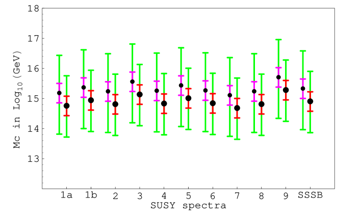
Figure 1: Compactification scale $M_{c}$ versus SUSY spectrum. For each SUSY spectrum, the bigger (smaller) circle on the right (left) shows the result in the HN (CPRT) approach. The shorter error bar represent the parametric error dominated by the experimental uncertainty on $\alpha_{3}(m_{Z})$, the wider bar includes the dominant source of error, the SU(5)-breaking brane terms.

Inputs to our computations are the experimental results in eq. (40) and the spectra of supersymmetric particles and extra Higgses given in section 2, tables 4 and 5. The brane contribution $\delta_{i}^{(b)}$ described in section 4.3 are taken as random variables in the interval of eq. (48), where they are generated with a flat distribution. Fig. 1 shows the compactification scale $M_{c}$ as a function of the spectrum of supersymmetric particles. The heavy threshold corrections are evaluated according to both the approaches HN (error bars on the right) and CPRT (error bars on the left) discussed in section 4.4. For each given SUSY spectrum there are two main sources of errors. One is the experimental error, approximately Gaussian, due to the uncertainties affecting the input parameters in eq. (40). This is largely dominated by the error on $\alpha_{3}(m_{Z})$ and is represented by the smallest error bar in the figures. The other one is theoretical, associated to the unknown SU(5)-violating kinetic terms at $y=\pi R/2$. This is a non-Gaussian error, since we have no reason to prefer any values of the parameters $\delta_{i}^{(b)}$ in the interval (48). The linear sum of these two errors is described by the largest error bar in our figures. The total error is therefore fully dominated by the theoretical one and it heavily affects the prediction of the compactification scale, that is predicted only up to an overall factor $10^{\pm 1}$. The prediction of $M_{c}$ also depends on the spectrum of SUSY particles at the TeV scale. The induced error on $M_{c}$ is however subdominant and the largest difference between the values of $M_{c}$ obtained by varying the SUSY spectrum is by a factor of 4, at most. Finally, also the treatment of the heavy thresholds gives rise to a theoretical uncertainty. The values of $M_{c}$ obtained by the HN procedure are systematically smaller, by approximately a factor 2$\div$ 3, with respect to those given by the CPRT approach.

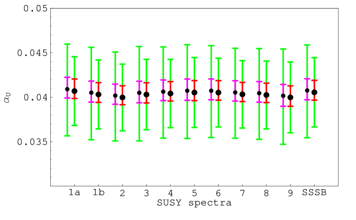
Figure 2: Gauge coupling $\alpha_{U}=g_{U}^{2}/(4\pi)$ at the compactification scale versus SUSY spectrum. Error bars as in fig. 1.

Despite the large overall uncertainty, from fig. 1 we see that on average the compactification scale $M_{c}$ is smaller than the unification scale of four-dimensional SUSY SU(5), $\approx 2\times 10^{16}$ GeV, by a factor of order 10. The effective gauge boson mass, $M_{X}=2M_{c}/\pi$, entering the dimension six operator of eqs. (27,35) is smaller than the corresponding mass in four-dimensional SUSY SU(5) by a factor $\approx 15$. This produces an average enhancement by a factor 5$\times 10^{4}$ in the proton decay rate. Moreover, the key point in the present analysis is that the theoretical uncertainties are completely dominated by the unknown SU(5) violating brane interactions and by the SUSY spectrum. Given the present knowledge, we cannot prefer any brane interactions or any SUSY spectrum among the various possibilities and the average prediction has not the meaning of the most probable one. From this viewpoint values of $M_{c}$ as small as $10^{14}$ GeV are equally probable than $M_{c}\approx 10^{15}$ GeV, and the enhancement of the proton decay rate can be as large as 5$\times 10^{8}$.

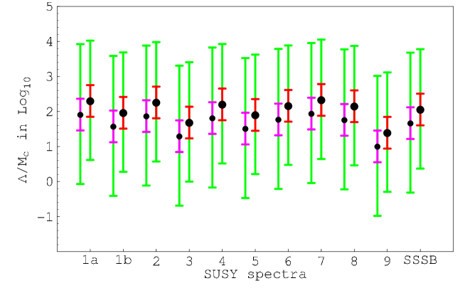
Figure 3: Ratio $\Lambda/M_{c}$ versus SUSY spectrum. Error bars as in fig. 1.

Such an enhancement is sufficient to overcome the huge suppression factor coming from flavor mixing in options I and II, which in the most favorable case, as we can see from table 6, is $|\lambda^{5}|^{2}\approx 3\times 10^{-7}$. From these considerations we can already conclude that the proton decay rate in the current model can be bigger by a factor $100$ compared to the the rate evaluated in four-dimensional SUSY SU(5) through dimension 6 operators. As we will see in the next section, we can obtain proton decay rates that are quite interesting for the next generation of experiments. Alternatively when considering option 0, where no flavour suppressions are present in the leading proton decay amplitudes, large values of $M_{c}$ such as $M_{c}\approx 10^{16}$ GeV allow to bring the proton lifetime above the experimental lower limit in eq. (1). Fig. 2 shows the predicted gauge coupling $\alpha_{U}$ at the compactification scale $M_{c}$. As we can see from eq. (35), this is an input to our computation and we evaluate it as the average among $\alpha_{i}(M_{c})$ $(i=1,2,3)$. We can see that $\alpha_{U}$ depends very mildly on the SUSY spectrum and on the treatment of heavy thresholds and is numerically close to 1/25, the value in ordinary four-dimensional SUSY SU(5). The error bars in fig. 2 have the same meaning as in fig. 1. When computing proton decay amplitudes what matters is the ratio $\alpha_{U}/M_{c}^{2}$, and we evaluate the errors on this quantity by fully accounting for correlations.

Finally, fig. 3 displays the dependence of the ratio $\Lambda/M_{c}$ on the SUSY spectrum, both for HN and CPRT cases. We can see that the average value of $\Lambda/M_{c}$ is about $100$, what needed for the dominance of the bulk symmetric SU(5) gauge coupling over the SU(5)-violating brane contribution in eq. (47). The ratio $\Lambda/M_{c}$ is also directly related to the parameter $\epsilon$ of eq. (17), which controls the hierarchies of Yukawa couplings. The range $\Lambda/M_{c}\approx 100$ is consistent, within the present approximations, with $\epsilon\approx\lambda^{2}$.

5 Proton lifetime

In order to calculate the proton lifetime, we have to translate the operators in (27,35,36) at quark level to those at hadron level using a perturbative chiral Lagrangian technique [33]. The aim is to evaluate the hadron matrix elements $\langle{\sl PS}\left|{\cal O}\right|p\rangle$, which describe the transition from the proton to a pseudoscalar meson via the three-quark operator ${\cal O}$.

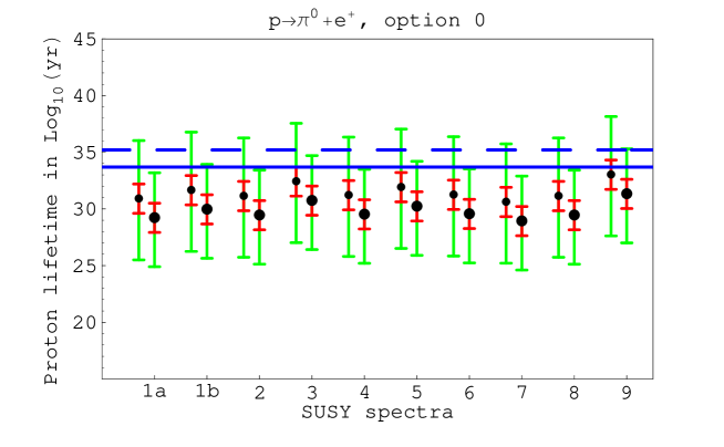
Figure 4: Inverse decay rate of $p\to\pi^{0}e^{+}$ versus the SUSY spectrum, in option 0. The solid line is the current experimental lower bound, from ref. [1], and the dashed line represents the aimed-for future sensitivity, from ref. [16]. Error bars as in fig. 1.

The various matrix elements are calculated from the basic element

$$\alpha\,P_{L}\,u_{p}=\epsilon_{\alpha\beta\gamma}\left\langle 0\left|\left(d_{R}^{\alpha}\,u_{R}^{\beta}\right)u_{L}^{\gamma}\right|p\right\rangle\,,$$ (60)

where $u_{p}$ denotes the proton spinor and $\alpha$ is evaluated by means of lattice QCD simulations. Here we will adopt [35]

$$\left|\alpha\right|=0.015~{}~{}{\rm GeV}^{3}~{}~{}~{}.$$ (61)

In option 0, the dominant decay rate is given by:

$$\Gamma(p\to e^{+}\pi^{0})=\frac{\displaystyle(m_{p}^{2}-m_{\pi^{0}}^{2})^{2}}{\displaystyle 64\pi m_{p}^{3}f_{\pi}^{2}}\,{\alpha^{2}}\,A^{2}_{S}A^{2}_{L}\;\frac{\displaystyle g_{U}^{4}}{\displaystyle M^{4}_{X}}\left(1+D+F\right)^{2}\,\left[\left(1+|V_{ud}|^{2}\right)+1\right]~{}~{}~{}.$$ (62)

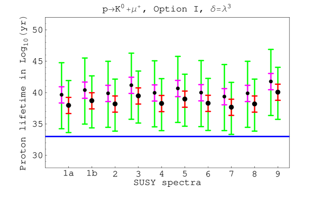
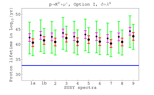
Figure 5: Inverse decay rate of $p\to K^{0}\mu^{+}$ versus the SUSY spectrum, in option I, for $\delta=\lambda^{3}$ (upper panel) and $\delta=\lambda^{4}$ (lower panel). The solid line is the current experimental lower bound, from ref. [1]. Error bars as in fig. 1.

Here $m_{p}$, $m_{\pi}$ denote the proton and pion masses respectively, and $f_{\pi}=130$ MeV is the pion decay constant; $D$ and $F$ are the symmetric and antisymmetric SU(3) reduced matrix elements for the axial-vector current and recent hyperon decays measurements [34] give $D=0.80$ and $F=0.46$. The effect of lepton masses is neglected. The short- and long-distance renormalization factors $A_{S}$, $A_{L}$ encode the evolution from the GUT scale to the SUSY-breaking scale and the evolution from the SUSY-breaking scale to 1 GeV [38]. We use:

$$A_{L}=\left(\frac{\alpha_{3}(\mu_{had})}{\alpha_{3}(m_{c})}\right)^{\frac{2}{9}}\left(\frac{\alpha_{3}(m_{c})}{\alpha_{3}(m_{b})}\right)^{\frac{6}{25}}\left(\frac{\alpha_{3}(m_{b})}{\alpha_{3}(m_{Z})}\right)^{\frac{6}{23}}\approx 1.43$$ (63)

with $\mu_{had}=1$ GeV and

$$A_{S}=\left(\frac{\alpha_{1}(m_{Z})}{\alpha_{U}}\right)^{\frac{23}{30b_{1}}}\left(\frac{\alpha_{2}(m_{Z})}{\alpha_{U}}\right)^{\frac{3}{2b_{2}}}\left(\frac{\alpha_{3}(m_{Z})}{\alpha_{U}}\right)^{\frac{4}{3b_{3}}}\approx 2.37$$ (64)

where the U(1) contribution is only approximate.

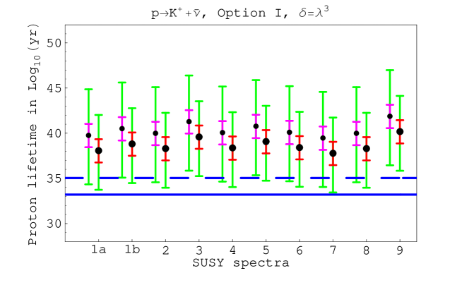
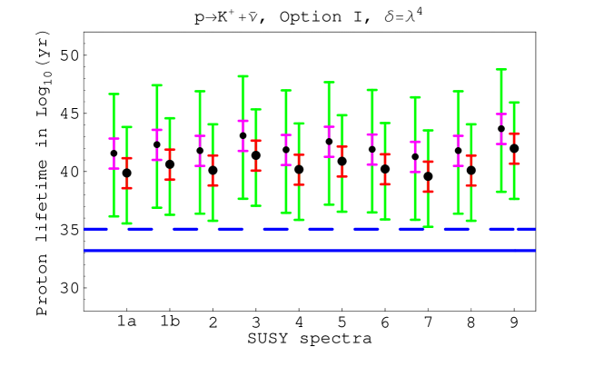
Figure 6: Inverse decay rate of $p\to K^{+}\nu$ (summed over all neutrino channels) versus the SUSY spectrum, in option I, for $\delta=\lambda^{3}$ (upper panel) and $\delta=\lambda^{4}$ (lower panel). The solid line is the current experimental lower bound, from ref. [1], and the dashed line represents the aimed-for future sensitivity, from ref. [16]. Error bars as in fig. 1.

In fig. 4 we see the predicted inverse decay rate as a function of the SUSY spectrum. A general comment, that applies to all the results concerning the rates in options 0, I and II, is that there is a huge theoretical uncertainty that spreads over many order of magnitudes. By far, the main source of this uncertainty is the compactification scale $M_{c}$, which is only know up to about two order of magnitudes, due to the unknown SU(5)-breaking brane contribution. Since the proton lifetime scales as $M_{c}^{4}$, this corresponds to an uncertainty of more than eight order of magnitudes on the inverse rates. In this enormous range the probability is however almost uniform. From fig. 4 we see that most of the parameter space of the model have already been excluded by the existing experimental bound. Though the model is not entirely ruled out and the allowed region in parameter space will be almost completely explored by the next generation of experiments.

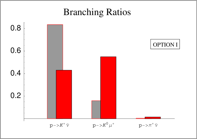
Figure 7: Branching ratios for option I. Dark-red (light-grey) histograms refer to $\delta=\lambda^{3}$ ($\delta=\lambda^{4}$).

The decay rates of option I and II for the different channels are given by:

$$\Gamma(p\to e_{j}^{+}\pi^{0}) = \frac{\displaystyle(m_{p}^{2}-m_{\pi^{0}}^{2})^{2}}{\displaystyle 64\pi m_{p}^{3}f_{\pi}^{2}}\,{\alpha^{2}}\,A^{2}_{S}A^{2}_{L}\;\frac{\displaystyle g_{U}^{4}}{\displaystyle M^{4}_{X}}\left(1+D+F\right)^{2}\,\left[|C^{1}_{j1}|^{2}+|C^{2}_{j1}|^{2}\right]$$

$$\Gamma(p\to e_{j}^{+}K^{0}) = \frac{\displaystyle(m_{p}^{2}-m_{K^{0}}^{2})^{2}}{\displaystyle 32\pi m_{p}^{3}f_{\pi}^{2}}\,{\alpha^{2}}\,A^{2}_{S}A^{2}_{L}\;\frac{\displaystyle g_{U}^{4}}{\displaystyle M^{4}_{X}}\left(1+\displaystyle\frac{m_{p}}{m_{B}}(D-F)\right)^{2}\,\left[|C^{1}_{j2}|^{2}+|C^{2}_{j2}|^{2}\right]$$

$$\Gamma(p\to\bar{\nu}_{j}\pi^{+}) = \displaystyle\frac{(m_{p}^{2}-m_{\pi^{\pm}}^{2})^{2}}{32\pi m_{p}^{3}f_{\pi}^{2}}\,{\alpha^{2}}\,A^{2}_{S}A^{2}_{L}\;\displaystyle\frac{g_{U}^{4}}{M^{4}_{X}}\left(1+D+F\right)^{2}\,|C^{3}_{11j}|^{2}$$

$$\Gamma(p\to\bar{\nu}_{j}K^{+}) = \displaystyle\frac{(m_{p}^{2}-m_{K^{\pm}}^{2})^{2}}{32\pi m_{p}^{3}f_{\pi}^{2}}\,{\alpha^{2}}A^{2}_{S}A^{2}_{L}\;\displaystyle\frac{g_{U}^{4}}{M^{4}_{X}}\times$$ (65)

$$\times\left|\displaystyle\frac{2}{3}\displaystyle\frac{m_{p}}{m_{B}}D~{}C^{3}_{12j}\!+\!\left(1+\displaystyle\frac{m_{p}}{3m_{B}}(D+3F)\right)C^{3}_{21j}\right|^{2}~{}~{}~{}.$$

Here $m_{K}$ denote the kaon mass and $m_{B}=1.15$ GeV is an average baryon mass according to contributions from diagrams with virtual $\Sigma$ and $\Lambda$. In our numerical estimates the interference in the expression of the rate for $K^{+}{\bar{\nu}}$ is constructive.

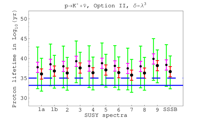
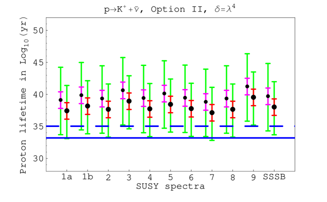
Figure 8: Inverse decay rate of $p\to K^{+}{\bar{\nu}}$ (summed over all neutrino channels) versus the SUSY spectrum, in option II, for $\delta=\lambda^{3}$ (upper panel) and $\delta=\lambda^{4}$ (lower panel). The solid line is the current experimental lower bound, from ref. [1], and the dashed line represents the aimed-for future sensitivity, from ref. [16]. Error bars as in fig. 1.

The dominant proton decay rates are shown in fig. (5,6) and (8-10). The results strongly depend on the location of $F_{1}$, either in the bulk (option I) or on the brane at $y=0$ (option II). As we can see from Table 4, if $F_{1}$ is a bulk field, then the dominant four-fermion operators are $uus\mu$ and $uds\nu_{\mu,\tau}$ and, consequently, the preferred proton decay channels are $K^{0}\mu^{+}$ and $K^{+}\nu$, whose rates are displayed in fig. (5,6). We see from fig. (5,6) that the possibilities of testing proton decay in option I are quite remote. If $\delta$, which parametrizes our ignorance about the mixing angles, is equal to $\lambda^{4}$, the inverse rates are always larger than 10³⁵ yr, too long to be observed in future planned facilities. When $\delta=\lambda^{3}$, only in some specific case the inverse rates can reach 10³⁴ yr, depending on the SUSY spectrum and on a favourable combination of the brane corrections $\delta_{i}^{(b)}$.

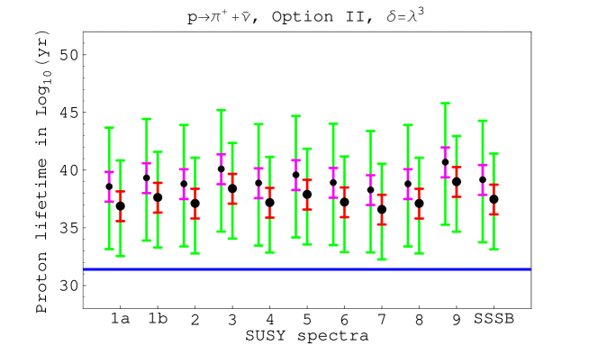
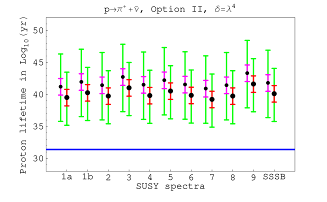
Figure 9: Inverse decay rate of $p\to\pi^{+}{\bar{\nu}}$ (summed over all neutrino channels) versus the SUSY spectrum, in option II, for $\delta=\lambda^{3}$ (upper panel) and $\delta=\lambda^{4}$ (lower panel). The solid line is the current experimental lower bound, from ref. [1]. Error bars as in fig. 1.

While the absolute rates are affected by a very large theoretical uncertainty, the predictions about the branching ratios are considerably more precise. The dependence on $M_{c}$ cancels out in the branching ratios and therefore the relative decay rates do not depend neither on the unknown SU(5)-breaking brane terms, nor on the SUSY spectrum. The uncertainty is dominated by the mixing matrices and is parametrized in our discussion by $\delta$, which we let vary between $\lambda^{3}$ and $\lambda^{4}$. In fig. 7 we see the BRs of the dominant channels in option I, $K^{+}{\bar{\nu}}$ and $K^{0}\mu^{+}$, which are comparable within the estimated uncertainty.

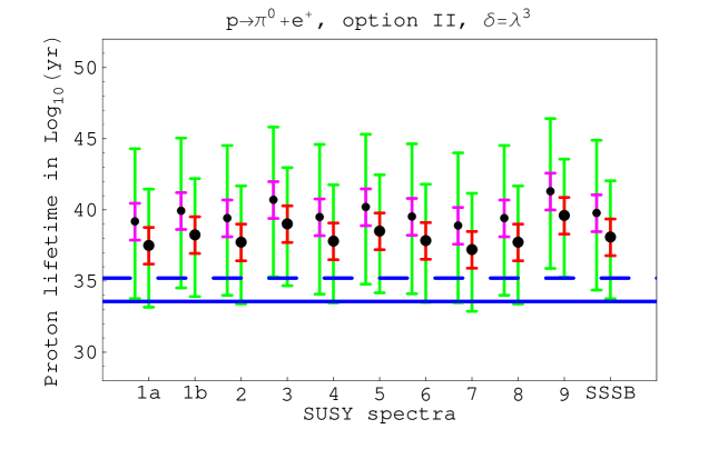
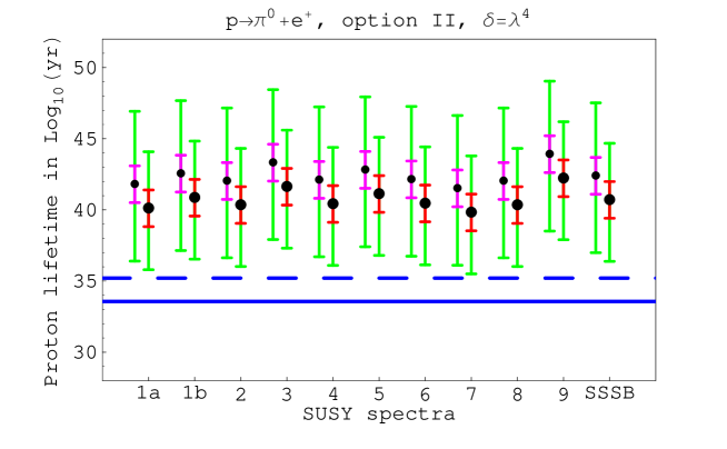
Figure 10: Inverse decay rate of $p\to\pi^{0}e^{+}$ (summed over all neutrino channels) versus the SUSY spectrum, in option II, for $\delta=\lambda^{3}$ (upper panel) and $\delta=\lambda^{4}$ (lower panel). The solid line is the current experimental lower bound, from ref. [1], and the dashed line represents the aimed-for future sensitivity, from ref. [16]. Error bars as in fig. 1.

Substantially different is the option II, where $F_{1}$ is a brane field like $F_{2,3}$. Here the preferred decay channel is $K^{+}{\bar{\nu}}$, as we can guess from Table 6, showing that this final state has the smallest flavour suppression. As we can see from fig. 8, a small portion of the parameter space of the model has already been excluded by the current experimental bound and, when $\delta=\lambda^{3}$, there will be good chances for the future facilities to discover proton decay in this channel, for almost all possible type of SUSY spectra considered in our analysis. Also if $\delta=\lambda^{4}$ and, consequently, the rates are more suppressed, there are several SUSY spectra which would allow a lifetime below $10^{35}$ yr, at least for some combination of the brane kinetic parameters $\delta_{i}^{(b)}$.

The rate for $\pi^{+}{\bar{\nu}}$ is down by approximately a factor $\lambda^{2}$, compared with the dominant one. Only for $\delta=\lambda^{3}$, for some specific SUSY spectra and in a favourable range of $\delta^{(b)}_{i}$, the predicted inverse rates are below $10^{34}$ yr, which would however represent an improvement over the current limit by more than two orders of magnitudes.

The prediction for the decay channels containing a charged lepton are similar to those for $\pi^{+}{\bar{\nu}}$, but the expected future experimental sensitivity is quite better, especially in the $\pi^{0}e^{+}$ mode, as shown in fig. 10. A modest portion of the parameter space, requiring $\delta$ close to $\lambda^{3}$, leads to inverse rates that are within the reach of future facilities.

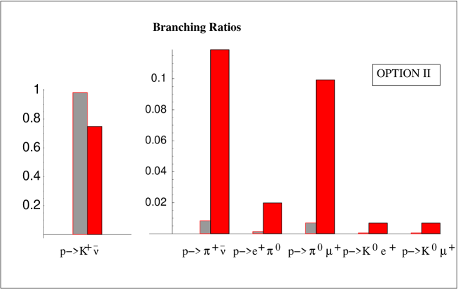
Figure 11: Branching ratios for option II. Dark-red (light-grey) histograms refer to $\delta=\lambda^{3}$ ($\delta=\lambda^{4}$).

The branching ratios for option II are displayed in fig. 11. We can see the dominance of $K^{+}{\bar{\nu}}$, followed by the $\pi^{+}{\bar{\nu}}$ and $\pi^{0}\mu^{+}$ channels. The other channels with a charged lepton, such as $\pi^{0}e^{+}$, $K^{0}e^{+}$ and $K^{0}\mu^{+}$ are comparable, but up to now future experimental prospects have been clearly worked out only for the $\pi^{0}e^{+}$ mode.

6 Conclusion

The decisive test of grand unification theories is proton decay. Minimal SUSY GUTs are strongly disfavoured today by the stringent experimental bounds on proton lifetime. Moreover such minimal realizations of the grand unification idea are also plagued by serious theoretical problems, first of all the doublet-triplet splitting problem, requiring a tuning by fourteen orders of magnitude. An elegant solution of the doublet-triplet splitting problem is offered by SUSY GUTs where the GUT symmetry is broken by the compactification of an extra dimension. There is a whole class of such GUTs where the leading baryon-violating operators arise from gauge vector boson exchange, have dimension six and scale as the inverse of the compactification mass $M_{c}$ squared.

We have evaluated $M_{c}$ form a next-to-leading analysis of gauge coupling unification including SUSY and GUT threshold corrections, two-loop running and SU(5)-breaking boundary terms. We have carefully estimated the uncertainties due to experimental errors and poor theoretical knowledge, such as the ignorance about the SUSY breaking spectrum and about the details of the SU(5)-breaking brane dynamics. In view of the existing intrinsic theoretical uncertainties we have found a wide range of acceptable values for $M_{c}$, going from approximately $10^{14}$ GeV to more than $10^{16}$ GeV.

The consequences on proton decay strongly depend on the features of the flavour sector, which can be considerably different from the standard, four-dimensional one. In the simplest case all matter fields have the same location in the extra space and proton decay proceeds mainly via the $\pi^{0}e^{+}$ channel, without any flavour suppression. Such a scenario is strongly disfavoured by now, since $M_{c}$ is on average much smaller than the four-dimensional unification scale $\approx 2\times 10^{16}$ GeV. However, due to the large uncertainties on $M_{c}$, it is not yet ruled out and future facilities can essentially complete the test of this model.

When matter fields have no identical location in the extra dimension, fermion mass hierarchies and mixing angles are more naturally described. In our analysis we have considered two options, corresponding to “semianarchy” (option I) and “anarchy” (option II) in the neutrino sector. In option I the suppression coming from flavour mixing is too strong and proton decay is almost beyond the possibilities of the next generation of experiments. In option II the flavour suppression of the $K^{+}{\bar{\nu}}$ channel can be compensated by the allowed smallness of $M_{c}$ resulting in a proton lifetime well within the reach of future facilities.

Acknowledgements We thank Luigi Pilo for useful discussions. This project is partially supported by the European Program MRTN-CT-2004-503369.

References

- [1] M. Shiozawa, in proceedings of the Workshop on “Neutrino Oscillations and their Origin” (NOON 2003), February 10-14 2003, Kanazawa, Japan.
- [2] H. Murayama and A. Pierce, Phys. Rev. D 65, 055009 (2002) [arXiv:hep-ph/0108104]. For a different viewpoint see: B. Bajc, P. Fileviez Perez and G. Senjanovic, Phys. Rev. D 66 (2002) 075005 [arXiv:hep-ph/0204311].
- [3] See, for instance, G. Altarelli, F. Feruglio and I. Masina, JHEP 0011 (2000) 040; I. Masina, Int. J. Mod. Phys. A 16 (2001) 5101. D. Emmanuel-Costa and S. Wiesenfeldt, Nucl. Phys. B 661 (2003) 62 [arXiv:hep-ph/0302272].
- [4] L. Randall and C. Csaki, presented at PASCOS / HOPKINS 1995 (Joint Meeting of the International Symposium on Particles, Strings and Cosmology, Baltimore, MD, March 22-25, 1995 and at the conference SUSY ’95, Palaiseau, France, May 15-19, 1995, arXiv:hep-ph/9508208.
- [5] E. Witten, Nucl. Phys. B 258 (1985) 75; A. E. Faraggi, Phys. Lett. B 520 (2001) 337 and references therein.
- [6] Y. Kawamura, Prog. Theor. Phys. 105 (2001) 999.
- [7] G. Altarelli and F. Feruglio, Phys. Lett. B 511 (2001) 257.
- [8] A. Hebecker and J. March-Russell, Nucl. Phys. B 613 (2001) 3.
- [9] L. J. Hall and Y. Nomura, Phys. Rev. D 64 (2001) 055003 [arXiv:hep-ph/0103125].
- [10] For a review see: J. Hisano, talk given at Workshop on Neutrinos Oscillations and Their Origin, Fijiyoshida, Japan, 11-13 Feb 2000. arXiv:hep-ph/0004266; see also J. Hisano, H. Murayama and T. Yanagida, Nucl. Phys. B 402 (1993) 46; D. Emmanuel-Costa and S. Wiesenfeldt, Nucl. Phys. B 661 (2003) 62; P. Fileviez Perez, Phys. Lett. B 595 (2004) 476; S. Wiesenfeldt, Mod. Phys. Lett. A 19 (2004) 2155.
- [11] Y. Nomura, Phys. Rev. D 65 (2002) 085036.
- [12] L. J. Hall and Y. Nomura, Phys. Rev. D 66 (2002) 075004.
- [13] R. Dermisek and A. Mafi, Phys. Rev. D 65 (2002) 055002; S. M. Barr and I. Dorsner, Phys. Rev. D 66 (2002) 065013; Q. Shafi and Z. Tavartkiladze, Phys. Rev. D 67 (2003) 075007; H. D. Kim and S. Raby, JHEP 0301 (2003) 056; B. Kyae, C. A. Lee and Q. Shafi, Nucl. Phys. B 683 (2004) 105; I. Dorsner, Phys. Rev. D 69 (2004) 056003; W. Buchmuller, L. Covi, D. Emmanuel-Costa and S. Wiesenfeldt, JHEP 0409 (2004) 004.
- [14] R. Contino, L. Pilo, R. Rattazzi and E. Trincherini, Nucl. Phys. B 622 (2002) 227.
- [15] A. Hebecker and J. March-Russell, Phys. Lett. B 539 (2002) 119.
- [16] C. K. Jung, arXiv:hep-ex/0005046; Y. Itow et al., arXiv:hep-ex/0106019; Y. Suzuki et al. [TITAND Working Group Collaboration], arXiv:hep-ex/0110005; A. Rubbia, arXiv:hep-ph/0407297.
- [17] See for instance, G. Altarelli and F. Feruglio, New J. Phys. 6 (2004) 106.
- [18] M. F. Sohnius, Phys. Rept. 128 (1985) 39.
- [19] H. Georgi and C. Jarlskog, Phys. Lett. B 86 (1979) 297; J. R. Ellis and M. K. Gaillard, Phys. Lett. B 88 (1979) 315.
- [20] H. Murayama, talk given at 22nd INS International Symposium on Physics with High Energy Colliders, Tokyo, Japan, 8-10 March 1994; arXiv:hep-ph/9410285; H. Murayama, talk at the 28th International Conference on High-energy Physics (ICHEP 96), Warsaw, Poland, 25-31 July 1996, arXiv:hep-ph/9610419.
- [21] A. Hebecker and J. March-Russell, Phys. Lett. B 541 (2002) 338.
- [22] J. Scherk and J. H. Schwarz, Phys. Lett. B 82 (1979) 60; J. Scherk and J. H. Schwarz, Nucl. Phys. B 153 (1979) 61.
- [23] P. Fayet, Phys. Lett. B 159 (1985) 121.
- [24] R. Barbieri, L. J. Hall and Y. Nomura, Phys. Rev. D 66 (2002) 045025; R. Barbieri, L. J. Hall and Y. Nomura, Nucl. Phys. B 624 (2002) 63.
- [25] L. J. Hall, H. Murayama and N. Weiner, Phys. Rev. Lett. 84 (2000) 2572; N. Haba and H. Murayama, Phys. Rev. D 63 (2001) 053010.
- [26] B. C. Allanach et al., in Proc. of the APS/DPF/DPB Summer Study on the Future of Particle Physics (Snowmass 2001) ed. N. Graf, Eur. Phys. J. C 25 (2002) 113.
- [27] See, for instance: G. Costa and F. Feruglio, Nuovo Cim. A 69 (1982) 195; G. Costa and F. Zwirner, Riv. Nuovo Cim. 9N3 (1986) 1.
- [28] S. Eidelman et al. [Particle Data Group Collaboration], Phys. Lett. B 592, 1 (2004).
- [29] D. R. T. Jones, Phys. Rev. D 25 (1982) 581; M. B. Einhorn and D. R. T. Jones, Nucl. Phys. B 196 (1982) 475.
- [30] See for instance: Y. Yamada, Z. Phys. C 60 (1993) 83.
- [31] H. Georgi, A. K. Grant and G. Hailu, Phys. Lett. B 506 (2001) 207 [arXiv:hep-ph/0012379].
- [32] P. Langacker and N. Polonsky, Phys. Rev. D 47 (1993) 4028 [arXiv:hep-ph/9210235].
- [33] M. Claudson, M. B. Wise and L. J. Hall, Nucl. Phys. B 195 (1982) 297.
- [34] N. Cabibbo, E. C. Swallow and R. Winston, Ann. Rev. Nucl. Part. Sci. 53, 39 (2003).
- [35] S. Aoki et al. [JLQCD Collaboration], Phys. Rev. D 62, 014506 (2000).
- [36] Y. Aoki [RBC Collaboration], Nucl. Phys. Proc. Suppl. 119 (2003) 380.
- [37] S. Raby, Rept. Prog. Phys. 67 (2004) 755 [arXiv:hep-ph/0401155].
- [38] L. E. Ibanez and C. Munoz, Nucl. Phys. B 245 (1984) 425; C. Munoz, Phys. Lett. B 177 (1986) 55.