CU-TP-1125
Extension of the JIMWLK equation in the low gluon density region

Abstract

It has recently been realized that the Balitsky-JIMWLK equations have serious shortcomings as equations to be used in small-$x$ evolution near the unitarity limit. A recent generalization of the Balitsky equations has been given which corrects these shortcomings. In this paper we present an equivalent discussion, but in terms of the JIMWLK equation where we show that a new (fourth order functional derivative) term should be included. We also present a stochastic version of the new equation which, however, has some unusual mathematical aspects which are not as yet well understood.

Keywords: JIMWLK equation, Balitsky equation, Kovchegov equation, BFKL equation, Langevin equation, Dipole Model, Fluctuations, Correlations

PACS numbers: 11.80.Fv, 11.80.La, 12.38.-t, 12.38.Bx

1 Introduction

The problem of high energy (small $x$) evolution near the unitarity limit [1] is one of the most important and widely studied problems in high energy QCD. A good understanding of this problem is necessary for understanding the energy dependence of the saturation momentum and other properties of the color glass condensate (CGC) [2]. This in turn is important for good understanding of such diverse quantities as the initial energy density produced just after a high energy heavy ion collision and the $Q^{2}$ and $x$-dependence of structure functions in deep inelastic scattering at small $x$ and at moderate values of $Q^{2}.$

The main equations that have been used to deal with high energy scattering near the unitarity limit are the Balitsky-JIMWLK equations [3, 4, 5, 6] and the Kovchegov equation [7]. The Balitsky equations are an infinite hierarchy of coupled equations expressing the energy dependence of the scattering of high energy quarks and gluons (represented by Wilson lines in the fundamental and adjoint representations, respectively) on a target. The Kovchegov equation results when the large-$N_{c}$ limit of the Balitsky hierarchy is taken along with dropping all correlations in the target. The Kovchegov equation is a (nonlinear) equation for a single function and, while no exact solution is known, the general properties of the solutions of this equation near the unitarity boundary are understood [8, 9, 10, 11, 12, 13, 14, 15, 16, 17, 18, 19, 20, 21, 22]. The JIMWLK equation is a functional Fokker-Planck equation which expresses small-x evolution of the target in a way which is exactly equivalent to the evolution of the scattering amplitudes given by the Balitsky equations. The JIMWLK equation is the basic equation for the CGC.

Geometric scaling [23] is a general property of solutions to the Kovchegov equation, and the exact (asymptotic) energy dependence of the saturation momentum [16, 17, 18] is also known for the Kovchegov equation. However, recently two of the present authors argued that while guaranteeing that overall scattering amplitudes satisfy unitarity limits the Kovchegov equation allows significant unitarity violation in intermediate stages of small-$x$ evolution [24]. These authors then proposed a simple prescription for suppressing the unitarity violations (a simple boundary limiting small size rare dipole fluctuations) without, however, realizing the generality of their prescription. Later, in Ref. [25], it was realized that the prescription was identical to a procedure used to study reaction-diffusion systems in statistical physics [26, 27], and that the prescription has a general validity for a certain class of observables such as the energy dependence of the saturation momentum. Again using the relationship between small-$x$ evolution and the time dependence of reaction-diffusion processes in statistical physics an asymptotic scaling law for the scattering amplitude, strongly violating geometric scaling was derived. This scaling differs from, but is related to, that found in Ref. [24] where fluctuations were not included in the purely mean field approach followed there.

Thus, the Kovchegov equation misses some essential aspects of high energy evolution near the unitarity boundary, although it may still be accurate for large nuclei or at intermediate energies. In this light the results of numerical simulations [28] comparing evolution using the Kovchegov equation with that using the Balitsky-JIMWLK equations come as a big surprise, because no essential differences were found. While this is partly due to the initial (Gaussian) distribution used in Ref. [28] the deeper understanding came from Iancu and Triantafyllopoulos [29] who noted that the Balitsky-JIMWLK equation also misses essential aspects of unitarity constraints. In the language of “Pomerons”, Balitsky-JIMWLK has Pomeron mergings but no Pomeron splittings. The authors of Ref. [29] then propose a generalization of the Balitsky equations which includes a stochastic part, thus allowing for Pomeron splittings, in addition to the usual Balitsky hierarchy. (In the context of Pomeron interactions this term, and its relationship to the dipole model, has been known for some time [31].) It is likely that the Balitsky hierarchy augmented by this new term contains the essential ingredients for small-$x$ evolution near the saturation boundary.

The discussion of Ref. [29] is given completely in terms of the Balitsky approach to high energy scattering. In this paper we give the corresponding (physically equivalent) discussion in the context of the JIMWLK approach. That is, we give a new equation, which includes the original contribution due to JIMWLK along with an extra term, the resulting equation having the form of a functional differential equation for the CGC weight function $W[\alpha]$. The JIMWLK equation, given below in Eq. (2.1), is a functional Fokker-Planck equation which has up to two derivatives of $W[\alpha]$ with respect to $\alpha$ but, in addition, has multiplicative powers of $\alpha$ such that there are always at least as many powers of $\alpha$ multliplying $W[\alpha]$ as there are $\alpha$-derivatives acting on $W[\alpha]$. The term having equal numbers of $\alpha$’s as derivatives of $\alpha$ generates the kernel for BFKL evolution while terms having extra powers of $\alpha$ correspond to “Pomeron mergings”. The absence of terms having more derivatives than factors of $\alpha$ is the absence of “Pomeron splittings.” The added new term has precisely four derivatives of $\alpha$ along with two factors of $\alpha$. The exact nature of this term is determined by requiring that it correspond to one parent dipole splitting into two daughter dipoles in the dipole model. If the parent dipole is part of a BFKL evolution, and if the two daughter dipoles undergo BFKL evolution as generated by the original terms in the JIMWLK equation, then our new term can be viewed as a single Pomeron splitting into two Pomerons. In Section 2 we carry out the construction of this splitting term with the resulting modified JIMWLK equation given in Eq. (2.24).

Our construction of this new term is carried out in the weak field limit where the dipole model [35, 37] is valid. We have no argument to the effect that it correctly represents Pomeron splittings in a strong field environment. On the other hand this new term is only important, as compared with the original terms in the JIMWLK equation, in the weak field limit so that we believe (2.24) represents the essential physics of BFKL evolution and unitarity constraints. That is, we believe that (2.24) is a good “effective” equation for small-$x$ evolution. If one wished to include higher order BFKL-kernel effects in the JIMWLK equation one could expect corrections to our new term also to be necessary, but in the context of evolution using the lowest order BFKL kernel, (2.24) should be sufficiently accurate. Iancu and Triantafyllopoulos [36] have observed that (2.24) is exactly equivalent to their new equation, and we also expect that it is equivalent to the procedure of unitarization developed some time ago by Salam [30], at least in the energy regime where that procedure is valid.

One of the very nice features of the JIMWLK equation is that it is possible to view it as a Langevin equation and hence use it as a basis for numerical simulations. Indeed, successful simulations have been performed by Rummukainen and Weigert [28]. This motivates trying to cast (2.24) in the form of a stochastic differential equation. In Section 3 this is done with, however, a few unusual aspects. In general a fourth order derivative will require a non-Gaussian noise, and this is illustrated by a simple example in Section 3.1. In Eq. (3.31) we give the rule for the evolution of $\alpha$ which, in a stochastic sense, is equivalent to (2.24). Eq. (3.31) involves three noise terms: $\zeta(\bm{z})$ is a fourth-order noise term, $\bar{\nu}^{a}(\bm{x},\bm{\omega})$ is a Gaussian noise term and $\xi(\bm{x},\bm{\omega})$ is a non-diagonal noise term whose correlator is given in (3.41). While we have been successful in casting our equation in the form of a stochastic differential equation the unusual form of the noise terms makes it unclear whether this form will be at all useful for numerical simulation. We do note, however, that the fourth-order noise terms have been discussed in the mathematical literature [33, 34], but we have not been able to find discussions of terms like our non-diagonal noise, and we are not certain that this term makes good mathematical sense.

2 Weak field extension of the JIMWLK equation

Iancu and Triantafyllopoulos [29] have recently recognized that the JIMWLK equation [4, 5, 6] – the basic equation of the Color Glass Condensate formalism – includes Pomeron mergings but not also Pomeron splittings which are important at low gluon densities (weak fields) in the wavefunction of a target. In this Section we extend the JIMWLK equation in the weak field regime by adding the Pomeron splittings.

2.1 JIMWLK equation

The JIMWLK equation [4, 5, 6] reads

$$\frac{\partial}{\partial Y}W_{Y}[\alpha]=\frac{1}{2}\int_{\bm{x},\bm{y}}\,\frac{\delta}{\delta\alpha_{Y}^{a}(\bm{x})}\,\eta^{ab}(\bm{x},\bm{y})\,\frac{\delta}{\delta\alpha_{Y}^{b}(\bm{y})}W_{Y}[\alpha]\ ,$$ (2.1)

where $Y=\ln 1/x$ is the rapidity of the small-$x$ gluons, $\int_{\bm{x}}\equiv\int d^{2}{\bm{x}}$ ($\bm{x}$, $\bm{y}$ denote transverse coordinates), $\alpha^{a}$ is the color gauge field radiated by the color sources in the target, and the functional $W_{Y}[\alpha]$ is the weight function for a given field configuration. The kernel $\eta^{ab}({\bm{x}},{\bm{y}})$ is a non–linear functional of $\alpha$,

$$\eta^{ab}(\bm{x},\bm{y})=\frac{1}{\pi}\int_{\bm{z}}\,{\cal K}({\bm{x},\bm{y},\bm{z}})\,(1-\tilde{V}^{\dagger}_{\bm{z}}\tilde{V}_{\bm{x}})^{fa}(1-\tilde{V}^{\dagger}_{\bm{z}}\tilde{V}_{\bm{y}})^{fb}\ ,$$ (2.2)

as it depends on the Wilson lines in the adjoint representation $\tilde{V}$ and $\tilde{V}^{\dagger}$,

$$\tilde{V}^{\dagger}_{\bm{x}}[\alpha]\,=\,{\rm P}\,{\rm exp}\left({\rm i}g\int dx^{-}\alpha^{a}(x^{-},{\bm{x}})T^{a}\right)\ ,$$ (2.3)

where $P$ denotes the path–ordering along the light-cone coordinate $x^{-}$ and

$${\cal K}({\bm{x},\bm{y},\bm{z}})=\frac{1}{(2\pi)^{2}}\,\frac{(\bm{x}-\bm{z})\cdot(\bm{y}-\bm{z})}{(\bm{x}-\bm{z})^{2}(\bm{z}-\bm{y})^{2}}\ .$$ (2.4)

The average of a generic operator $\cal{O}$ is defined as

$$\langle{\cal O}\rangle_{Y}\,=\,\int\,{\rm D}[\alpha]\,\,W_{Y}[\alpha]\,\,{\cal O}[\alpha]$$ (2.5)

and its evolution with respect to $Y$,

$$\frac{\partial\langle{\cal O}\rangle_{Y}}{\partial Y}\,=\,\left\langle{1\over 2}\int_{{\bm{x}},{\bm{y}}}\,{\delta\over{\delta\alpha^{a}({\bm{x}})}}\,\eta^{ab}({\bm{x}},{\bm{y}})\,{\delta\over{\delta\alpha^{b}({\bm{y}})}}\,{\cal O}[\alpha]\right\rangle_{Y}\ ,$$ (2.6)

follows by first using (2.1) and then integrating twice by parts in (2.5).

As an example, consider the scattering of a single dipole off a target. In the eikonal approximation, the T-matrix is given by

$$T({\bm{x}},{\bm{y}})\,=\,1-\frac{1}{N_{c}}\,{\rm tr}\Big{(}V^{\dagger}({\bm{x}})V({\bm{y}})\Big{)}\ ,$$ (2.7)

where $V^{\dagger}({\bm{x}})$ ($V({\bm{y}})$) is a Wilson line in the fundamental representation ($T^{a}\to t^{a}$ in (2.3)) which describes the scattering of the quark (antiquark) off the color field in the target, and the color trace divided by $N_{c}$ is the average over color. Inserting the above expression in Eq. (2.6), one obtains

$$\!\!\!\frac{\partial}{\partial Y}\langle T({\bm{x}},{\bm{y}})\rangle_{Y} = \frac{\alpha_{s}N_{c}}{2\pi^{2}}\int_{{\bm{z}}}\frac{(\bm{x}-\bm{y})^{2}}{(\bm{x}-\bm{z})^{2}(\bm{z}-\bm{y})^{2}}$$ (2.8)

$$\Big{\langle}-T({\bm{x}},{\bm{y}})+T({\bm{x}},{\bm{z}})+T({\bm{z}},{\bm{y}})-T({\bm{x}},{\bm{z}})T({\bm{z}},{\bm{y}})\Big{\rangle}_{Y}\ .$$

In this non-linear equation, the scattering of a single dipole $\langle T({\bm{x}},{\bm{y}})\rangle_{Y}$ on the l.h.s. is coupled to the scattering of two dipoles off the target $\langle T^{(2)}\rangle\equiv\langle T({\bm{x}},{\bm{z}})T({\bm{z}},{\bm{y}})\rangle_{Y}$ on the r.h.s., and, in general, the equation for $\langle T^{(N)}\rangle$ will involve also $\langle T^{(N+1)}\rangle$. So, Eq. (2.1) generates an infinite hierarchy of coupled non-linear equations. The same set of coupled equations has also been derived by Balitsky [3] in a frame where only the projectile evolves with increasing rapidity. Taking the large $N_{c}$ limit of the JIMWLK-Balitsky hierarchy (non-dipolar terms become neglegible) and dropping the correlations in the target ($\langle T({\bm{x}},{\bm{z}})T({\bm{z}},{\bm{y}})\rangle\to\langle T({\bm{x}},{\bm{z}})\rangle\,\langle T({\bm{z}},{\bm{y}})\rangle$), one obtains the Kovchegov equation [7] which is a closed equation for the $T$-matrix and, thus, much easier to handle than the coupled JIMWLK-Balitsky equations. Although no exact solution is known, the general properties of the solution to the Kovchegov equation are well understood [8, 9, 10, 11, 12, 13, 14, 15, 16, 17, 18, 19].

2.2 JIMWLK equation in the weak field limit

In the weak field limit ($\alpha\sim g\,\lower-1.93747pt\hbox{$<$}\kern-7.70004pt\lower 2.36806pt\hbox{$\sim$}\,1$), i.e., for low gluon density in the target, one can expand the kernel $\eta^{ab}$ in Eq. (2.2) in powers of $g$,

$$\eta^{ab}({\bm{x}},{\bm{y}})\,\simeq\,\frac{g^{2}\big{(}T^{c}T^{d}\big{)}_{ab}}{\pi}\int_{\bm{z}}\,{\cal K}({\bm{x},\bm{y},\bm{z}})\,\big{[}\alpha^{c}({\bm{x}})-\alpha^{c}({\bm{z}})\big{]}\big{[}\alpha^{d}({\bm{y}})-\alpha^{d}({\bm{z}})\big{]}$$ (2.9)

which when inserted in (2.6) yields

$$\frac{\partial\langle{\cal O}\rangle_{Y}}{\partial Y} = \frac{g^{2}\big{(}T^{c}T^{d}\big{)}_{ab}}{2\pi}$$

$$\times \!\!\!\!\int_{{\bm{x}},{\bm{y}},{\bm{z}}}\!\!\!\!\!{\cal K}({\bm{x},\bm{y},\bm{z}})\,\!\left\langle\!{\delta\over{\delta\alpha^{a}({\bm{x}})}}\,\big{[}\alpha^{c}({\bm{x}})\!-\!\alpha^{c}({\bm{z}})\big{]}\big{[}\alpha^{d}({\bm{y}})\!-\!\alpha^{d}({\bm{z}})\big{]}\,{\delta\over{\delta\alpha^{b}({\bm{y}})}}\,{\cal O}[\alpha]\right\rangle_{\!Y}\ ,$$

where

$$\alpha^{a}({\bm{x}})\,\equiv\,\int dx^{-}\,\alpha^{a}(x^{-},{\bm{x}})\ .$$ (2.11)

For the $T$-matrix (2.7) in the leading power in $g$,

$$T_{0}({\bm{x}},{\bm{y}})\,=\frac{g^{2}}{4N_{c}}\,\Big{(}\alpha^{a}({\bm{x}})-\alpha^{a}({\bm{y}})\Big{)}^{2}\,+\,{\cal O}(g^{3}),$$ (2.12)

equation (2.2) leads to the dipole version of BFKL equation [35]

$$\frac{\partial}{\partial Y}\langle T_{0}({\bm{x}},{\bm{y}})\rangle_{Y}=\frac{\alpha_{s}N_{c}}{2\pi^{2}}\int_{{\bm{z}}}\frac{(\bm{x}-\bm{y})^{2}}{(\bm{x}-\bm{z})^{2}(\bm{z}-\bm{y})^{2}}\Big{\langle}-T_{0}({\bm{x}},{\bm{y}})+T_{0}({\bm{x}},{\bm{z}})+T_{0}({\bm{z}},{\bm{y}})\Big{\rangle}_{Y}\ .$$ (2.13)

Note that in the weak field limit the JIMWLK equation (2.2) conserves the number of fields: two $\alpha$’s are created by $\alpha^{2}$ and two are destroyed by $(\delta/{\delta\alpha})^{2}$. The BFKL equation (2.13) is an example which shows that the evolution of a two-point correlation function (l.h.s) involves only two-point correlation functions (r.h.s). More generally, in the weak field limit, the evolution equation for an N-point correlation function involves only N-point correlation functions. In the language of perturbative QCD, the conservation of the number of fields corresponds to processes in which no Pomeron splitting or Pomeron merging in the t-channel is allowed.

The JIMWLK equation describes gluon (Pomeron) mergings in the hadron (nucleus) that are very important at high gluon densities (strong fields). This happens through the non-linearities in the JIMWLK equation: an N-point correlation function on the l.h.s. of (2.2) can involve in general all the M-point functions with M $\geq$ N on the r.h.s. once the higher orders in $\alpha$ ($\alpha^{n}$ with $n>2$) are taken into account in the expansion of $\eta^{ab}$ in (2.9). Gluon mergings reduce the number of fields in a correlation function. Fig. 1a shows the merging of $4$ gluons into $2$ gluons (or a $4$-point function reduces to a $2$-point function). A further BFKL evolution turns the $4$ to $2$ gluon merging into a $2$ to $1$ Pomeron merging via the triple pomeron vertex.

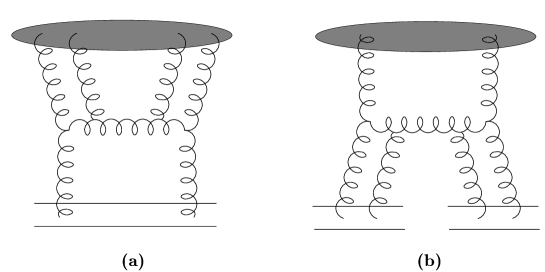
Figure 1: Target evolution: (a) gluon merging, (b) gluon splitting.

It has recently been recognized [29] that the JIMWLK equation does not provide gluon (Pomeron) splittings that turn out to be important for low gluon densities or weak fields in the target. This is because the JIMWLK equation (2.1) does not include higher order derivatives $(\delta^{n}/{\delta\alpha^{n}})$ with $n>2$ which in the weak field limit (where $\eta^{ab}\propto\alpha^{2}$) would generate gluon splittings. For instance, the JIMWLK equation does not include $\alpha^{2}(\delta^{4}/{\delta\alpha^{4}})$ which would generate a splitting of $2$ gluons into $4$ gluons (a $2$-point correlation function rises to a $4$-point correlation function) as shown in Fig. 1b. Thus, for low gluon densities in the target, there are no gluon number fluctations (Pomeron splittings) in the JIMWLK equation.

2.3 Extension of the JIMWLK equation in the weak field region based on the dipole model

In the next steps we will extend the JIMWLK equation (2.1) in the weak field regime by adding the gluon (Pomeron) splittings. We include the gluon number fluctuations in the JIMWLK equation based on the dipole model [35, 37] which is designed to properly describe the dilute region of a hadron wavefunction. The dipole model, on the other hand, has so far failed to accommodate gluon mergings, important at high gluon densities, which are a specialty of the JIMWLK equation.

To construct the weight function $W_{Y}[\alpha]$ of a target in the weak field limit based on the dipole model, we first need to know the weight function for a single dipole $W_{Y_{0}}[\alpha]$. The latter can be obtained by requiring that it gives the well-known result for dipole-dipole scattering in the $2$-gluon-exchange approximation when used to evaluate the averaging for the $T_{0}$-matrix (2.12) according to (2.5). The following weight function for a single dipole with coordinates ($\bm{x_{0}},\bm{y_{0}}$) [38]

$$W_{Y_{0}}[\alpha]\,=\,\left\{1+\frac{g^{2}}{4N_{c}}\int_{{\bm{u}},{\bm{v}}}\,{\cal G}({\bm{u}}|{\bm{x}}_{0},{\bm{y}}_{0}){\cal G}({\bm{v}}|{\bm{x}}_{0},{\bm{y}}_{0})\,\frac{\delta^{2}}{\delta\alpha^{a}({\bm{u}})\delta\alpha^{a}({\bm{v}})}\right\}\delta[\alpha]\ ,$$ (2.14)

gives the desired result for dipole-dipole scattering,

$$\langle T_{0}({\bm{x}},{\bm{y}})\rangle_{0}\, = \int\,{\rm D}[\alpha]\,\,W_{Y_{0}}[\alpha]\,T_{0}({\bm{x}},{\bm{y}})$$ (2.15)

$$= \frac{g^{4}N_{g}}{8N^{2}_{c}}\,\Big{(}{\cal G}({\bm{x}}|{\bm{x}}_{0},{\bm{y}}_{0})-{\cal G}({\bm{y}}|{\bm{x}}_{0},{\bm{y}}_{0})\Big{)}^{2}$$

$$= \frac{g^{4}N_{g}}{8N_{c}^{2}}\Big{[}\frac{1}{4\pi}\ln\frac{({\bm{x}}-{\bm{y}_{0}})^{2}({\bm{y}}-{\bm{x}_{0}})^{2}}{({\bm{x}}-{\bm{x}_{0}})^{2}({\bm{y}}-{\bm{y}_{0}})^{2}}\Big{]}^{2}\ ,$$

with the definitions

$${\cal G}({\bm{z}}|{\bm{x}}_{0},{\bm{y}}_{0})=\Delta({\bm{z}}-{\bm{x}_{0}})-\Delta({\bm{z}}-{\bm{y}_{0}})\ ,\quad\Delta(\bm{x})=\int\frac{d^{2}\bm{k}}{(2\pi)^{2}}\,\frac{e^{i\bm{k}\cdot\bm{x}}}{\bm{k}^{2}}=\frac{1}{4\pi}\ln\frac{1}{{\bm{x}}^{2}\mu^{2}}\ ,$$ (2.16)

and $N_{g}=N_{c}^{2}-1$. The infrared cutoff $\mu$ allows us to write down the propagator but it is harmless as it cancels in the difference in $\cal{G}$.

The weight function for N dipoles in the dipole model (DM) reads

$$W^{\mbox{\tiny DM}}_{Y}[\alpha]=\sum_{N=1}^{\infty}\int\!d\Gamma_{N}\,\,P_{N}(Y)\prod_{i=1}^{N}\!\bigg{\{}1+\frac{\lambda}{2}\!\int_{{\bm{u}},{\bm{v}}}\!\!{\cal G}_{i}({\bm{u}}){\cal G}_{i}({\bm{v}})\,\frac{\delta^{2}}{\delta\alpha^{a}({\bm{u}})\delta\alpha^{a}({\bm{v}})}\bigg{\}}\,\,\delta[\alpha]\ .$$ (2.17)

where

$${\cal G}_{i}({\bm{u}})\equiv{\cal G}({\bm{u}}|{\bm{x}_{i-1}},{\bm{x}_{i}})$$ (2.18)

with ${\bm{x}_{i-1}}$ and ${\bm{x}_{i}}$ the positions of the quark and the antiquark in the $i$th dipole. The shorthand notation $P_{N}(Y)$ denotes the probability to find a system of N dipoles with the transverse coordinates (${\bm{x}_{0}}$, ${\bm{x}_{1}}$), (${\bm{x}_{1}}$, ${\bm{x}_{2}}$), …(${\bm{x}_{N-1}}$, ${\bm{y}_{0}}$) via the evolution of an original dipole with coordinates (${\bm{x}_{0}}$, ${\bm{y}_{0}}$) up to rapidity $Y$. The phase space integration is $d\Gamma_{N}=d^{2}\bm{x}_{1}\,d^{2}\bm{x}_{2}...d^{2}\bm{x}_{N-1}$ and $\lambda=g^{2}/(2N_{c})$.

The evolution of the weight function (2.17) with increasing rapidity $Y$ is given by the following linear evolution equation

$$\frac{\partial}{\partial Y}W^{\mbox{\tiny DM}}_{Y}[\alpha]\!\! = \!\!\frac{\alpha_{s}N_{c}}{2\pi^{2}}\!\int_{\bm{x},\bm{y},\bm{z}}\frac{(\bm{x}-\bm{y})^{2}}{(\bm{x}-\bm{z})^{2}(\bm{z}-\bm{y})^{2}}$$ (2.19)

$$\times \!\!\!\!\!\Bigg{[}\,-\Big{(}1+\frac{\lambda}{2}\int_{{\bm{u}},{\bm{v}}}\,{\cal G}({\bm{u}}|{\bm{x}},{\bm{y}}){\cal G}({\bm{v}}|{\bm{x}},{\bm{y}})\,\frac{\delta^{2}}{\delta\alpha^{a}({\bm{u}})\delta\alpha^{a}({\bm{v}})}\Big{)}\Big{.}$$

$$+\Big{(}1+\frac{\lambda}{2}\int_{{\bm{u}_{1}},{\bm{v}_{1}}}\,{\cal G}({\bm{u}_{1}}|{\bm{x}},{\bm{z}}){\cal G}({\bm{v}_{1}}|{\bm{x}},{\bm{z}})\,\frac{\delta^{2}}{\delta\alpha^{a}({\bm{u_{1}}})\delta\alpha^{a}({\bm{v_{1}}})}\Big{)}\Big{.}$$

$$\times\Big{(}1+\frac{\lambda}{2}\int_{{\bm{u}_{2}},{\bm{v}_{2}}}\,{\cal G}({\bm{u}_{2}}|{\bm{z}},{\bm{y}}){\cal G}({\bm{v}_{2}}|{\bm{z}},{\bm{y}})\,\frac{\delta^{2}}{\delta\alpha^{b}({\bm{u_{2}}})\delta\alpha^{b}({\bm{v_{2}}})}\Big{)}\Bigg{]}$$

$$\times\Big{(}\frac{1}{-2\lambda N_{g}}\Big{)}\,\nabla^{2}_{\bm{x}}\,\nabla^{2}_{\bm{y}}\,\alpha^{c}(\bm{x})\,\alpha^{c}(\bm{y})\,W^{\mbox{\tiny DM}}_{Y}[\alpha]\ .$$

This equation is a sum of two terms: a virtual term (loss term) and a real term (gain term) as we know them from the dipole model. The term $\nabla^{2}_{\bm{x}}\,\nabla^{2}_{\bm{y}}\,\alpha(\bm{x})\,\alpha(\bm{x})$ plays the role of an annihilation operator for a dipole while $(1+\lambda/2\int{\cal G}^{2}(\partial/\partial\alpha)^{2})$ corresponds to a creation operator for a dipole. In the virtual term a dipole is destroyed and its coordinates are transfered to the new one which is created. In the real term a dipole is converted into two new ones with the right coordinates and splitting factors.

To explicitly show the annihilation and creation of dipoles, consider the evaluation of (2.19) with an arbitrary function ${\cal O}[\alpha]$

$${\cal I}\equiv\int\,{\rm D}[\alpha]\,\,\left(\frac{\partial W^{\mbox{\tiny DM}}_{Y}[\alpha]}{\partial Y}\right)\,\,{\cal O}[\alpha]\ .$$ (2.20)

$\cal{I}$ will be zero unless one takes the functional derivatives from one of the dipoles in (2.17) and integrates them by parts in (2.20) on the $\alpha(\bm{x})\,\alpha(\bm{y})$ term. Using

$$\!\!\!\!\frac{\lambda}{2}\,\int_{{\bm{u}},{\bm{v}}}\!{\cal G}_{i}({\bm{u}}){\cal G}_{i}({\bm{v}})\,\frac{\delta^{2}}{\delta\alpha^{a}({\bm{u}})\delta\alpha^{a}({\bm{v}})}\,\nabla^{2}_{\bm{x}}\,\nabla^{2}_{\bm{y}}\,\alpha^{c}(\bm{x})\,\alpha^{c}(\bm{y})$$

$$\hskip 28.45274pt=\lambda N_{g}\left[\delta(\bm{x}-\bm{x_{i-1}})-\delta(\bm{x}-\bm{x_{i}})\right]\left[\delta(\bm{y}-\bm{x_{i-1}})-\delta(\bm{y}-\bm{x_{i}})\right]$$

one gets

$$\frac{\partial}{\partial Y}W^{\mbox{\tiny DM}}_{Y}[\alpha]\!\! = \!\!\frac{\alpha_{s}N_{c}}{2\pi^{2}}\,\sum_{i=1}^{N}\,\int_{\bm{x_{i-1}},\bm{x_{i}},\bm{z}}\frac{(\bm{x_{i}}-\bm{x_{i-1}})^{2}}{(\bm{x_{i-1}}-\bm{z})^{2}(\bm{z}-\bm{x_{i}})^{2}}$$

$$\times \!\!\!\!\!\Bigg{[}\,-\Big{(}1+\frac{\lambda}{2}\int_{{\bm{u}},{\bm{v}}}\,{\cal G}({\bm{u}}|{\bm{x_{i-1}}},{\bm{x_{i}}}){\cal G}({\bm{v}}|{\bm{x_{i-1}}},{\bm{x_{i}}})\,\frac{\delta^{2}}{\delta\alpha^{a}({\bm{u}})\delta\alpha^{a}({\bm{v}})}\Big{)}\Bigg{.}$$

$$+\Big{(}1+\frac{\lambda}{2}\int_{{\bm{u}_{1}},{\bm{v}_{1}}}\,{\cal G}({\bm{u}_{1}}|{\bm{x_{i-1}}},{\bm{z}}){\cal G}({\bm{v}_{1}}|{\bm{x_{i-1}}},{\bm{z}})\,\frac{\delta^{2}}{\delta\alpha^{a}({\bm{u_{1}}})\delta\alpha^{a}({\bm{v_{1}}})}\Big{)}\Big{.}$$

$$\times\Big{(}1+\frac{\lambda}{2}\int_{{\bm{u}_{2}},{\bm{v}_{2}}}\,{\cal G}({\bm{u}_{2}}|{\bm{z}},{\bm{x_{i}}}){\cal G}({\bm{v}_{2}}|{\bm{z}},{\bm{x_{i}}})\,\frac{\delta^{2}}{\delta\alpha^{b}({\bm{u_{2}}})\delta\alpha^{b}({\bm{v_{2}}})}\Big{)}\Bigg{]}$$

$$\times\sum_{N=1}^{\infty}\int\!d\Gamma_{N}^{\prime}\,\,P_{N}(Y)\prod_{{j=1}\atop{j\neq i}}^{N}\!\bigg{\{}1+\frac{\lambda}{2}\!\int_{{\bm{u}},{\bm{v}}}\!\!{\cal G}_{j}({\bm{u}}){\cal G}_{j}({\bm{v}})\,\frac{\delta^{2}}{\delta\alpha^{c}({\bm{u}})\delta\alpha^{c}({\bm{v}})}\bigg{\}}\,\,\delta[\alpha],$$

where $d\Gamma_{N}^{\prime}$ means that the $\bm{x_{i-1}}$ and $\bm{x_{i}}$ coordinate integrations are missing. By comparing this equation with (2.19), we now explicitly see that the evolution is the same one known from the dipole model: When increasing the rapidity in one step, the $N$-dipole system either survives as it is (virtual term) or it evolves by splitting one of the dipoles into two new dipoles (real term). In the latter, the kernel (times $\alpha_{s}N_{c}/(2\pi^{2})$) in the first line in (2.3) is the right factor to turn $P_{N}$ into $P_{N+1}$ while the product of the terms in the third and fourth line are what is needed for converting the original $\bm{i}$th dipole into two new dipoles ($\bm{x_{i-1}}$, $\bm{z}$) and ($\bm{z}$, $\bm{x_{i}}$).

One can rewrite the evolution equation (2.3) also in the form

$$\frac{\partial W^{\mbox{\tiny DM}}_{Y}[\alpha]}{\partial Y}=\sum_{N=1}^{\infty}\int\!d\Gamma_{N}\,\,\frac{\partial P_{N}(Y)}{\partial Y}\prod_{i=1}^{N}\!\bigg{\{}1+\frac{\lambda}{2}\!\int_{{\bm{u}},{\bm{v}}}\!\!{\cal G}_{i}({\bm{u}}){\cal G}_{i}({\bm{v}})\,\frac{\delta^{2}}{\delta\alpha^{a}({\bm{u}})\delta\alpha^{a}({\bm{v}})}\bigg{\}}\,\,\delta[\alpha]\ ,\\$$ (2.22)

which is consistent with Eq. (2.17). The identification of (2.22) with (2.3) gives the evolution equation for the probabilities (see [38])

$$\frac{\partial P_{N}(Y|\bm{x_{1}},...,\bm{x_{N-1}})}{\partial Y}=\!\!\! - \!\!\!\frac{\alpha_{s}N_{c}}{2\pi^{2}}\bigg{[}\sum_{i=1}^{N}\int_{\bm{z}}\frac{(\bm{x}_{i-1}-\bm{x}_{i})^{2}}{(\bm{x}_{i-1}-\bm{z})^{2}(\bm{x}_{i}-\bm{z})^{2}}\bigg{]}P_{N}(Y|\bm{x_{1}},...,\bm{x_{N-1}})$$ (2.23)

$$+\,\frac{\alpha_{s}N_{c}}{2\pi^{2}}\sum_{i=1}^{N-1}\frac{(\bm{x}_{i-1}-\bm{x}_{i+1})^{2}}{(\bm{x}_{i-1}-\bm{{x}_{i}})^{2}(\bm{x}_{i+1}-\bm{{x}_{i}})^{2}}\,\,P_{N-1}(Y|\bm{x_{1}},...,\bm{x_{i-1}},\bm{x_{i+1}}...,\bm{x_{N-1}})\ ,$$

where $P_{N}(Y|\bm{x_{1}},...,\bm{x_{N-1}})$ denotes the probability for $N$-dipoles with coordinates (${\bm{x}_{0}}$, ${\bm{x}_{1}}$), (${\bm{x}_{1}}$, ${\bm{x}_{2}}$), …(${\bm{x}_{N-1}}$, ${\bm{y}_{0}}$) generated by the evolution of an original dipole with coordinates ($\bm{x_{0}}$, $\bm{y_{0}}$). The first term is a loss term which describes the emission of one gluon from the original $N$-dipole system while the second term is a gain term which describes the formation of the $N$-dipole system via the splitting of one dipole in an original $(N-1)$-dipole system. It is the loss term which takes into account gluon (Pomeron) splittings missed in the JIMWLK equation [29, 30]. Furthermore, it is easy to show that the probability is conserved by (2.23) [38]: $\sum_{i=1}^{N}\int d{\Gamma}_{N}P_{N}(Y)=1$.

Let’s now compare the evolution equation (2.19) which follows from the dipole model with the JIMWLK equation in the weak field limit. The three $\cal{G}\cal{G}$ terms in (2.19) correspond to ordinary BFKL evolution while the $\cal{G}\cal{G}\cal{G}\cal{G}$ term allows Pomeron splitting. Since the ordinary BFKL terms were already properly included in the JIMWLK equation, only the final, $\cal{G}\cal{G}\cal{G}\cal{G}$, term has to be added to the JIMWLK equation. Thus, the main result of this work reads

$$\!\!\!\!\!\!\!\!\frac{\partial}{\partial Y}W_{Y}[\alpha]=\Bigg{(}\frac{1}{2}\int_{\bm{x},\bm{y}}\,\frac{\delta}{\delta\alpha_{Y}^{a}(\bm{x})}\,\eta^{ab}(\bm{x},\bm{y})\,\frac{\delta}{\delta\alpha_{Y}^{b}(\bm{y})}$$

$$\!\!\!\!\!\!\!-\,\frac{N_{c}^{2}}{8\pi^{3}N_{g}}\!\int_{\textstyle{{\bm{x},\bm{y},\bm{z}}\atop{\bm{u_{1}},\bm{v_{1}},\bm{u_{2}},\bm{v_{2}}}}}\!\!\!\!\!\left(\frac{\lambda}{2}\right)^{2}\!\!\!\frac{(\bm{x}-\bm{y})^{2}}{(\bm{x}-\bm{z})^{2}(\bm{z}-\bm{y})^{2}}\,{\cal G}({\bm{u}_{1}}|{\bm{x}},{\bm{z}}){\cal G}({\bm{v}_{1}}|{\bm{x}},{\bm{z}}){\cal G}({\bm{u}_{2}}|{\bm{z}},{\bm{y}}){\cal G}({\bm{v}_{2}}|{\bm{z}},{\bm{y}})$$

$$\!\!\!\!\!\!\times\,\frac{\delta}{\delta\alpha^{a}({\bm{u_{1}}})}\,\frac{\delta}{\delta\alpha^{a}({\bm{v_{1}}})}\,\frac{\delta}{\delta\alpha^{b}({\bm{u_{2}}})}\,\frac{\delta}{\delta\alpha^{b}({\bm{v_{2}}})}\,\nabla^{2}_{\bm{x}}\,\nabla^{2}_{\bm{y}}\,\alpha^{c}(\bm{x})\,\alpha^{c}(\bm{y})\Bigg{)}\,W_{Y}[\alpha]\ .$$ (2.24)

Our derivation of the Pomeron splitting term, $\cal{G}\cal{G}\cal{G}\cal{G}$ term in (2.24), is done in the weak field limit. Therefore we cannot say that it also correctly describes Pomeron splittings in the presence of strong fields ($\alpha\sim 1/g$), or high gluon densities, in the target. However, since the Pomeron splitting term is important only in the weak field limit ($\alpha\sim g$) as compared with the original JIMWLK term, we believe that (2.24) is a good “effective” equation for small-$x$ evolution which includes the essential physics of BFKL evolution and unitarity constraints. Our Pomeron splitting term should be accurate enough as long as the evolution involves only the lowest order BFKL-kernel. Corrections to the new term are expected if higher order BFKL-kernel effects are included in the original JIMWLK term.

The extended JIMWLK equation (2.24) includes Pomeron mergings and Pomeron splittings and, thus, through iterations, Pomeron loops. This equation is equivalent to the new equation derived by Iancu and Triantafyllopoulos [36], and it should also be equivalent to the procedure of unitarization developed by Salam [30] in which the gluon number fluctuations are properly treated. We expect that the solution to Eq. (2.24) will confirm the results of the recent works [24, 25]. In these works it has been shown that due to the fluctuations the rate of growth of the saturation momentum (the “saturation exponent”) considerably decreases and the geometric scaling [23] property is strongly violated as compared to the numerical results of the Balitsky-JIMWLK equation and the Kovchegov equation given in [28]. The latter equations miss the fluctuations or the Pomeron loops.

Below we write the extended JIMWLK equation (2.24) in a form which is more appropriate for its stochastic interpretation given in the next Section [6, 32]:

$$\!\!\!\!\!\!\!\!\frac{\partial}{\partial Y}W_{Y}[\alpha]=\Bigg{(}-\frac{\delta}{\delta\alpha^{a}({\bm{x}})}\,\sigma^{a}({\bm{x}})+\frac{1}{2}\int_{\bm{x},\bm{y}}\,\frac{\delta^{2}}{\delta\alpha_{Y}^{a}(\bm{x})\delta\alpha_{Y}^{b}(\bm{y})}\,\eta^{ab}(\bm{x},\bm{y})$$

$$\!\!\!\!\!\!\!-\,\frac{N_{c}^{2}}{8\pi^{3}N_{g}}\!\int_{\textstyle{{\bm{x},\bm{y},\bm{z}}\atop{\bm{u_{1}},\bm{v_{1}},\bm{u_{2}},\bm{v_{2}}}}}\!\!\!\!\!\left(\frac{\lambda}{2}\right)^{2}\!\!\!\frac{(\bm{x}-\bm{y})^{2}}{(\bm{x}-\bm{z})^{2}(\bm{z}-\bm{y})^{2}}\,{\cal G}({\bm{u}_{1}}|{\bm{x}},{\bm{z}}){\cal G}({\bm{v}_{1}}|{\bm{x}},{\bm{z}}){\cal G}({\bm{u}_{2}}|{\bm{z}},{\bm{y}}){\cal G}({\bm{v}_{2}}|{\bm{z}},{\bm{y}})$$

$$\!\!\!\!\!\!\times\,\frac{\delta}{\delta\alpha^{a}({\bm{u_{1}}})}\,\frac{\delta}{\delta\alpha^{a}({\bm{v_{1}}})}\,\frac{\delta}{\delta\alpha^{b}({\bm{u_{2}}})}\,\frac{\delta}{\delta\alpha^{b}({\bm{v_{2}}})}\,\nabla^{2}_{\bm{x}}\,\nabla^{2}_{\bm{y}}\,\alpha^{c}(\bm{x})\,\alpha^{c}(\bm{y})\Bigg{)}\,W_{Y}[\alpha]\ ,$$ (2.25)

with

$$\sigma^{a}({\bm{x}})=\frac{1}{2}\int_{\bm{y}}\frac{\delta}{\delta\alpha^{b}({\bm{y}})}\eta^{ab}({\bm{x}},{\bm{y}})\ .$$ (2.26)

The original JIMWLK equation (first two terms in (2.25)) is the familiar functional Fokker-Planck equation [6, 32] which describes a diffusion process with $\sigma^{a}({\bm{x}})$ giving the drift term and $\eta^{a,b}({\bm{x}},{\bm{y}})$ the diffusion coefficient. A Langevin equation for the fields $\alpha(x)$ can be written down which is equivalent to the original JIMWLK equation [32]. The extended JIMLWK equation (2.25) is more complicated as it contains also the fourth order derivatives with respect to $\alpha$ (Pomeron splitting) in addition to the familiar Fokker-Planck equation. In the next Section we show how to obtain a stochastic differential equation also for the extended JIMWLK equation. The hope hereby is that one may use the stochastic differential equation for numerical simulations of (2.25) as done for the original JIMWLK equation in [28].

3 Interpretation of the evolution equation in terms of noise

A functional equation like the JIMWLK equation although written in an elegant compact form (not so compact after adding our extension for a dilute color medium) is hard to use in actual computations. But this obstacle can be surmounted via the observation that JIMWLK resembles very much a diffusion equation [32] which describes the time evolution of molecules undergoing Brownian motion. The latter has the interpretation of particles subjected to random acceleration in the medium, in other words a Langevin interpretation of the motion of the particles. In the case of JIMWLK, it is the light-cone gauge fields $\alpha^{a}({\bm{x}})$ that acquire a Gaussian random noise. In the previous section it was shown that in the case of a weak field a fourth order differential term was required to fully take into account all the important contributions at the leading log level. Unfortunately the extended JIMWLK equation ceases to be a functional diffusion equation of the Fokker-Planck type and the Langevin description is ruined. In this section we aim to restore the stochastic description even though the Langevin interpretation is mostly irreversibly lost. This requires a multi-random noise description involving both Gaussian white noise as well as other higher order noise. We will first show the basics of how a purely fourth order differential equation can arise out of a non-Gaussian random noise introduced at the fundamental level of the equation of motion. Then progressing in increasing complexity a Langevin term will be added which is well known to be responsible for the second order diffusion equation. Thus one will eventually have a multi-noise stochastic differential equation as the equation of motion from which the extended JIMWLK equation can be recovered.

3.1 Illustration with some simple toy models

To demonstrate the essentials of how to arrive at a fourth order differential equation using random noise, we consider a system of particles whose motions, similar to molecules undergoing Brownian motion, are Markov in nature. That means what happens to the system of particle next in time depends only on the present state and not in any way on the history of this system of particles. As we will see, this crucial condition simplifies the probabilistic description tremendously when the probability density distribution at one time can be related to a previous time in a relatively simple manner. Thus it is tempting to try to stay within the framework of Brownian motion, however we shall see that this is not really possible.

3.1.1 A 1+1 dimensional system

To start off, let’s consider the probability distribution, $P(x,t)$, of our system of particles which is a function of position $x$ and time $t$. The motion of the particles is taken to obey the stochastic equation

$$\dot{x}(t)=\sigma(x)+(\gamma(x))^{1/4}\,\zeta(t)$$ (3.1)

where $\sigma(x)$ is the deterministic mean drift of the particles, $\gamma(x)$ is some function of $x$, and $\zeta(t)$ is a non-Gaussian random noise which has a normalized distribution (suppressing for the moment the $t$ dependence)

$${\mbox{\rm d}}{\cal P}_{{}_{\mbox{\scriptsize NG}}}(\zeta)=f_{{}_{\mbox{\scriptsize NG}}}(\zeta)\,{\mbox{\rm d}}\zeta\;,$$ (3.2)

so that

$$\int f_{{}_{\mbox{\scriptsize NG}}}(\zeta)\,{\mbox{\rm d}}\zeta=1\;.$$ (3.3)

Using the notation

$$\langle{\cal O}(\zeta)\rangle_{{}_{\mbox{\scriptsize NG}}}=\int{\cal O}(\zeta)f_{{}_{\mbox{\scriptsize NG}}}(\zeta)\,{\mbox{\rm d}}\zeta$$ (3.4)

to denote an average over the distribution $f_{{}_{\mbox{\scriptsize NG}}}(\zeta)$, the random noise obeys

$$\langle\zeta\rangle_{{}_{\mbox{\scriptsize NG}}}=\langle\zeta^{2}\rangle_{{}_{\mbox{\scriptsize NG}}}=\langle\zeta^{3}\rangle_{{}_{\mbox{\scriptsize NG}}}=0\;,$$ (3.5)

and is only nonzero first in the four $\zeta$ correlator

$$\langle\zeta^{4}\rangle_{{}_{\mbox{\scriptsize NG}}}=c_{{}_{\mbox{\scriptsize NG}}}$$ (3.6)

where $c_{{}_{\mbox{\scriptsize NG}}}$ is a number. This is the reason that $\zeta$ is referred to as a fourth order noise in the literature [33, 34]. In that sense the usual Gaussian noise is second order noise. Note that the distribution $f_{{}_{\mbox{\scriptsize NG}}}(\zeta)$ cannot be written down simply as a function of some compact form but must be expressed in terms of a Fourier transform. The explicit expression $f_{{}_{\mbox{\scriptsize NG}}}(\zeta)$ serves little purpose in our discussion here and will not be written down. What is important here are the correlators given above, the first nonvanishing correlator is the one with four $\zeta$’s whereas it is the two noise correlator in the case of the Gaussian noise that is the first nonvanishing one.

Given that the particle motion is Markov in nature, the probability distribution of the particles $P(x,t)$ must depend on $P(x^{\prime},t^{\prime})$ where the particles currently at $x$ arrived there by previously first reaching $x^{\prime}$ at an earlier time $t^{\prime}$. Bayes’ theorem states the conditional probability $P(A|B)$ relating the probability $P(A)$ of an event A happening given that another related event B has already happened with probability $P(B)$ must satisfy

$$P(A)=P(A|B)P(B)\;.$$ (3.7)

It follows that

$$P(x,t)=\int{\mbox{\rm d}}x^{\prime}P(x,t|x^{\prime},t^{\prime})P(x^{\prime},t^{\prime})\;.$$ (3.8)

For a small time increment $\delta t$ so that $t^{\prime}=t-\delta t$, the particle motion, from Eq. (3.1), changes by

$$\delta x(t)=x-x^{\prime}=\Big{[}\sigma(x^{\prime})+(\gamma(x^{\prime}))^{1/4}\,\zeta(t)\Big{]}\,\delta t\;.$$ (3.9)

Since $\zeta$ is a stochastic variable given the present position $x$, the previous $x^{\prime}$ is therefore non-deterministic but has a distribution. The conditional probability $P(x,t|x^{\prime},t^{\prime})$ is therefore given by

$$P(x,t|x^{\prime},t^{\prime})=\int{\mbox{\rm d}}{\cal P}_{{}_{\mbox{\scriptsize NG}}}(\zeta(t))\,\delta(x-x^{\prime}-[\sigma(x^{\prime})+(\gamma(x^{\prime}))^{1/4}\,\zeta(t)]\,\delta t)\;.$$ (3.10)

In the limit that $\delta t$ becomes very small, one can Taylor expand the $\delta$-function in powers of $\delta t$, but one has to keep terms up to the fourth power of $\delta t$ if they are accompanied by a corresponding power of $\zeta$

$$P(x,t|x^{\prime},t^{\prime})\simeq\int{\mbox{\rm d}}{\cal P}_{{}_{\mbox{\scriptsize NG}}}(\zeta(t))\!\!\!\! \!\!\!\!\Big{\{}\delta(x-x^{\prime})-\delta^{\prime}(x-x^{\prime})\Big{[}\sigma(x^{\prime})+(\gamma(x^{\prime}))^{1/4}\,\zeta(t)\Big{]}\,\delta t$$ (3.11)

$$+\frac{1}{2}\delta^{{}^{\prime\prime}}(x-x^{\prime})\Big{[}\sigma(x^{\prime})+(\gamma(x^{\prime}))^{1/4}\,\zeta(t)\Big{]}^{2}\,\delta t^{2}$$

$$-\frac{1}{3!}\delta^{{}^{\prime\prime\prime}}(x-x^{\prime})\Big{[}\sigma(x^{\prime})+(\gamma(x^{\prime}))^{1/4}\,\zeta(t)\Big{]}^{3}\,\delta t^{3}$$

$$+\frac{1}{4!}\delta^{{}^{\prime\prime\prime\prime}}(x-x^{\prime})\Big{[}\sigma(x^{\prime})+(\gamma(x^{\prime}))^{1/4}\,\zeta(t)\Big{]}^{4}\,\delta t^{4}$$

$$+\dots\Big{\}}\;.$$

Here we have written $\partial\delta(x-x^{\prime})/\partial x=\delta^{\prime}(x-x^{\prime})=-\partial\delta(x-x^{\prime})/\partial x^{\prime}$. In view of Eq. (3.5) and Eq. (3.6), the above expansion can be simplified to

$$\!P(x,t|x^{\prime},t^{\prime})\simeq\delta(x-x^{\prime})-\delta^{\prime}(x-x^{\prime})\,\sigma(x^{\prime})\,\delta t+\frac{1}{4!}c_{{}_{\mbox{\scriptsize NG}}}\delta^{{}^{\prime\prime\prime\prime}}(x-x^{\prime})\,\gamma(x^{\prime})\,\delta t^{4}+\dots\;.$$ (3.12)

Substituting this into Eq. (3.8) and expanding

$$P(x^{\prime},t-\delta t)\simeq P(x^{\prime},t)-\frac{\partial P(x^{\prime},t)}{\partial t}\delta t+\dots$$ (3.13)

as well, after some rearrangements and using $c_{{}_{\mbox{\scriptsize NG}}}=-1/\delta t^{3}$, one finally has

$$\frac{\partial P(x,t)}{\partial t}=-\frac{\partial\,\sigma(x)P(x,t)}{\partial x}-\frac{1}{4!}\frac{\partial^{4}\,\gamma(x)P(x,t)}{\partial x^{4}}\;.$$ (3.14)

The negative sign of $c_{{}_{\mbox{\scriptsize NG}}}$ is necessary for the stable evolution of $P(x,t)$. One can see that fourth order diffusion can be associated with a fourth order noise much in the same way that the Gaussian white noise gives rise to the second order diffusion equation.

3.1.2 A 2+1 dimensional system

Let’s now consider a system that has an evolution equation for its probability distribution that bears more resemblance to the equation in Sec 2. Since the CGC evolution equation exists both in the functional space which is really infinite dimensional as well as the color space of QCD, we extend our system to two spatial dimensions. This should suffice to demonstrate the main features of the noise interpretation of our equation. In addition JIMWLK is basically a diffusion equation so there must be a stochastic term for the white noise as well. We will let the motion of the particles in this system obey

$$\dot{x}^{i}(t)=\sigma^{i}({\bm{x}})+\epsilon^{ij}({\bm{x}})\,\nu^{j}(t)+(\gamma({\bm{x}}))^{1/4}\,G_{ab}({\bm{x}})\bar{\nu}^{i}_{a}(t)\,\zeta_{b}(t)\;.$$ (3.15)

$\sigma^{i}(x)$ is the deterministic drift as before, which is followed by the term of the Gaussian white noise $\nu^{j}$ with the tensor coefficient function $\epsilon^{ij}({\bm{x}})$. $\nu^{i}$ has the usual normalized Gaussian distribution

$$d{\cal P}_{{}_{\mbox{\scriptsize G}}}(\nu)=f_{{}_{\mbox{\scriptsize G}}}(\nu)\,{\mbox{\rm d}}^{2}\nu\;,$$ (3.16)

$$\int f_{{}_{\mbox{\scriptsize G}}}(\nu)\,{\mbox{\rm d}}^{2}\nu=1\;.$$ (3.17)

and expectation

$$\langle{\cal O}(\nu)\rangle_{{}_{\mbox{\scriptsize G}}}=\int{\cal O}(\nu)f_{{}_{\mbox{\scriptsize G}}}(\nu)\,{\mbox{\rm d}}^{2}\nu\;.$$ (3.18)

The white noise $\nu^{i}(t)$ of course has all the usual properties

$$\langle\nu^{i}\rangle_{{}_{\mbox{\scriptsize G}}}=0$$ (3.19)

and

$$\langle\nu^{i}\nu^{j}\rangle_{{}_{\mbox{\scriptsize G}}}=c_{{}_{\mbox{\scriptsize G}}}\,\delta^{ij}\;.$$ (3.20)

The last term of Eq. (3.15) is the fourth order noise term but now with more complicated functions as its coefficient as well as a set of secondary random Gaussian distributed variables $\bar{\nu}^{i}_{a}$. The last have the normalized distribution

$${\mbox{\rm d}}\bar{P}_{{}_{\mbox{\scriptsize G}}}(\bar{\nu}_{a})=\bar{f}_{{}_{\mbox{\scriptsize G}}}(\bar{\nu}_{a})\,{\mbox{\rm d}}^{2}\bar{\nu}_{a}\;,$$ (3.21)

which gives

$$\langle\bar{\nu}^{i}_{a}\bar{\nu}^{j}_{b}\rangle_{{}_{\mbox{\scriptsize G}}}=\delta^{ij}\,\delta_{ab}\;.$$ (3.22)

The form of Eq. (3.15) is peculiar but is necessary to arrive at the extended evolution equation. Proceeding in a similar fashion to the previous subsection with a small time increment

$$\delta x^{i}(t)=x^{i}-x^{\prime i}=\Big{[}\sigma^{i}({\bm{x}}^{\prime})+\epsilon^{ij}({\bm{x}}^{\prime})\,\nu^{j}(t)+(\gamma({\bm{x}}^{\prime}))^{1/4}\,G_{ab}({\bm{x}}^{\prime})\bar{\nu}^{i}_{a}(t)\,\zeta_{b}(t)\Big{]}\delta t\;.$$ (3.23)

Bayes’ theorem gives us

$$P({\bm{x}},t)=\int{\mbox{\rm d}}^{2}{\bm{x}}^{\prime}P({\bm{x}},t|{\bm{x}}^{\prime}t^{\prime})P({\bm{x}}^{\prime},t^{\prime})\;,$$ (3.24)

with the conditional probability

$$P({\bm{x}},t|{\bm{x}}^{\prime}t^{\prime})\! = \!\int{\mbox{\rm d}}{\cal P}_{{}_{\mbox{\scriptsize G}}}(\nu)\,\prod_{a}{\mbox{\rm d}}\bar{\cal P}_{{}_{\mbox{\scriptsize G}}}(\bar{\nu}_{a})\,{\mbox{\rm d}}{\cal P}_{{}_{\mbox{\scriptsize NG}}}(\zeta)$$

$$\!\!\times\delta^{2}({\bm{x}}-{\bm{x}}^{\prime}-[\sigma^{i}({\bm{x}}^{\prime})+\epsilon^{ij}({\bm{x}}^{\prime})\,\nu^{j}(t)+(\gamma({\bm{x}}^{\prime}))^{1/4}\,G_{ab}({\bm{x}}^{\prime})\bar{\nu}^{i}_{a}(t)\,\zeta_{b}(t)]\delta t)$$

which once again can be expanded or one can equally apply Ito’s lemma. Bearing in mind all the vanishing correlators of the different noise, we have

$$P({\bm{x}},t|{\bm{x}}^{\prime}t^{\prime})=\!\!\!\! \!\!\!\!\int{\mbox{\rm d}}{\cal P}_{{}_{\mbox{\scriptsize G}}}(\nu)\,\prod_{a}{\mbox{\rm d}}\bar{\cal P}_{{}_{\mbox{\scriptsize G}}}(\bar{\nu}_{a})\,{\mbox{\rm d}}{\cal P}_{{}_{\mbox{\scriptsize NG}}}(\zeta)$$ (3.26)

$$\Big{\{}\delta^{2}({\bm{x}}-{\bm{x}}^{\prime})-\sigma^{i}({\bm{x}}^{\prime})\,\partial^{i}\delta^{2}({\bm{x}}-{\bm{x}}^{\prime})\delta t$$

$$+\frac{1}{2!}\epsilon^{im}({\bm{x}}^{\prime})\epsilon^{jn}({\bm{x}}^{\prime})\nu^{m}(t)\nu^{n}(t)\partial^{i}\partial^{j}\delta^{2}({\bm{x}}-{\bm{x}}^{\prime})\,\delta t^{2}$$

$$+\frac{1}{4!}\gamma({\bm{x}}^{\prime})\,G_{ab}({\bm{x}}^{\prime})G_{cd}({\bm{x}}^{\prime})G_{ef}({\bm{x}}^{\prime})G_{gh}({\bm{x}}^{\prime})\,\bar{\nu}^{i}_{a}(t)\bar{\nu}^{j}_{c}(t)\bar{\nu}^{k}_{e}(t)\bar{\nu}^{l}_{g}(t)\,$$

$$\;\;\times\zeta_{b}(t)\zeta_{d}(t)\zeta_{f}(t)\zeta_{h}(t)\,\partial^{i}\partial^{j}\partial^{k}\partial^{l}\delta^{2}({\bm{x}}-{\bm{x}}^{\prime})\,\,\delta t^{4}$$

$$+\dots\Big{\}}\;.$$

After making use of Eq. (3.20), Eq. (3.22), the modified version of Eq. (3.6),

$$\langle\zeta_{b}(t)\zeta_{d}(t)\zeta_{f}(t)\zeta_{h}(t)\rangle=c_{{}_{\mbox{\scriptsize NG}}}\delta_{bd}\,\delta_{df}\,\delta_{fh}\ ,$$ (3.27)

the notation from [32],

$$\eta^{ij}({\bm{x}})=\epsilon^{ik}({\bm{x}})\,\epsilon^{jk}({\bm{x}})\ ,$$ (3.28)

and not forgetting that the correlator of four Gaussian noise isn’t zero but can be separated into a sum of products of two two Gaussian noise correlators,

$$\langle\bar{\nu}^{i}_{a}\bar{\nu}^{j}_{c}\bar{\nu}^{k}_{e}\bar{\nu}^{l}_{g}\rangle_{{}_{\mbox{\scriptsize G}}}=\langle\bar{\nu}^{i}_{a}\bar{\nu}^{j}_{c}\rangle_{{}_{\mbox{\scriptsize G}}}\langle\bar{\nu}^{k}_{e}\bar{\nu}^{l}_{g}\rangle_{{}_{\mbox{\scriptsize G}}}\\ +\langle\bar{\nu}^{i}_{a}\bar{\nu}^{k}_{e}\rangle_{{}_{\mbox{\scriptsize G}}}\langle\bar{\nu}^{j}_{c}\bar{\nu}^{l}_{g}\rangle_{{}_{\mbox{\scriptsize G}}}\\ +\langle\bar{\nu}^{i}_{a}\bar{\nu}^{l}_{g}\rangle_{{}_{\mbox{\scriptsize G}}}\langle\bar{\nu}^{j}_{c}\bar{\nu}^{k}_{e}\rangle_{{}_{\mbox{\scriptsize G}}}\ ,$$

one gets

$$\frac{\partial P({\bm{x}},t)}{\partial t}=-\frac{\partial\sigma^{i}({\bm{x}})P({\bm{x}},t)}{\partial x^{i}}+\frac{1}{2!}\frac{\partial^{2}\eta^{ij}({\bm{x}})P({\bm{x}},t)}{\partial x^{i}\partial x^{j}}-\frac{1}{4!}\frac{\partial^{4}\Delta^{ijkl}({\bm{x}})P({\bm{x}},t)}{\partial x^{i}\partial x^{j}\partial x^{k}\partial x^{l}}\;,$$ (3.29)

where $c_{{}_{\mbox{\scriptsize G}}}=1/\delta t$ has been taken  and

$$\Delta^{ijkl}({\bm{x}})\!\!\! = \!\!\!\gamma({\bm{x}})\,G_{ab}({\bm{x}})G_{cb}({\bm{x}})G_{eb}({\bm{x}})G_{gb}({\bm{x}})$$ (3.30)

$$\times\Big{(}\delta_{ac}\delta_{eg}\delta^{ij}\delta^{kl}+\delta_{ae}\delta_{cg}\delta^{ik}\delta^{jl}+\delta_{ag}\delta_{ce}\delta^{il}\delta^{jk}\Big{)}\;.$$

This equation has all the basic features of Eq. (2.25) but some fine tuning is still required. This is the subject of the next subsection.

3.2 Noise interpretation of the extended JIMWLK equation

Back to our present problem, the JIMWLK equation is a functional equation of the integrated light-cone gauge field $\alpha^{a}$ and the evolution is in rapidity $Y$ rather than in time so one has to replace $t$ by $Y$ everywhere. In analogy to the equation for $\dot{x}^{i}$ before, we write the stochastic equation

$$\frac{\partial}{\partial Y}\alpha^{a}({\bm{u}})=\sigma^{a}({\bm{u}})+\int_{\bm{z}}\epsilon^{ab,i}({\bm{u}},{\bm{z}})\nu^{b,i}({\bm{z}})+\int_{{\bm{x}},{\bm{w}},{\bm{z}}}\rho({\bm{u}},{\bm{x}},{\bm{w}},{\bm{z}})\bar{\nu}^{a}({\bm{x}},{\bm{w}})\zeta({\bm{z}})\sqrt{\xi({\bm{x}},{\bm{w}})}$$ (3.31)

where borrowing again from the notation of [32]  the first stochastic term with the Gaussian noise $\nu^{b,i}$ has the tensor coefficient function

$$\epsilon^{ab,i}({\bm{u}},{\bm{z}})=\frac{1}{\sqrt{4\pi^{3}}}\frac{({\bm{u}}-{\bm{z}})^{i}}{({\bm{u}}-{\bm{z}})^{2}}(1-V^{\dagger}_{\bm{u}}V_{\bm{z}})^{ab}$$ (3.32)

and the product

$$\eta^{ab}({\bm{u}},{\bm{v}})=\int_{\bm{z}}\epsilon^{ac,i}({\bm{u}},{\bm{z}})\epsilon^{bc,i}({\bm{v}},{\bm{z}})$$ (3.33)

from which the first deterministic term $\sigma^{a}({\bm{u}})$ can be expressed as

$$\sigma^{a}({\bm{u}})=\frac{1}{2}\int_{\bm{v}}\frac{\delta}{\delta\alpha^{b}({\bm{v}})}\eta^{ab}({\bm{u}},{\bm{v}})\;.$$ (3.34)

The last multi-noise stochastic term on the right hand side of Eq. (3.31) has a second but different Gaussian noise $\bar{\nu}^{a}({\bm{x}},{\bm{w}})$, the fourth order noise $\zeta({\bm{z}})$ and a new noise $\xi({\bm{x}},{\bm{w}})$ which we call a non-diagonal noise for reason which will become clear later with a normalized distribution

$$\int{\mbox{\rm d}}{\cal P}_{{}_{\mbox{\scriptsize ND}}}(\xi)=1\;.$$ (3.35)

The coefficient function of this last term is

$$\rho({\bm{u}},{\bm{x}},{\bm{w}},{\bm{z}})=\sqrt{\frac{\lambda N_{c}}{({\bm{x}}-{\bm{z}})^{2}}}\bigg{\{}\frac{4!({\bm{x}}-{\bm{w}})^{2}(\nabla^{2}_{\bm{x}}\nabla^{2}_{\bm{w}}\alpha^{c}({\bm{x}})\alpha^{c}({\bm{w}}))}{3\cdot 2^{5}\pi^{3}N_{g}}\bigg{\}}^{1/4}{\cal G}({\bm{u}}|{\bm{x}},{\bm{z}})\;.$$ (3.36)

Here we consider an evolution of the probability density $W_{Y}[\alpha]$ of the color fields of the CGC by a small increment from $Y^{\prime}=Y-\delta Y$ to $Y$

$$W_{Y}[\alpha]=\int{\mbox{\rm D}}[\alpha^{\prime}]\,P_{Y|Y^{\prime}}[\alpha|\alpha^{\prime}]\,W_{Y^{\prime}}[\alpha^{\prime}]$$ (3.37)

during which the fields $\alpha^{a}$ make the change

$$\delta\alpha^{a}=\alpha^{a}-\alpha^{{}^{\prime}a}=\delta Y\,\frac{\partial}{\partial Y}\alpha^{a}\;.$$ (3.38)

The conditional probability here is

$$P_{Y|Y^{\prime}}[\alpha|\alpha^{\prime}] = \int\prod_{a,i}[{\mbox{\rm D}}{\cal P}_{{}_{\mbox{\scriptsize G}}}(\nu^{a,i})]\prod_{b}[{\mbox{\rm D}}\bar{\cal P}_{{}_{\mbox{\scriptsize G}}}(\bar{\nu}^{b})][{\mbox{\rm D}}{\cal P}_{{}_{\mbox{\scriptsize NG}}}(\zeta)][{\mbox{\rm D}}{\cal P}_{{}_{\mbox{\scriptsize ND}}}(\xi)]$$ (3.39)

$$\;\;\times\delta^{N_{g}}(\alpha-\alpha^{\prime}-\delta Y\,\partial\alpha/\partial Y)\;.$$

This is written slightly differently than before because of the functional aspect of Eq. (3.37). The measures of the noise $[{\mbox{\rm D}}{\cal P}]$ here are now path integrals for the same reason, and $\partial\alpha/\partial Y$ is given by Eq. (3.31). Either using Ito’s lemma or expanding the delta function in terms of $\delta Y$, $W_{Y^{\prime}}[\alpha^{\prime}]$ in terms of $\delta Y$ as before and substituting in Eq. (3.37), the original JIMWLK equation is straightforwardly recovered by following the steps in the previous subsection [32]. The term that is less trivial is the four derivative Pomeron splitting term which comes essentially from the last term of Eq. (3.31) raised to the fourth power or the collection of all the apparent $\delta Y^{4}$ terms in the expansion of the delta function in Eq. (3.39). At this order of the expansion, each functional derivative $\delta/\delta\alpha^{a}$ is accompanied by $\zeta({\bm{z}})$ whose correlator ensures that there is only one $z$ coordinate via

$$\langle\zeta({\bm{z}})\zeta({\bm{z}}^{\prime})\zeta({\bm{z}}^{\prime\prime})\zeta({\bm{z}}^{\prime\prime\prime})\rangle_{{}_{\mbox{\scriptsize NG}}}=c_{{}_{\mbox{\scriptsize NG}}}\delta^{2}({\bm{z}}-{\bm{z}}^{\prime})\delta^{2}({\bm{z}}^{\prime}-{\bm{z}}^{\prime\prime})\delta^{2}({\bm{z}}^{\prime\prime}-{\bm{z}}^{\prime\prime\prime})\ ,$$ (3.40)

where here $c_{{}_{\mbox{\scriptsize NG}}}=-1/\delta Y^{3}$. This is the case as seen in Eq. (2.25), the new term has four ${\cal G}$ functions sharing the same ${\bm{z}}$ as one endpoint to a pair of dipoles. This is the result of a one-step evolution from a single parent dipole. Each of the four ${\cal G}({\bm{u}}|{\bm{x}},{\bm{z}})$’s coming from the fourth order expansion of Eq. (3.39) is a contribution to the field $\alpha({\bm{u}})$ from a dipole with endpoints ${\bm{x}}$ and ${\bm{z}}$. Or equivalently each dipole interacts with the target through two gluon exchanges, each of which is represented by a ${\cal G}({\bm{u}}|{\bm{x}},{\bm{z}})$ therefore the four ${\cal G}({\bm{u}}|{\bm{x}},{\bm{z}})$’s must come in two pairs with each pair sharing the same endpoints. The presence of the second Gaussian noise $\bar{\nu}^{a}({\bm{x}},{\bm{w}})$ correlator $\langle\bar{\nu}^{a}({\bm{x}}_{1},{\bm{w}}_{1})\bar{\nu}^{b}({\bm{x}}_{2},{\bm{w}}_{2})\bar{\nu}^{c}({\bm{x}}_{3},{\bm{w}}_{3})\bar{\nu}^{d}({\bm{x}}_{4},{\bm{w}}_{4})\rangle_{{}_{\mbox{\scriptsize G}}}$, which can be rewritten in a similar fashion to Eq. (3.1.2), guarantees that this is the case. These mostly ensure that one inevitably arrives at Eq. (2.25) except the numerator of the BFKL kernel, which is $({\bm{x}}-{\bm{y}})^{2}$. Naively one is required to put the quartic root of this expression in the stochastic equation for $\alpha^{a}$ in Eq. (3.31) which is impossible since only one of ${\bm{x}}$ and ${\bm{y}}$ can appear in the expression. The other comes into Eq. (2.25) via the $\delta Y$ expansion and the $\bar{\nu}$ correlator discussed above. Thus to ensure that the appearance of the correct BFKL kernel, we gave the factor ${\{({\bm{x}}-{\bm{w}})^{2}\}}^{1/4}$ to Eq. (3.31), introduced the very unconventional non-diagonal noise $\sqrt{\xi({\bm{x}},{\bm{w}})}$ and required the latter to satisfy the correlation

$$\langle\xi({\bm{x}},{\bm{w}})\xi({\bm{y}},{\bm{w}}^{\prime})\rangle_{{}_{\mbox{\scriptsize ND}}}=\delta^{2}({\bm{x}}-{\bm{w}}^{\prime})\delta^{2}({\bm{y}}-{\bm{w}})\;.$$ (3.41)

One should note the unusual pairing of the arguments of the $\delta$-functions. This is the reason for its nomenclature. Here two sets of coordinate pair have already been identified as ${\bm{x}},{\bm{w}}$ and ${\bm{y}},{\bm{w}}^{\prime}$ thanks to the $\bar{\nu}^{a}$ correlators so the square root has been removed. This correlation is somewhat counterintuitive because one encounters much more frequently the normal Gaussian noise, whose correlator is

$$\langle\xi({\bm{x}},{\bm{w}})\xi({\bm{y}},{\bm{w}}^{\prime})\rangle_{{}_{\mbox{\scriptsize G}}}=\delta^{2}({\bm{x}}-{\bm{y}})\delta^{2}({\bm{w}}-{\bm{w}}^{\prime})\;.$$ (3.42)

As it is the non-diagonal correlator requires that a squared quantity to be zero

$$\langle\xi({\bm{x}},{\bm{w}})^{2}\rangle_{{}_{\mbox{\scriptsize ND}}}=0\;.$$ (3.43)

This demands a lot on the distribution itself. The only constraint on $\xi({\bm{x}},{\bm{w}})$ here is Eq. (3.35) and Eq. (3.41). Note that although $\sqrt{\xi({\bm{x}},{\bm{w}})}$ appears in the stochastic equation Eq. (3.31), one does not encounter correlators such as

$$\langle\sqrt{\xi({\bm{x}},{\bm{w}})}\rangle_{{}_{\mbox{\scriptsize ND}}}\;\;,\;\;\langle\sqrt{\xi({\bm{x}},{\bm{w}})\xi({\bm{x}}^{\prime},{\bm{w}}^{\prime})}\rangle_{{}_{\mbox{\scriptsize ND}}}$$

etc because of the presence of $\bar{\nu}^{a}({\bm{x}},{\bm{w}})$ and $\zeta({\bm{x}})$. Such correlators are not only unpleasant but also not very meaningful. We are unable to find such an unusual correlator in the mathematics literature but if the stochastic interpretation of Eq. (2.25) is to be preserved, one would have to require such a correlator to exist. Note that the vanishing of the average over a squared quantity similar to Eq. (3.43) is also required of the fourth order noise $\zeta$ for which one knows that a distribution does exist. Providing one accepts that a distribution for $\xi$ might probably exist then with all the ingredients in place Eq. (2.25) can be reproduced from the multi-noise stochastic equation Eq. (3.31) by going through the steps as shown in this section. So once again although the extended JIMWLK equation for a dilute color dipole medium appears to be more complicated with a fourth order functional derivative term so that the Langevin description is no longer an option, nevertheless one can preserve the stochastic interpretation through the introduction of higher order noise. The original goal for the Langevin description is to facilitate the computation of the evolution of high energy collisions with CGC through the JIMWLK equation. In a dilute medium the new term is as important as any terms in the original JIMWLK equation, however computationwise, it is not clear that the new stochastic equation here necessary for the new development would fulfill its original purpose since it might be difficult, if not impossible, to implement both the fourth order noise and the non-diagonal noise on a computer. Again provided a distribution exists, the last would likely to pose the most difficulties. Should this distribution turn out eventually to be not possible then the stochastic description is really lost. We will leave that for future consideration and discussion.

References

- [1] L. V. Gribov, E. M. Levin and M. G. Ryskin, Phys. Rept. 100 (1983) 1.
- [2] For reviews see: E. Iancu, A. Leonidov and L. McLarren in “QCD Perspectives on Hot and Dense Matter”, J.-P. Blaizot and E. Iancu eds., Kluwer Academic Publishers (2002), hep-ph/0202270; A. Mueller in “QCD Perspectives on Hot and Dense Matter”, J.-P. Blaizot and E. Iancu eds., KluwerAcademic Publishers (2002), hep-ph/0111244; E. Iancu and R. Venugopalan, hep-ph/0303204.
- [3] I. Balitsky, Nucl. Phys. B 463 (1996) 99; Phys. Rev. Lett. 81 (1998) 2024; Phys. Lett. B 518 (2001) 235.
- [4] J. Jalilian-Marian, A. Kovner, A. Leonidov and H. Weigert, Nucl. Phys. B 504 (1997) 415; Phys. Rev. D 59 (1999) 014014.
- [5] E. Iancu, A. Leonidov and L. D. McLerran, Phys. Lett. B 510 (2001) 133; Nucl. Phys. A 692 (2001) 583.
- [6] H. Weigert, Nucl. Phys. A 703 (2002) 823.
- [7] Y. V. Kovchegov, Phys. Rev. D 60 (1999) 034008; Phys. Rev. D 61 (2000) 074018.
- [8] E. Levin and K. Tuchin, Nucl. Phys. B 573 (2000) 833; Nucl. Phys. A 693 (2001) 787.
- [9] N. Armesto and M. A. Braun, Eur. Phys. J. C 20 (2001) 517; Eur. Phys. J. C 22 (2001) 351.
- [10] K. Golec-Biernat, L. Motyka and A. M. Stasto, Phys. Rev. D 65 (2002) 074037.
- [11] E. Levin and M. Lublinsky, Phys. Lett. B 521 (2001) 233; Eur. Phys. J. C 22 (2002) 647; M. Lublinsky, Eur. Phys. J. C 21 (2001) 513.
- [12] K. Golec-Biernat and A. M. Stasto, Nucl. Phys. B 668 (2003) 345.
- [13] J. L. Albacete, N. Armesto, A. Kovner, C. A. Salgado and U. A. Wiedemann, Phys. Rev. Lett. 92 (2004) 082001.
- [14] J. L. Albacete, N. Armesto, J. G. Milhano, C. A. Salgado and U. A. Wiedemann, “Numerical analysis of the Balitsky-Kovchegov equation with running coupling: Dependence of the saturation scale on nuclear size and rapidity,” arXiv:hep-ph/0408216.
- [15] E. Iancu, K. Itakura and L. McLerran, Nucl. Phys. A 708 (2002) 327.
- [16] A. H. Mueller and D. N. Triantafyllopoulos, Nucl. Phys. B 640 (2002) 331.
- [17] D. N. Triantafyllopoulos, Nucl. Phys. B 648 (2003) 293.
- [18] S. Munier and R. Peschanski, Phys. Rev. Lett. 91 (2003) 232001; Phys. Rev. D 69 (2004) 034008.
- [19] S. Munier and R. Peschanski, Phys. Rev. D 70 (2004) 077503.
- [20] J. Bartels, V. S. Fadin and L. N. Lipatov, Nucl. Phys. B 698 (2004) 255.
- [21] G. Chachamis, M. Lublinsky and A. Sabio Vera, “Higher order effects in non linear evolution from a veto in rapidities,” arXiv:hep-ph/0408333.
- [22] E. Levin and M. Lublinsky, “Balitsky’s hierarchy from Mueller’s dipole model and more about target correlations,” arXiv:hep-ph/0411121.
- [23] A. M. Stasto, K. Golec-Biernat and J. Kwiecinski, Phys. Rev. Lett. 86 (2001) 596.
- [24] A. H. Mueller and A. I. Shoshi, Nucl. Phys. B 692 (2004) 175; “Small-x physics near the saturation regime,” arXiv:hep-ph/0405205.
- [25] E. Iancu, A. H. Mueller and S. Munier, “Universal behavior of QCD amplitudes at high energy from general tools of statistical physics,” arXiv:hep-ph/0410018.
- [26] E. Brunet and B. Derrida, Phys. Rev. E 86 (1997) 2596; Comp. Phys. Comm. 121-122 (1999) 376; J. Stat. Phys. 103 (2001) 269.
- [27] For a recent review, see W. V. Saarloos, Phys. Rep. 386 (2003) 29.
- [28] K. Rummukainen and H. Weigert, Nucl. Phys. A 739 (2004) 183.
- [29] E. Iancu and D. N. Triantafyllopoulos, “A Langevin equation for high energy evolution with pomeron loops,” arXiv:hep-ph/0411405.
- [30] G. P. Salam, Nucl. Phys. B 449 (1995) 589.
-
[31]
J. Bartels and M. Wusthoff,
Z. Phys. C 66 (1995) 157;
M. A. Braun and G. P. Vacca, Eur. Phys. J. C 6 (1999) 147;
J. Bartels, L. N. Lipatov and G. P. Vacca, “Interactions of Reggeized gluons in the Moebius representation,” arXiv:hep-ph/0404110. - [32] J. P. Blaizot, E. Iancu and H. Weigert, Nucl. Phys. A 713 (2003) 441.
- [33] C. W. Gardiner, Handbook of Stochastic Methods, Springer Verlag, Second Edition, 1985.
- [34] K. J. Hochberg, The Annals of Probability 1978, Vol. 6, No. 3, 433-458.
- [35] A. H. Mueller, Nucl. Phys. B 415 (1994) 373.
- [36] E. Iancu and D. N. Triantafyllopoulos, paper in preparation, private communication.
- [37] A. H. Mueller and B. Patel, Nucl. Phys. B 425 (1994) 471.
- [38] E. Iancu and A. H. Mueller, Nucl. Phys. A 730 (2004) 460.