Beta Decays With Momentum Space Majorana Spinors

Abstract

We construct and apply to $\beta$ decays a truly neutral local quantum field that is entirely based upon momentum space Majorana spinors. We make the observation that theory with momentum space Majorana spinors of real $C$ parities is equivalent to Dirac’s theory. For imaginary $C$ parities, the neutrino mass can drop out from the single $\beta$ decay trace and reappear in $0\nu\beta\beta$, a curious and in principle experimentally testable signature for a non-trivial impact of Majorana framework in experiments with polarized sources.

1 Introduction.

The theory of truly neutral fermions is based upon quantum fields that are $C$ eigenstates. In the convention of Ref. Peskin the charge conjugation operator reads

$$C=i\gamma_{2}K\,,$$ (1)

with $K$ standing for the operation of complex conjugation. The calculus of widest use for neutral spin 1/2 fermions is based upon a field that is the sum,

$$\nu_{M}(x)=\frac{1}{\sqrt{2}}\left(\Psi_{D}(x)+\Psi_{D}(x)^{c}\right)\,,$$ (2)

of a Dirac quantum field, $\Psi_{D}(x)$, and its charged-conjugate, $\Psi_{D}(x)^{c}$, em1937 ,Kaiser ,Commins . This so called Majorana quantum field (denoted by $\nu_{M}(x)$ ) is given by

$$\nu_{M}(x)=\int\frac{d^{3}\mbox{\boldmath$\displaystyle\mathbf{p}$}}{2p_{0}(2\pi)^{\frac{3}{2}}} \sum_{h}{\Big{[}}u_{h}(\mbox{\boldmath$\displaystyle\mathbf{p}$})a_{h}(\mbox{\boldmath$\displaystyle\mathbf{p}$})e^{-ip\cdot x}$$

$$+ v_{h}(\mbox{\boldmath$\displaystyle\mathbf{p}$})\,\,\,[\lambda\,a^{\dagger}_{h}(\mbox{\boldmath$\displaystyle\mathbf{p}$})]\,e^{ip\cdot x}{\Big{]}}\,,$$

$$a_{h}(\mbox{\boldmath$\displaystyle\mathbf{p}$}) = \frac{1}{\sqrt{2}}\left(b_{h}(\mbox{\boldmath$\displaystyle\mathbf{p}$})+d_{h}^{+}(\mbox{\boldmath$\displaystyle\mathbf{p}$})\right)\,,$$ (3)

where $h=\uparrow,\downarrow$ labels spin projection, $b_{h}(\mbox{\boldmath$\displaystyle\mathbf{p}$})$, and $d_{h}^{+}(\mbox{\boldmath$\displaystyle\mathbf{p}$})$ are in turn fermion annihilation and anti-fermion creation operators. The Majorana quantum field constructed in this way is of real positive $C$ parity,

$$C\nu_{M}(x)=\nu_{M}(x)\,.$$ (4)

A comment on $\lambda$ is in order, the free phase factor in the definition of $a^{\dagger}_{h}(\mbox{\boldmath$\displaystyle\mathbf{p}$})$ in Eq. (3). It is known as the creation phase factor, was introduced in KayserPRD , and secures that the phase freedom one has in the choice of the one-partilce states does not show up in the observables, in particular, does not change the $C$ parity of $\nu_{M}(x)$. It is also useful in the construction of a real mixing matrix.

Charged particle currents,

$$\left(b^{+}_{h}(\mbox{\boldmath$\displaystyle\mathbf{p}$})+d_{h}(\mbox{\boldmath$\displaystyle\mathbf{p}$})\right)\bar{u}_{h}(\mbox{\boldmath$\displaystyle\mathbf{p}$})\gamma^{\mu}\left(b_{h^{\prime}}(\mbox{\boldmath$\displaystyle\mathbf{p}$})+d_{h^{\prime}}^{+}(\mbox{\boldmath$\displaystyle\mathbf{p}$})\right)u_{h^{\prime}}(\mbox{\boldmath$\displaystyle\mathbf{p}$})\,,$$ (5)

in containing the term, $b^{+}_{h}(\ p)\bar{u}_{h}(\mbox{\boldmath$\displaystyle\mathbf{p}$})\gamma^{\mu}d^{+}_{h^{\prime}}(\mbox{\boldmath$\displaystyle\mathbf{p}$})u_{h^{\prime}}(\mbox{\boldmath$\displaystyle\mathbf{p}$})$, allow the lepton number to change by two units, $|\Delta L=2|$, and account for the neutrinoless double $\beta$ decay, $0\nu\beta\beta$, a process in which we are particularly interested here. The resulting $0\nu\beta\beta$ trace is expressed in terms of momentum space Dirac spinors, $u_{h}(\mbox{\boldmath$\displaystyle\mathbf{p}$})$, and $v_{h}(\mbox{\boldmath$\displaystyle\mathbf{p}$})$. Recall, that momentum space Dirac spinors diagonalize the parity operator, $P{\mathcal{R}}$ with ${\mathcal{R}}$ standing for space reflection,

$$Pu_{h}(-\mbox{\boldmath$\displaystyle\mathbf{p}$})=\eta_{1}^{*}u_{h}(\mbox{\boldmath$\displaystyle\mathbf{p}$})\,,\quad Pv_{h}(-\mbox{\boldmath$\displaystyle\mathbf{p}$})=\eta_{2}^{*}v_{h}(\mbox{\boldmath$\displaystyle\mathbf{p}$})\,.$$ (6)

The spatial parity of the Dirac spinors has been denoted by $\eta^{*}_{j}$ with $j=1,2$ and $\eta_{j}\eta_{j}^{*}=1$, and can be either real or, pure imaginary. Dirac spinors with real spatial parity, $P=\gamma_{0}$, correspond to a real mass, and are of common use. Those with a pure imaginary spatial parity, $P=\gamma_{0}K$, correspond to imaginary mass and are ruled out because of acausal propagation (see Ref. MCN for details). To recapitulate, the Majorana quantum field is constructed as an afterthought of the Dirac quantum field.

On the other hand, one can have also momentum space spinors, here denoted by $\Psi_{M}^{h;(\epsilon_{j})}(\mbox{\boldmath$\displaystyle\mathbf{p}$})$, that have the property to diagonalize the charge conjugation operator,

$$i\gamma_{2}\left(\Psi_{M}^{h;(\epsilon_{j})}(\mbox{\boldmath$\displaystyle\mathbf{p}$})\right)^{*}=\epsilon_{j}^{*}\Psi_{M}^{h;(\epsilon_{j})}(\mbox{\boldmath$\displaystyle\mathbf{p}$})\,,\,\,\epsilon_{j}\epsilon_{j}^{*}=1\,,\,\,j=1,2\,.$$ (7)

Such spinors are referred to as momentum space Majorana spinors Peskin , Kaiser , Ramon , Ria_Fay , Pokorski , and find mentioning in neutrino oscillations Bilenky , Esposito .

We now ask the question whether $C$ parity spinors qualify for the construction of a truly neutral local quantum field, and without reference to the Dirac quantum field, i.e. a field that is distinct from Eq. (2). It is the goal of the present study to design such a field and compare it to $\nu_{M}(x)$.

To do so we follow the standard textbook quantization procedure, and construct as a first step $\Psi_{M}^{h;(\epsilon_{j})}(\mbox{\boldmath$\displaystyle\mathbf{p}$})$ projectors and propagators. Here we run into the first obstacle. Because of non-commutativity of $\gamma_{0}$ and $\gamma_{2}$, Eqs. (6), and (7) can not be diagonalized by same set of solutions. Momentum space Majorana spinors are linear combinations of Dirac $u_{h}(\mbox{\boldmath$\displaystyle\mathbf{p}$})$ and $v_{h}(\mbox{\boldmath$\displaystyle\mathbf{p}$})$ spinors and satisfy a system of two coupled Dirac like equations. An appropriate technique to treat propagators resulting from systems of two coupled spinor equations is to (i) first organize the two spinors in one auxiliary eight dimensional, $(8d)$, spinor, (ii) then construct associated projectors, (iii) next obtain from them the propagators, and (iv) carry out the quantization procedure, a program realized in Section 2 below.

We consider two types of solutions to Eq. (7), one with real, the other with imaginary $C$ parities. Naively one could expect Majorana spinors of imaginary $C$ parity to propagate acausally, similarly as imaginary spatial parity Dirac spinors. As we shall see below, this is not the case because for coupled Majorana spinor equations there is no immediate relation between $C$ parity and causality. In the auxiliary space we build spinors of real masses and causal propagators for any $C$ parity of the underlying Majorana spinors, and exploit them for the construction of local quantum fields. We use these fields in the calculation of $\beta$ decays. The $(8d)$ space considered by us is in its nature auxiliary because physics observables related to baryon $\beta$ decays depend on traces, and our $(8d)$ traces always reduce to four dimensional traces expressed in terms of Dirac spinors. At that level we can compare Majorana and Dirac frameworks. We show that single $\beta$ decays of polarized sources distinguish between Majorana and Dirac momentum space spinors, a result discussed in Section 3 below.

The paper is organized as follows. In the next Section we compare Dirac and Majorana momentum space spinors and obtain coupled equations for Majorana spinors. Sections 3 and 4 are in turn devoted to single $\beta$ and double $0\nu\beta\beta$ decays. The main text closes with a brief Summary.

2 Dirac versus Majorana momentum space spinors.

The generic $C$ parity spinors can be written as

$$\Psi^{h;(\epsilon_{j})}_{M}=\left(\begin{array}[]{c}\epsilon_{j}\xi_{1}^{*}\\ \epsilon_{j}\xi_{2}^{*}\\ \xi^{1}\\ \xi^{2}\end{array}\right)\,, \xi_{\alpha}^{*}=(i\sigma_{2})_{\alpha\beta}\left(\xi^{\beta}\,\right)^{*}\,,$$ (12)

$$\dot{\zeta}=\left(\begin{array}[]{c}\xi_{1}^{*}\\ \xi_{2}^{*}\\ \end{array}\right)\simeq(\frac{1}{2},0)\,, \zeta=\left(\begin{array}[]{c}\xi^{1}\\ \xi^{2}\\ \end{array}\right)\simeq(0,\frac{1}{2})\,.$$ (17)

Here, $\xi^{\alpha}$ and $\xi_{\beta}^{*}$ are the complex components of $(0,1/2)$, and $(1/2,0)$, respectively, which in turn correspond to spinor- , and co-spinor, while $i\sigma_{2}$, with $\sigma_{2}$ standing for the second Pauli matrix, plays the role of metric in spinor space Hladek . Note that for charged Dirac spinors, $(1/2,0)$, and $(0,1/2)$ are uncorrelated.

As long as parity– and charge-conjugation operators in $(1/2,0)\oplus(0,1/2)$ do not commute, $\Psi_{M}^{h;(\pm 1)}(\mbox{\boldmath$\displaystyle\mathbf{p}$})$ will be a linear combination of Dirac’s $u_{h}(\mbox{\boldmath$\displaystyle\mathbf{p}$})$ and $v_{h}(\mbox{\boldmath$\displaystyle\mathbf{p}$})$ spinors, and visa versa. The easiest way to find the linear combination is to solve Eqs. (6), and (7) in the rest frame, and compare the solutions. To be specific, we exploit Cartesian rest frame spinors, here denoted by $\zeta_{h}(\mbox{\boldmath$\displaystyle\mathbf{0}$})\simeq(0,1/2)$,

$$\zeta_{\uparrow}(\mbox{\boldmath$\displaystyle\mathbf{0}$})=\sqrt{m}\left(\begin{array}[]{c}1\\ 0\end{array}\right)\,,\qquad\zeta_{\downarrow}(\mbox{\boldmath$\displaystyle\mathbf{0}$})=\sqrt{m}\left(\begin{array}[]{c}0\\ -1\end{array}\right)\,.$$ (22)

2.1 Momentum space Majorana spinors of real $C$ parity and symmetric Majorana mass term.

For concreteness, we first consider real $C$ parity spinors, i.e. $\epsilon_{j}=\pm 1$ in Eq. (17). Next we solve Eq. (6), for $u_{h}(\mbox{\boldmath$\displaystyle\mathbf{p}$})$, $v_{h}(\mbox{\boldmath$\displaystyle\mathbf{p}$})$ and Eq. (7) for $\Psi_{M}^{h;(\pm 1)}(\mbox{\boldmath$\displaystyle\mathbf{p}$})$, respectively, in following the procedure of Ref. KA . Finally, in comparing spatial– to $C$ parity solutions we encounter the following decomposition of momentum space Majorana– into momentum space Dirac spinors:

$$\left(\begin{array}[]{c}\Psi_{M}^{\uparrow;(+1)}(\mbox{\boldmath$\displaystyle\mathbf{p}$})\\ \Psi_{M}^{\downarrow;(+1)}(\mbox{\boldmath$\displaystyle\mathbf{p}$})\\ \Psi_{M}^{\uparrow;(-1)}(\mbox{\boldmath$\displaystyle\mathbf{p}$})\\ \Psi_{M}^{\downarrow;(-1)}(\mbox{\boldmath$\displaystyle\mathbf{p}$})\end{array}\right)=\frac{1}{2}\left(\begin{array}[]{cccc}1_{4}&1_{4}&-1_{4}&1_{4}\\ -1_{4}&1_{4}&-1_{4}&-1_{4}\\ 1_{4}&-1_{4}&-1_{4}&-1_{4}\\ 1_{4}&1_{4}&1_{4}&-1_{4}\end{array}\right)\,\left(\begin{array}[]{c}u_{\uparrow}(\mbox{\boldmath$\displaystyle\mathbf{p}$})\\ u_{\downarrow}(\mbox{\boldmath$\displaystyle\mathbf{p}$})\\ v_{\uparrow}(\mbox{\boldmath$\displaystyle\mathbf{p}$})\\ v_{\downarrow}(\mbox{\boldmath$\displaystyle\mathbf{p}$})\end{array}\right)\,.$$ (35)

(36)

Notice unitarity of the transformation matrix.

From the last equation one immediately reads off that Majorana spinors are self-orthogonal. Row by row one finds,

$$\overline{\Psi}_{M}^{h;(\epsilon_{j})}(\mbox{\boldmath$\displaystyle\mathbf{p}$})\Psi_{M}^{h;(\epsilon_{j})}(\mbox{\boldmath$\displaystyle\mathbf{p}$}) = \sum_{h=\uparrow,\downarrow}\bar{u}_{h}(\mbox{\boldmath$\displaystyle\mathbf{p}$})u_{h}(\mbox{\boldmath$\displaystyle\mathbf{p}$})$$ (37)

$$+ \sum_{h=\uparrow,\downarrow}\bar{v}_{h}(\mbox{\boldmath$\displaystyle\mathbf{p}$})v_{h}(\mbox{\boldmath$\displaystyle\mathbf{p}$})=0\,,$$

where we used $\bar{u}_{h}(\mbox{\boldmath$\displaystyle\mathbf{p}$})u_{h}(\mbox{\boldmath$\displaystyle\mathbf{p}$})=2m$, and $\bar{v}_{h}(\mbox{\boldmath$\displaystyle\mathbf{p}$})v_{h}(\mbox{\boldmath$\displaystyle\mathbf{p}$})=-2m$. Moreover, the $\Psi_{M}^{h;(\pm)}(\mbox{\boldmath$\displaystyle\mathbf{p}$})$’s are cross-normalized according to

$$\overline{\Psi}_{M}^{\uparrow;(+1)}(\mbox{\boldmath$\displaystyle\mathbf{p}$})\Psi_{M}^{\downarrow;(-1)}(\mbox{\boldmath$\displaystyle\mathbf{p}$}) = \overline{\Psi}_{M}^{\downarrow;(+1)}(\mbox{\boldmath$\displaystyle\mathbf{p}$})\Psi_{M}^{\uparrow;(-1)}(\mbox{\boldmath$\displaystyle\mathbf{p}$})=2m\,,$$

$$\overline{\Psi}_{M}^{\downarrow;(+1)}(\mbox{\boldmath$\displaystyle\mathbf{p}$})\Psi_{M}^{\uparrow;(-1)}(\mbox{\boldmath$\displaystyle\mathbf{p}$}) = \overline{\Psi}_{M}^{\uparrow;(-1)}(\mbox{\boldmath$\displaystyle\mathbf{p}$})\Psi_{M}^{\downarrow;(+1)}(\mbox{\boldmath$\displaystyle\mathbf{p}$})=-2m$$

Self-orthogonality and cross-normalization are unpleasant properties as they frustrate covariant propagation and local canonical quantization (see Ref. (MCN for technical details). It is one of the goals of the present study to find a way out of these problems.

The equation satisfied by the momentum space Majorana spinors is now determined in subjecting $\left[(p\!\!\!/-m)\otimes 1_{2}\right]\oplus\left[(p\!\!\!/+m)\otimes 1_{2}\right]$ to a similarity transformation by means of the matrix in the rhs in Eq. (36):

$$\frac{1}{4} \left(\begin{array}[]{cccc}1_{4}&1_{4}&-1_{4}&1_{4}\\ -1_{4}&1_{4}&-1_{4}&-1_{4}\\ 1_{4}&-1_{4}&-1_{4}&-1_{4}\\ 1_{4}&1_{4}&1_{4}&-1_{4}\end{array}\right)\left(\begin{array}[]{cccc}p\!\!\!/-m&0_{4}&0_{4}&0_{4}\\ 0_{4}&p\!\!\!/-m&0_{4}&0_{4}\\ 0_{4}&0_{4}&p\!\!\!/+m&0_{4}\\ 0_{4}&0_{4}&0_{4}&p\!\!\!/+m\end{array}\right)$$ (52)

$$\left(\begin{array}[]{cccc}1_{4}&1_{4}&-1_{4}&1_{4}\\ -1_{4}&1_{4}&-1_{4}&-1_{4}\\ 1_{4}&-1_{4}&-1_{4}&-1_{4}\\ 1_{4}&1_{4}&1_{4}&-1_{4}\end{array}\right)^{-1}$$

$$= \left(\begin{array}[]{cccc}p\!\!\!/&0_{4}&0_{4}&m1_{4}\\ 0_{4}&p\!\!\!/&-m1_{4}&0_{4}\\ 0_{4}&-m1_{4}&p\!\!\!/&0_{4}\\ m1_{4}&0_{4}&0_{4}&p\!\!\!/\end{array}\right).$$ (57)

The resulting set of equations for momentum space Majorana spinors can be cast into the following block-diagonal form

$$\left(\begin{array}[]{cccc}p\!\!\!/&-m1_{4}&0_{4}&0_{4}\\ -m1_{4}&p\!\!\!/&0_{4}&0_{4}\\ 0_{4}&0_{4}&p\!\!\!/&m1_{4}\\ 0_{4}&0_{4}&m1_{4}&p\!\!\!/\end{array}\right)\left(\begin{array}[]{c}\Psi_{M}^{\uparrow;(+1)}(\mbox{\boldmath$\displaystyle\mathbf{p}$})\\ \Psi_{M}^{\downarrow;(-1)}(\mbox{\boldmath$\displaystyle\mathbf{p}$})\\ \Psi_{M}^{\downarrow;(+1)}(\mbox{\boldmath$\displaystyle\mathbf{p}$})\\ \Psi_{M}^{\uparrow;(-1)}(\mbox{\boldmath$\displaystyle\mathbf{p}$})\end{array}\right)=0\,.$$ (66)

Finally, Eq. (66) is equivalently rewritten as the following system of two coupled Dirac equations:

$$\left(\begin{array}[]{cc}p\!\!\!/&\mp m1_{4}\\ \mp m1_{4}&p\!\!\!/\end{array}\right)\left(\begin{array}[]{c}\Psi_{M}^{h;(\epsilon_{j})}(\mbox{\boldmath$\displaystyle\mathbf{p}$})\\ \Psi_{M}^{-h;(-\epsilon_{j})}(\mbox{\boldmath$\displaystyle\mathbf{p}$})\end{array}\right)=0\,.$$ (71)

At that stage it is rather instructive to recall following properties of Dirac spinors:

$$\gamma_{5}\,u_{h}(\mbox{\boldmath$\displaystyle\mathbf{p}$})=v_{h}(\mbox{\boldmath$\displaystyle\mathbf{p}$})\,, \gamma_{5}\,v_{h}(\mbox{\boldmath$\displaystyle\mathbf{p}$})=u_{h}(\mbox{\boldmath$\displaystyle\mathbf{p}$})\,,$$ (72)

$$Cu_{\uparrow}(\mbox{\boldmath$\displaystyle\mathbf{p}$})=v_{\downarrow}(\mbox{\boldmath$\displaystyle\mathbf{p}$})\,, Cu_{\downarrow}(\mbox{\boldmath$\displaystyle\mathbf{p}$})=-v_{\uparrow}(\mbox{\boldmath$\displaystyle\mathbf{p}$})\,,$$

$$Cv_{\uparrow}(\mbox{\boldmath$\displaystyle\mathbf{p}$})=-u_{\downarrow}(\mbox{\boldmath$\displaystyle\mathbf{p}$})\,, Cv_{\downarrow}(\mbox{\boldmath$\displaystyle\mathbf{p}$})=u_{\uparrow}(\mbox{\boldmath$\displaystyle\mathbf{p}$})\,.$$ (73)

Insertion of Eqs.  (72), and (73) into Eq. (36), allows to re-express the Majorana spinors as combinations of the left handed (L)– , and the charge-conjugate right-(R) handed Dirac spinors according to

$$\Psi_{M}^{\uparrow;(+1)}(\mbox{\boldmath$\displaystyle\mathbf{p}$}) = u_{\uparrow}^{L}(\mbox{\boldmath$\displaystyle\mathbf{p}$})^{c}+u^{R}_{\uparrow}(\mbox{\boldmath$\displaystyle\mathbf{p}$})\,,$$

$$\Psi_{M}^{\downarrow;(+1)}(\mbox{\boldmath$\displaystyle\mathbf{p}$}) = u_{\downarrow}^{L}(\mbox{\boldmath$\displaystyle\mathbf{p}$})^{c}+u^{R}_{\downarrow}(\mbox{\boldmath$\displaystyle\mathbf{p}$})\,,$$

$$\Psi_{M}^{\uparrow;(-1)}(\mbox{\boldmath$\displaystyle\mathbf{p}$}) = -v_{\uparrow}^{R}(\mbox{\boldmath$\displaystyle\mathbf{p}$})+v^{L}_{\uparrow}(\mbox{\boldmath$\displaystyle\mathbf{p}$})^{c}\,,$$

$$\Psi_{M}^{\downarrow;(-1)}(\mbox{\boldmath$\displaystyle\mathbf{p}$}) = -v_{\downarrow}^{R}(\mbox{\boldmath$\displaystyle\mathbf{p}$})+v^{L}_{\downarrow}(\mbox{\boldmath$\displaystyle\mathbf{p}$})^{c}\,.$$ (74)

Here,

$$u_{h}^{R}(\mbox{\boldmath$\displaystyle\mathbf{p}$}) = \frac{1}{2}\left(1_{4}-\gamma_{5}\right)u_{h}(\mbox{\boldmath$\displaystyle\mathbf{p}$})\,,$$

$$u_{h}^{L}(\mbox{\boldmath$\displaystyle\mathbf{p}$})^{c} = \frac{1}{2}\left(1_{4}+\gamma_{5}\right)i\gamma_{2}\,u_{h}^{*}(\mbox{\boldmath$\displaystyle\mathbf{p}$})\,,$$ (75)

are same classical Majorana spinors that have been introduced within the context of neutrino oscillations in Refs. Bilenky , Esposito . The two coupled Dirac-like equations (71) are now equivalently rewritten to

$$p\!\!\!/\left(u_{\uparrow}^{R}(\mbox{\boldmath$\displaystyle\mathbf{p}$})+u^{L}_{\uparrow}(\mbox{\boldmath$\displaystyle\mathbf{p}$})^{c}\,\right) = m\left(-v_{\downarrow}^{R}(\mbox{\boldmath$\displaystyle\mathbf{p}$})+v^{L}_{\downarrow}(\mbox{\boldmath$\displaystyle\mathbf{p}$})^{c}\right)\,,$$

$$p\!\!\!/\left(-v_{\downarrow}^{R}(\mbox{\boldmath$\displaystyle\mathbf{p}$})+v^{L}_{\downarrow}(\mbox{\boldmath$\displaystyle\mathbf{p}$})^{c}\,\right)\, = m\left(u_{\uparrow}^{R}(\mbox{\boldmath$\displaystyle\mathbf{p}$})+u^{L}_{\uparrow}(\mbox{\boldmath$\displaystyle\mathbf{p}$})^{c}\,\right)\,.$$ (76)

The technique used by us to treat the coupled equations (71) is to introduce the following complete set of auxiliary eight dimensional spinors:

$$\Lambda_{l}(\mbox{\boldmath$\displaystyle\mathbf{p}$}) = \left(\begin{array}[]{c}u^{L}_{\uparrow}(\mbox{\boldmath$\displaystyle\mathbf{p}$})^{c}+u^{R}_{\uparrow}(\mbox{\boldmath$\displaystyle\mathbf{p}$})\\ \alpha_{i}\left(-v_{\downarrow}^{R}(\mbox{\boldmath$\displaystyle\mathbf{p}$})+v^{L}_{\downarrow}(\mbox{\boldmath$\displaystyle\mathbf{p}$})^{c}\right)\end{array}\right)\,,\,\,l=1,7,\,\,\alpha_{1}=-\alpha_{7}=1\,,$$ (79)

$$\Lambda_{k}(\mbox{\boldmath$\displaystyle\mathbf{p}$}) = \left(\begin{array}[]{c}-v_{\downarrow}^{R}(\mbox{\boldmath$\displaystyle\mathbf{p}$})+v^{L}_{\downarrow}(\mbox{\boldmath$\displaystyle\mathbf{p}$})^{c}\\ \alpha_{k}\left(u_{\uparrow}^{L}(\mbox{\boldmath$\displaystyle\mathbf{p}$})^{c}+u_{\uparrow}^{R}(\mbox{\boldmath$\displaystyle\mathbf{p}$})\right)\end{array}\right)\,,\,\,k=2,8,\,\,\alpha_{2}=-\alpha_{8}=1\,,$$ (82)

$$\Lambda_{r}(\mbox{\boldmath$\displaystyle\mathbf{p}$}) = \left(\begin{array}[]{c}u^{L}_{\downarrow}(\mbox{\boldmath$\displaystyle\mathbf{p}$})^{c}+u_{\downarrow}^{R}(\mbox{\boldmath$\displaystyle\mathbf{p}$})\\ \alpha_{r}\left(-v_{\uparrow}^{R}(\mbox{\boldmath$\displaystyle\mathbf{p}$})+v^{L}_{\uparrow}(\mbox{\boldmath$\displaystyle\mathbf{p}$})^{c}\right)\end{array}\right)\,,\,\,r=3,5,\,\,\alpha_{3}=-\alpha_{5}=-1\,,$$ (85)

$$\Lambda_{s}(\mbox{\boldmath$\displaystyle\mathbf{p}$}) = \left(\begin{array}[]{c}-v_{\uparrow}^{R}(\mbox{\boldmath$\displaystyle\mathbf{p}$})+v^{L}_{\uparrow}(\mbox{\boldmath$\displaystyle\mathbf{p}$})^{c}\\ \alpha_{s}\left(u^{L}_{\downarrow}(\mbox{\boldmath$\displaystyle\mathbf{p}$})^{c}+u_{\downarrow}^{R}(\mbox{\boldmath$\displaystyle\mathbf{p}$})\right)\end{array}\right)\,,\,\,s=4,6,\,\,\alpha_{4}=-\alpha_{6}=-1\,.$$ (88)

The advantage of the auxiliary spinors is that they can be ortho-normalized provided, one exploits the matrix from the mass term in Eq. (71) as a metric in the auxiliary space and defines $\bar{\Lambda}_{k}(\mbox{\boldmath$\displaystyle\mathbf{p}$})$ as

$$\bar{\Lambda}_{k}(\mbox{\boldmath$\displaystyle\mathbf{p}$}) = [\Lambda_{k}(\mbox{\boldmath$\displaystyle\mathbf{p}$})]\,^{\dagger}\,\Gamma_{8}\,\Gamma^{0},\quad k=1,...,8,$$

$$\Gamma_{0}=\gamma_{0}\otimes 1_{2}\,, \Gamma_{8}=\left(\begin{array}[]{cc}0_{4}&1_{4}\\ 1_{4}&0_{4}\end{array}\right)\,.$$ (92)

With this definition, the norms of the $\Lambda_{j}(\mbox{\boldmath$\displaystyle\mathbf{p}$})$ spinors are obtained as

$$\bar{\Lambda}_{i}(\mbox{\boldmath$\displaystyle\mathbf{p}$})\Lambda_{i}(\mbox{\boldmath$\displaystyle\mathbf{p}$}) = +4m\,,\quad i=1,2,7,8,$$

$$\bar{\Lambda}_{j}(\mbox{\boldmath$\displaystyle\mathbf{p}$})\Lambda_{j}(\mbox{\boldmath$\displaystyle\mathbf{p}$}) = -4m\,,\quad j=3,4,5,6\,,$$

$$\bar{\Lambda}_{k}(\mbox{\boldmath$\displaystyle\mathbf{p}$})\Lambda_{l}(\mbox{\boldmath$\displaystyle\mathbf{p}$}) = 0\,,\quad k\not=l\,.$$ (93)

It is interesting to express $\bar{\Lambda}_{i}(\mbox{\boldmath$\displaystyle\mathbf{p}$})\Lambda_{i}(\mbox{\boldmath$\displaystyle\mathbf{p}$})$ in terms of $u_{h}^{R}(\mbox{\boldmath$\displaystyle\mathbf{p}$})$, $u^{L}_{h}(\mbox{\boldmath$\displaystyle\mathbf{p}$})^{c}$, $v_{h}^{R}(\mbox{\boldmath$\displaystyle\mathbf{p}$})$, and $v_{h}^{L}(\mbox{\boldmath$\displaystyle\mathbf{p}$})^{c}$. To be specific, for $i=1$ we find

$$\bar{\Lambda}_{1}(\mbox{\boldmath$\displaystyle\mathbf{p}$})\Lambda_{1}(\mbox{\boldmath$\displaystyle\mathbf{p}$}) = -\overline{v^{R}_{\downarrow}(\mbox{\boldmath$\displaystyle\mathbf{p}$})}u_{\uparrow}^{L}(\mbox{\boldmath$\displaystyle\mathbf{p}$})^{c}-\left(\overline{v_{\downarrow}^{R}(\mbox{\boldmath$\displaystyle\mathbf{p}$})}u_{\uparrow}^{L}(\mbox{\boldmath$\displaystyle\mathbf{p}$})^{c}\right)^{\dagger}$$ (94)

$$+ \overline{v^{L}_{\downarrow}}(\mbox{\boldmath$\displaystyle\mathbf{p}$})^{c}u^{R}_{\uparrow}(\mbox{\boldmath$\displaystyle\mathbf{p}$})+\left(\overline{v^{L}_{\downarrow}}(\mbox{\boldmath$\displaystyle\mathbf{p}$})^{c}u^{R}_{\uparrow}(\mbox{\boldmath$\displaystyle\mathbf{p}$})\right)^{\dagger}\,.$$

In the standard notations of Refs. Bilenky , Esposito , the latter equation translates into a Majorana mass term with a real symmetric mass matrix, $\Gamma^{8}$, in the space of the states

$$\left(\begin{array}[]{c}\nu^{c}_{h}\,{}^{L}+\nu^{R}_{h}\\ \\ \pm\left(-\bar{\nu}^{R}_{-h}+\bar{\nu}^{c}_{-h}\,{}^{L}\right)\end{array}\right)\,,$$ (95)

describing one neutrino-generation.

Equation (93) shows that the auxiliary $(8d)$ space contains equal numbers of spinors of real positive–, and of real negative norms, much alike the Dirac space. This advantage allows for a canonical quantization á la Dirac when introducing the local $\Psi_{\{8\}}(x)$ field operator as

$$\Psi_{\{8\}}(x)=\int dV {\Big{[}}\sum_{k=1,2,7,8}\Lambda_{k}(\mbox{\boldmath$\displaystyle\mathbf{p}$})a_{k}(\mbox{\boldmath$\displaystyle\mathbf{p}$})\,e^{-ip\cdot x}$$ (96)

$$+ \sum_{j=3,4,5,6}\Lambda_{j}(\mbox{\boldmath$\displaystyle\mathbf{p}$})a^{\dagger}_{j}(\mbox{\boldmath$\displaystyle\mathbf{p}$})\,e^{ip\cdot x}{\Big{]}}\,.$$

Here, $dV$ is the appropriate phase volume. This local quantum field is built on top of momentum space Majorana spinors, and the counterpart of Eq. (3). It allows to calculate $\beta$ decays in terms of $\Lambda_{i}(\mbox{\boldmath$\displaystyle\mathbf{p}$})$ momentum space spinors.

2.2 Momentum space Majorana spinors of pure imaginary $C$ parity and anti-symmetric Majorana mass term.

For momentum space Majorana spinors of pure imaginary $C$ parity, $\epsilon_{j}^{*}=\mp i$, the transformation matrix in Eq. (36) changes to

$$\left(\begin{array}[]{cccc}1_{4}&1_{4}&-1_{4}&1_{4}\\ -1_{4}&1_{4}&-1_{4}&-1_{4}\\ 1_{4}&-1_{4}&-1_{4}&-1_{4}\\ 1_{4}&1_{4}&1_{4}&-1_{4}\end{array}\right)\,\longrightarrow\left(\begin{array}[]{cccc}1_{4}&-i1_{4}&-1_{4}&-i1_{4}\\ i1_{4}&1_{4}&i1_{4}&-1_{4}\\ 1_{4}&i1_{4}&-1_{4}&i1_{4}\\ -i1_{4}&1_{4}&-i1_{4}&-1_{4}\end{array}\right)\,.$$ (105)

(106)

As a result, in place of Eq. (71), one finds

$$\left(\begin{array}[]{cc}p\!\!\!/&\mp im1_{4}\\ \pm im1_{4}&p\!\!\!/\end{array}\right)\left(\begin{array}[]{c}\Psi_{M}^{\uparrow;(\mp i)}(\mbox{\boldmath$\displaystyle\mathbf{p}$})\\ \Psi_{M}^{\downarrow;(\mp i)}(\mbox{\boldmath$\displaystyle\mathbf{p}$})\\ \end{array}\right) = 0\,.$$ (111)

In nullifying the determinant of the latter equation, one obtains the standard time-like energy momentum dispersion relation, $p^{2}-m^{2}=0$, and delivers thereby the proof that imaginary $C$ parity, contrary to imaginary spatial parity, does not necessarily imply acausal spinor propagation. Also these spinors are self-orthogonal

$$\overline{\Psi}_{M}^{h;(\mp i)}(\mbox{\boldmath$\displaystyle\mathbf{p}$})\Psi_{M}^{h;(\mp i)}(\mbox{\boldmath$\displaystyle\mathbf{p}$}) = 0\,,$$ (112)

and cross-normalized according to

$$\overline{\Psi}_{M}^{h;(\mp i)}(\mbox{\boldmath$\displaystyle\mathbf{p}$})\Psi_{M}^{-h;(\mp i)}(\mbox{\boldmath$\displaystyle\mathbf{p}$}) = \pm 2im(\delta_{h\uparrow}-\delta_{h\downarrow})\,,$$ (113)

a property termed to as bi-orthogonality in Refs. Ah2 . Notice that the imaginary cross-norms change sign upon reversing the order of the spinors. At the present stage this may look odd but in the long term it will be of interest in so far as it will amount to slightly different physics compared to the real $C$ parity Majorana spinors in Eq. (17). The coupled equations (111) have been written down (up to notational differences) already in Ref. VVD1995 by inspection of explicitly constructed momentum space Majorana spinors.

The complete set of auxiliary $(8d)$ spinors corresponding to Eqs. (111) is introduced as

$$\Lambda^{\tau}_{1}(\mbox{\boldmath$\displaystyle\mathbf{p}$}) = \left(\begin{array}[]{c}u_{\uparrow}^{R}(\mbox{\boldmath$\displaystyle\mathbf{p}$})\mp iu^{L}_{\uparrow}(\mbox{\boldmath$\displaystyle\mathbf{p}$})^{c}\\ \eta_{1}\left(u_{\downarrow}^{R}(\mbox{\boldmath$\displaystyle\mathbf{p}$})\mp iu^{L}_{\downarrow}(\mbox{\boldmath$\displaystyle\mathbf{p}$})^{c}\right)\end{array}\right),$$ (116)

$$\Lambda^{\tau}_{2}(\mbox{\boldmath$\displaystyle\mathbf{p}$}) = \left(\begin{array}[]{c}u_{\downarrow}^{R}(\mbox{\boldmath$\displaystyle\mathbf{p}$})\mp iu^{L}_{\downarrow}(\mbox{\boldmath$\displaystyle\mathbf{p}$})^{c}\\ \eta_{1}\left(u_{\uparrow}^{R}(\mbox{\boldmath$\displaystyle\mathbf{p}$})\mp iu^{L}_{\uparrow}(\mbox{\boldmath$\displaystyle\mathbf{p}$})^{c}\right)\end{array}\right),$$ (119)

$$\Lambda^{\tau}_{3}(\mbox{\boldmath$\displaystyle\mathbf{p}$}) = \left(\begin{array}[]{c}-v_{\uparrow}^{R}(\mbox{\boldmath$\displaystyle\mathbf{p}$})\pm iv_{\uparrow}^{L}(\mbox{\boldmath$\displaystyle\mathbf{p}$})^{c}\\ \eta_{2}\left(-v_{\downarrow}^{R}(\mbox{\boldmath$\displaystyle\mathbf{p}$})\pm iv_{\downarrow}^{L}(\mbox{\boldmath$\displaystyle\mathbf{p}$})^{c}\right)\end{array}\right),$$ (122)

$$\Lambda^{\tau}_{4}(\mbox{\boldmath$\displaystyle\mathbf{p}$}) = \left(\begin{array}[]{c}-v_{\downarrow}^{R}(\mbox{\boldmath$\displaystyle\mathbf{p}$})\pm iv_{\downarrow}^{L}(\mbox{\boldmath$\displaystyle\mathbf{p}$})^{c}\\ \eta_{2}\left(-v_{\uparrow}^{R}(\mbox{\boldmath$\displaystyle\mathbf{p}$})\pm iv_{\uparrow}^{L}(\mbox{\boldmath$\displaystyle\mathbf{p}$})^{c}\right)\end{array}\right),$$ (125)

$$\tau=\pm\,, \eta_{1}=-\eta_{2}=1\,.$$ (126)

Defining now $\bar{\Lambda}^{\tau}_{k}(\mbox{\boldmath$\displaystyle\mathbf{p}$})$ as

$$\bar{\Lambda}^{\tau}_{k}(\mbox{\boldmath$\displaystyle\mathbf{p}$}) = [\Lambda^{\tau}_{k}(\mbox{\boldmath$\displaystyle\mathbf{p}$})]\,^{\dagger}\,\widetilde{\Gamma}_{8}\,\Gamma^{0},\quad\widetilde{\Gamma}_{8}=\left(\begin{array}[]{cc}0_{4}&-i1_{4}\\ i1_{4}&0_{4}\end{array}\right)\,,$$ (129)

allows for the construction of an orthogonal basis in the recent $(8d)$ space as

$$\bar{\Lambda}^{\tau}_{j}(\mbox{\boldmath$\displaystyle\mathbf{p}$})\Lambda^{\tau}_{j}(\mbox{\boldmath$\displaystyle\mathbf{p}$}) = +4m\,,\quad\tau=+,j=1,4\,;\quad\tau=-,j=2,3$$

$$\bar{\Lambda}^{\tau}_{k}(\mbox{\boldmath$\displaystyle\mathbf{p}$})\Lambda^{\tau}_{k}(\mbox{\boldmath$\displaystyle\mathbf{p}$}) = -4m\,,\quad\tau=+,k=2,3\,;\quad\tau=-,k=1,4\,,$$

$$\bar{\Lambda}^{\tau}_{k}(\mbox{\boldmath$\displaystyle\mathbf{p}$})\Lambda_{l}^{\tau^{\prime}}(\mbox{\boldmath$\displaystyle\mathbf{p}$}) = 0\,,\qquad\quad\!\!\tau\not=\tau^{\prime}\,,\quad k\not=l\,.$$ (130)

In terms of the degrees of freedom in Eq. (75), say, $\bar{\Lambda}^{-}_{1}(\mbox{\boldmath$\displaystyle\mathbf{p}$})\Lambda^{-}_{1}(\mbox{\boldmath$\displaystyle\mathbf{p}$})$, expresses as

$$\bar{\Lambda}^{-}_{1}(\mbox{\boldmath$\displaystyle\mathbf{p}$})\Lambda_{1}^{-}(\mbox{\boldmath$\displaystyle\mathbf{p}$}) = -\overline{u^{L}_{\uparrow}(\mbox{\boldmath$\displaystyle\mathbf{p}$})^{c}}u_{\downarrow}^{R}(\mbox{\boldmath$\displaystyle\mathbf{p}$})+\left(\overline{u^{L}_{\downarrow}(\mbox{\boldmath$\displaystyle\mathbf{p}$})^{c}}u_{\uparrow}^{R}(\mbox{\boldmath$\displaystyle\mathbf{p}$})\right)^{\dagger}$$ (131)

$$- \overline{u^{R}_{\downarrow}}(\mbox{\boldmath$\displaystyle\mathbf{p}$})u^{L}_{\uparrow}(\mbox{\boldmath$\displaystyle\mathbf{p}$})^{c}+(\overline{u^{R}_{\uparrow}}(\mbox{\boldmath$\displaystyle\mathbf{p}$})u^{L}_{\downarrow}(\mbox{\boldmath$\displaystyle\mathbf{p}$})^{c})^{\dagger}\,.$$

Again, in the standard notations of Refs. Bilenky , Esposito , the latter equation translates into a Majorana mass term with an imaginary and anti-symmetric mass matrix, $\widetilde{\Gamma}^{8}$, in the new space of states

$$\left(\begin{array}[]{c}\nu^{R}_{h}\mp i\nu^{c}_{h}\,{}^{L}\\ \\ \pm\left(\nu^{R}_{-h}\mp i\nu^{c}_{-h}\,{}^{L}\right)\end{array}\right)\,,$$ (132)

describing one neutrino generation. Also this space bifurcates into equal numbers of spinors with real positive, and real negative norms, much alike the Dirac space. The matrix $\widetilde{\Gamma}_{8}\Gamma_{0}$ plays once again the role of the new metric here, which this time is purely imaginary and anti-symmetric, which are properties that relate to Eq. (113). Also here canonical quantization á la Dirac is straightforward.

Comparison between Eqs. (130) and (93) shows that the mass matrix in the coupled equations depends on the $C$ parity, $\epsilon_{j}^{*}$, in Eq. (17). In case $\epsilon_{j}^{*}$ is real, the mass matrix is real and symmetric, while in case $\epsilon_{j}^{*}$ is pure imaginary, it is imaginary and anti-symmetric. Above difference reflects the difference in the cross-normalization properties in Eqs. (2.1), and (113), respectively, and will be of pivotal importance in the calculation of the single beta decay performed below.

3 Single $\beta$ decay with momentum space Majorana spinors.

In order to illustrate predictive power of models based upon momentum space Majorana spinors, we take here a close look at single $\beta$ decay. When one considers physical processes that involve both Dirac and Majorana spinors, one needs to match single- with coupled-spinor equations. The simplest way to harmonize dimensions is to amplify the Dirac spinors in analogy with Eqs. (LABEL:d_space). In order to respect orthogonality of $P$ eigenspinors, one has to keep spin projections same at top and bottom. The complete set of Dirac eight-spinors introduced in this way is given by

$$U_{(j;h)}(\mbox{\boldmath$\displaystyle\mathbf{p}$})=\left(\begin{array}[]{c}u_{h}(\mbox{\boldmath$\displaystyle\mathbf{p}$})\\ \eta_{j}u_{h}(\mbox{\boldmath$\displaystyle\mathbf{p}$})\end{array}\right)\,, V_{(j;h)}(\mbox{\boldmath$\displaystyle\mathbf{p}$})=\left(\begin{array}[]{c}v_{h}(\mbox{\boldmath$\displaystyle\mathbf{p}$})\\ \eta_{j}v_{h}(\mbox{\boldmath$\displaystyle\mathbf{p}$})\end{array}\right)\,,$$ (137)

$$\eta_{1} = -\eta_{2}=1\,,$$ (138)

respectively. The metric in the auxiliary Dirac space is $\Gamma_{0}=\gamma_{0}\otimes 1_{2}$. To simplify notations from now on we will suppress the momentum, $\displaystyle\mathbf{p}$, as argument of spinors and operators. First we consider the auxiliary $(8d)$ space built on top of Majorana spinors of imaginary $C$ parity. In order to calculate cross sections, i.e. $(8d)$ current-current tensors, $G^{\mu\nu}$, one has next to introduce the eight-currents. Here we consider the interface Dirac–Majorana current as the $(8d)$ extension of the Dirac vector current according to

$$J^{\mu}_{(\tau;k)\,(j;h)} = \bar{\Lambda}^{\tau}_{k}\Gamma^{\mu}U_{(j;h)}\,,$$

$$\Gamma^{\mu} = \gamma^{\mu}\otimes 1_{2}\,,\quad k=1,2,7,8\,.$$ (139)

As an illustrative example, below we rewrite, $J^{\mu}_{(+;1)(1;\uparrow)}$, in terms of the degrees of freedom in Eq. (75) as

$$J^{\mu}_{(+;1)(1;\uparrow)} = \bar{\Lambda}^{+}_{1}\Gamma^{\mu}U_{(1;\uparrow)}$$

$$= \sum_{h}\overline{u_{h}^{L}}\gamma^{\mu}\left(u^{R}_{-h}\right)^{c}+\mbox{L$\leftrightarrow$R}\,.$$

Mass and four-momentum of the Dirac particle will be in turn denoted as $m_{1}$, and $p_{1}$. The above currents are conserved in the $m\to m_{1}$ limit and have the property to take states $U_{(j;h)}$, of positive norm, to $C$ eigenstates, of positive norm too. The current-current tensor for, say, $J^{\mu}_{(\tau;k)\,,(j;h)}$, is calculated to be

$$G^{\mu\nu} = {1\over 2}\,\sum_{(\tau;k),(j;h)}{1\over 4}\bar{\Lambda}^{\tau}_{k}\Gamma^{\mu}U_{(j;h)}\,\left(\bar{\Lambda}^{\tau}_{k}\Gamma^{\nu}U_{(j;h)}\right)^{\dagger}\,.$$

(140)

In exploiting definition of $\bar{\Lambda}^{\tau}_{k}$ in Eq. (130) and making use of, $\Gamma^{\nu}\,{}^{\dagger}\Gamma^{0}\,{}^{\dagger}=\Gamma^{0}\Gamma^{\nu}$, one finds

$$G^{\mu\nu} = {1\over 2}\sum_{(\tau;k)}{1\over 4}\bar{\Lambda}^{\tau}_{k}\Gamma^{\mu}4m_{1}\Pi^{D}\Gamma^{\nu}\widetilde{\Gamma}_{8}^{\dagger}\Lambda^{\tau}_{k}\,,$$

$$4m_{1}\Pi^{D} = \left(U_{(1;\uparrow)}\overline{U}_{(1;\uparrow)}+U_{(2;\downarrow)}\overline{U}_{(2;\downarrow)}\right)$$ (143)

$$= (m_{1}1_{4}+p\!\!\!/_{1})\left(\begin{array}[]{cc}1&1\\ 1&1\end{array}\right)\,.$$

Converting Eq. (143) to trace is now standard and reads

$$G^{\mu\nu} = {1\over 4}tr\left(\begin{array}[]{cc}p\!\!\!/\gamma^{\mu}&-im\gamma^{\mu}\\ im\gamma^{\mu}&p\!\!\!/\gamma^{\mu}\end{array}\right)\left(\begin{array}[]{cc}(p\!\!\!/_{1}+m_{1})\gamma^{\nu}&(m_{1}+p\!\!\!/_{1})\gamma^{\nu}\\ (m_{1}+p\!\!\!/_{1})\gamma^{\nu}&(p\!\!\!/_{1}+m_{1})\gamma^{\nu}\end{array}\right)\,$$ (148)

$$= {1\over 2}trp\!\!\!/\gamma^{\mu}(m_{1}+p\!\!\!/_{1})\gamma^{\nu}\,.$$ (149)

Therefore, the trace entering the single $\beta$ decay width turns out to be insensitive to the neutral fermion mass, $m$, in Eq. (111).

The reason for this unexpected phenomenon is traced back to the antisymmetric character of the cross-normalizations in Eq. (113), and the coupled equations (111). Above properties show up in the trace in the form of the anti-symmetric off diagonal matrix $\widetilde{\Gamma}_{8}$ which triggers cancellation of the neutral particle mass.

The drop out of the neutral lepton mass from the beta decay trace in Eq. (149) is an interesting though not as dramatic a phenomenon as the lepton masses affect only decay traces with polarized $\beta$ decay sources (nucleon, nuclei). Recall that the lepton masses do not show up at all in the time like $G^{00}$,

$$G^{00}=2\left(E_{\nu}E_{e}+\mbox{\boldmath$\displaystyle\mathbf{p}$}_{\nu}\cdot\mbox{\boldmath$\displaystyle\mathbf{p}$}_{e}+E_{\nu}\mbox{\boldmath$\displaystyle\mathbf{p}$}_{e}\cdot\mbox{\boldmath$\displaystyle\mathbf{\sigma}$}+E_{e}\mbox{\boldmath$\displaystyle\mathbf{p}$}_{\nu}\cdot\mbox{\boldmath$\displaystyle\mathbf{\sigma}$}\right)\,,$$ (150)

while in the space-like $G^{ii}$ (with $i=1,2,3$) they enter only via spin-momentum correlation terms EG .

Had we used momentum space Majorana spinors with a real $C$ parity, cross-normalization and coupled equations would be symmetric in accord with Eqs. (2.1), and (71), respectively. In this case the Majorana $\beta$ decay trace would have come out identical to the Dirac trace. In summary, compared to Dirac phenomenology, only momentum space Majorana spinors of imaginary $C$ parity allow for differences with respect to single $\beta$ decays of polarized sources.

4 The neutrinoless double beta decay $\mbox{\boldmath$\displaystyle\mathbf{0}$}\nu\beta\beta$.

The neutrinoless double beta decay ($0\nu\beta\beta$) is a process where two neutrons in a nucleus, $A(Z,N)$, are converted into two protons by the emission of two electrons while the two antineutrinos close to a virtual internal line (see Fig. 1)

$$A(Z,N)\to A(Z+2,N-2)+e^{-}+e^{-}\,,$$ (151)

(see Ref. Kaiser for details).

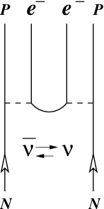
Figure 1: Neutrinoless double beta decay-schematic representation.

This process is associated with a second order element of the $S$ matrix and the related amplitude, here denoted by, $T_{0\nu\beta\beta}$, is given by

$$T_{0\nu\beta\beta}=W^{\mu}\,W^{\eta}[\bar{u}_{e}\gamma_{\mu}(1+\gamma_{5})u_{\nu_{e}}][\bar{u}_{e}\gamma_{\eta}(1+\gamma_{5})u_{\nu_{e}}]\,.$$ (152)

In order to bring in the virtual neutrino line in Eq. (152), one makes use of the following identity:

$$\bar{u}_{e}\gamma_{\eta}(1+\gamma_{5})u_{\nu_{e}} = \overline{\left((u_{e})^{c}\right)^{c}}\gamma_{\eta}(1+\gamma_{5})\left((u_{\nu_{e}})^{c}\right)^{c}$$ (153)

$$= \bar{u}_{\nu_{e}}\,[-\gamma_{\mu}(1-\gamma_{5})]\,v_{e}\,.$$

The latter expression is obtained by making use of the relations, $\gamma_{0}\gamma_{\mu}^{\ast}=\gamma_{\mu}\gamma_{0}$, $\gamma_{2}\gamma_{\mu}=-\gamma_{\mu}^{\ast}\gamma_{2}$, $\gamma_{\mu}^{t}=-\gamma_{\mu}$, the anti-commutation relations between the Dirac matrices, with ${}^{\prime\prime}t^{\prime\prime}$ labeling the transposed. With that Eq. (152) takes the form

$$T_{0\nu\beta\beta} = W^{\mu}\,W^{\eta}\frac{1}{p_{\nu_{e}}^{2}-m_{\nu_{e}}^{2}}L_{\mu\eta}\,,$$

$$L_{\mu\eta} = \,\bar{u}_{e}\gamma_{\mu}(1+\gamma_{5})\Pi^{\nu_{e}}\,[-\gamma_{\mu}(1-\gamma_{5})]\,v_{e}\,,$$

$$\Pi^{\nu_{e}} = \sum u_{\nu_{e}}\bar{u}_{\nu_{e}}\,.$$ (154)

Here we suppressed ${}^{\prime\prime}h^{\prime\prime}$ labeling of the Dirac spinors in order not to overload notations so that $\sum$ in $\Pi_{\nu_{e}}$ means summation over spin projections. Finally, $|L_{\mu\eta}|^{2}$ can be converted to a trace in the standard way as

$$|L_{\mu\eta}|^{2}={\Big{[}}\bar{u}_{e}\gamma_{\mu}(1+\gamma_{5})\Pi^{\nu_{e}}\,\gamma_{\eta}(1-\gamma_{5})\,v_{e}{\Big{]}}\,$$

$${\Big{[}}\bar{u}_{e}\gamma_{\lambda}(1+\gamma_{5})\Pi^{\nu_{e}}\,\gamma_{\delta}(1-\gamma_{5})\,v_{e}{\Big{]}}^{\dagger}\,$$

$$=tr{\Big{[}}\Pi^{u_{e}}\gamma_{\mu}(1+\gamma_{5})\Pi^{\nu_{e}}\gamma_{\eta}(1-\gamma_{5})\Pi^{v_{e}}$$

$$\gamma_{\delta}\gamma_{0}(1+\gamma_{5})\Pi^{\nu_{e}}\gamma_{0}(1-\gamma_{5})\gamma_{\lambda}{\Big{]}}$$

$$=tr{\Big{[}}\Pi^{u_{e}}\gamma_{\mu}\frac{2m_{\nu_{e}}}{p_{\nu_{e}}^{2}}\gamma_{\eta}(1-\gamma_{5})\Pi^{v_{e}}\gamma_{\delta}\gamma_{0}\frac{2m_{\nu_{e}}}{p_{\nu_{e}}^{2}}\gamma_{0}(1-\gamma_{5})\gamma_{\lambda}{\Big{]}} \,.$$

In the latter equation the squared neutrino mass ($m_{\nu_{e}}^{2}$) was neglected compared to the squared neutrino momentum, $p_{\nu_{e}}^{2}$, with the well known result

$$(1+\gamma_{5}){\Pi^{\nu_{e}}}\gamma_{\eta}(1-\gamma_{5})=\frac{2m_{\nu_{e}}}{p_{\nu_{e}}^{2}}\gamma_{\eta}(1-\gamma_{5})\,.$$ (156)

Now we calculate above trace within the scenario of the previous section. To do so, one has to perform in Eq. (LABEL:04_bb) the replacements $\gamma_{\mu}\to\Gamma_{\mu}$, $u_{e}\to U_{e}$, $v_{e}\to V_{e}$, $u_{\nu_{e}}\to\Lambda^{S/A}_{k}$, and

$$\Pi^{\nu_{e}}\to\frac{1}{2m}\left(\begin{array}[]{cc}m1_{4}&-ip\!\!\!/\\ ip\!\!\!/&m1_{4}\end{array}\right)\left(\begin{array}[]{cc}0_{4}&-i1_{4}\\ i1_{4}&0_{4}\end{array}\right)\,.$$ (161)

Our calculation shows that the $0\nu\beta\beta$ trace contains $\widetilde{\Gamma_{8}}^{2}$ which is the $(8d)$ identity matrix. In effect, one recovers Eq. (LABEL:04_bb) and the well known proportionality of the $0\nu\beta\beta$ trace to the square of the neutrino mass. Therefore, the Majorana calculus does not alter results of the Dirac theory of the neutrinoless double beta decay.

5 Summary.

We constructed two types of truly neutral spin-1/2 quantum fields that differ by the $C$ parity of the underlying momentum space Majorana spinors, real versus imaginary, a property that shows up as a difference in the symmetry of the corresponding Majorana mass matrices–real symmetric versus imaginary anti-symmetric. We exploited above fields to calculate traces of single and neutrinoless double beta decays. Compared to standard phenomenology, the neutrinoless double beta decay remains unaltered for both fields. The result extends also to one-gaugino exchange as long as the virtual fermion line in Fig. 1 can be also a massive gaugino.

In single beta decay, we observed a cancellation of the neutral fermion mass in the trace, in the case of the Majorana field with the anti-symmetric mass matrix.

The latter option opens the curious possibility to have a neutral fermion theory at hand that allows (polarized) tritium $\beta$ decay Bonn to drive the neutrino mass closer to zero compared to neutrino oscillation– , and $0\nu\beta\beta$ measurements, thus providing an intriguing and in principle experimentally testable signature for a non-trivial impact of momentum space Majorana spinors on phenomenology.

6 Acknowledgments.

Work supported by Consejo Nacional de Ciencia y Tecnologia (CONACyT) Mexico under grant number C01-39820.

References

• (1) M.E. Peskin, D.V. Schroeder, An Introduction to Quantum Field Theory (Westview Press, N.Y. 1995) pp. 68-76.
• (2) E. Majorana, Nuovo Cimento 14, (1937) 171.
• (3) B. Kayser, F. Gibat-Debu, F. Perrier, The Physics of Massive Neutrinos, Lecture Notes in Physics Vol. 25 (World Scientific, Singapore, 1989).
• (4) E.D. Commins, P.H. Bucksbaum, Weak Interactions of Leptons and Quarks (Cambridge Univ. Press, 1983).
• (5) B. Kayser, Phys. Rev. D 30, (1984) 1023.
• (6) M. Kirchbach, C. Jasso, L. Noriega, Neutral fermion phenomenology with Majorana spinors, E-Print Archive: hep-ph/0310297.
• (7) P. Ramond, Field Theory: A Modern Primer (Addison-Wesley, Redwood City, California, 1989) p. 20.
• (8) Fayyazudin, Riazuddin, A Modern Introduction to Particle Physics (World Scientific, Singapore, 2000) pp. 325-330, Appendix A.8.
• (9) Stefan Pokorski, Gauge Field Theories, 2nd edition (Cambridge Univ. Press, 2000,) pp. 26-29.
• (10) S.M. Bilenky, B.M. Pontekorvo, Phys. Rep. 42, 224 (1978).
• (11) S. Esposito, N. Tancredi, Eur. Phys. J. C 4, 221 (1998).
• (12) J. Hladik, Spinors in Physics (Springer-Verlag, N.Y., 1999).
• (13) M. Kirchbach, D.V. Ahluwlaia, Phys. Lett. B 529, 124 (2002).
• (14) D.V. Ahluwalia, Int. J. Mod. Phys. A 11, 1855 (1996); D.V. Ahluwalia, T. Goldman, M.B. Johnson, Acta Phys. Pol. B 25, 1267 (1994).
• (15) V. V. Dvoeglazov, Int. J. Theor. Phys. 34, 2467 (1995).
• (16) Judah Eisenberg, Walter Greiner, Nuclear Theory, Vol. 2 (North Holland Publ. Comp., Amsterdam-London, 1970), Chapt. 9.
• (17) J. Bonn et al., Nucl. Phys. B 91, 273 (2001); J. Bonn, in Particles and Fields, edited by  J.L. Diaz-Cruz, J. Engelfried, M. Kirchbach, M. Mondragon, AIP Conf. Proc. 623, 189 (2002).