Conical Flow induced by Quenched QCD Jets

Abstract

Quenching is a recently discovered phenomenon in which QCD jets created in heavy ion collisions deposit a large fraction or even all their energy and momentum into the produced matter . At RHIC and higher energies, where that matter is a strongly coupled Quark-Gluon Plasma (sQGP) with very small viscosity, we suggest that this energy/momentum propagate as a collective excitation or “conical flow”. Similar hydrodynamical phenomena are well known, e.g. the so called sonic booms from supersonic planes. We solve the linearized relativistic hydrodynamic equations to detail the flow picture. We argue that for RHIC collisions the direction of this flow should make a cone at a specific large angle with the jet, of about $70^{o}$, and thus lead to peaks in particle correlations at the angle $\Delta\phi=\pi\pm 1.2$ rad relative to the large-$p_{t}$ trigger. This angle happens to match perfectly the position of the maximum in the angular distribution of secondaries associated with the trigger recently seen by the STAR and PHENIX collaborations. We also discuss briefly possible alternative explanations and suggest some further tests to clarify the mechanism.

1 Introduction

Jet quenching is an important phenomenon, predicted in a number of papers [1] and recently observed at RHIC [2]. The main research has been so far related to the calculation of the energy loss $dE/dx$ of the fastest parton, and focused on a kind of tomography of the produced matter. In this work, however, we focus on a different question: Where does the energy of the quenched jets go? We point out that as the hydrodynamical description of sQGP excitations works well, it should be used to predict how collective flow would develop, after a local deposition of energy and momentum. As we will see below, it will be a coherent source of sound waves in conical form.

In what follows, we would like to treat two different types of energy losses separately : (i) the radiative losses, producing relativistic gluons in the forward direction; and (ii) the scattering/ionization losses, which deposit energy and momentum directly into the medium, as well as radiative losses of gluons at rather large angles (see Discussion section). Such gluons are rather soft and are promptly absorbed by the medium.

The study of radiative losses were started in [3], then corrected for the destructive interferences (the so-called Landau-Pomeranchuck-Migdal or LPM effect) in [4]. For a recent brief summary, see also [5]. Although it is the dominant mechanism for quenching hard ($z\sim 1$) fragmenting hadrons, in our problem the second type of losses are more important because the primary parton and the radiated gluons all move with speed close to the speed of light and are treated as one object.

Elastic energy losses were first studied by Bjorken[1], while those due to “ionization” of bound states in sQGP were recently considered by Shuryak and Zahed [6]. These mechanism deposit additional energy, momentum and entropy into the matter. (Like for delta electrons in ordinary matter, this excitation kicks particles mostly orthogonal to the jet direction.) It is their combined magnitude, $dE/dx=2-3\,GeV/fm$, the one we will use below. Even at such loss rates, a jet passing through the diameter of the fireball, created in central Au-Au collisions, may deposit up to 20-30 GeV, enough to absorb the jets of interest at RHIC.

Let us start our discussion of associated collective effects by recalling the energy scales involved. While the total CM energy in a Au-Au collision at RHIC is very large (about 40 TeV) compared to the energy of a jet (typically 5-20 $\,GeV$), the jet energy is transverse. The total transverse energy of all secondaries per one unit of rapidity is $dE_{\perp}/dy\sim 600\,GeV$. Most of it is thermal, with only about 100 GeV being related to collective motion. Furthermore, the so called elliptic flow is a $\sim 1/10$ asymmetry and therefore it carries energy $\sim 10\,GeV$ which is comparable to that lost by jets. Since elliptic flow was observed and studied in detail, we conclude that conical flow should be observable as well. (In order to separate the two, it is beneficial to focus first on the most central collisions, where the elliptic flow is as small as possible.)

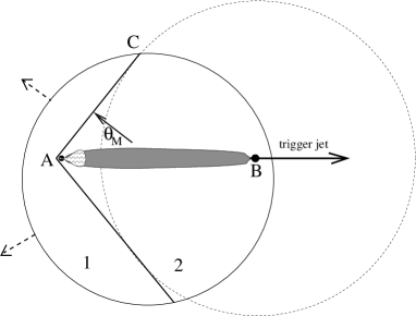
Figure 1: A schematic picture of flow created by a jet going through the fireball. The trigger jet is going to the right from the origination point (the black circle at point B) from which sound waves start propagating as spherical waves (the dashed circle). The companion quenched jet is moving to the left, heating the matter and thus creating a cylinder of additional matter (shaded area). The head of the jet is a “nonhydrodynamical core” of the QCD gluonic shower, formed by the original hard parton (black dot A). The solid arrow shows a direction of flow normal to the shock cone at the angle $\theta_{M}$, the dashed arrows show the direction of the flow after the shocks hit the edge of the fireball.

Fig.1 explains a view of the process in a plane transverse to the beam. Two oppositely moving jets originate from the hard collision point B. Due to strong quenching, the survival of the trigger jet biases it to be produced close to the surface and to move outward. This forces its companion to move inward through matter and to be maximally quenched. The energy deposition starts at point B, thus a spherical sound wave appears (the dashed circle in Fig.1 ). Further energy deposition is along the jet line, and is propagating at the speed of light, till the leading parton is found at point A at the moment of the snapshot.

As is well known, the interference of perturbations from a supersonically moving body (such as a supersonic jet plane or a meteorite) creates a conical flow behind the shock waves. Similar flow was discussed in Refs[7] for shocks in cold nuclear matter, in which compression up to QGP production takes place. Unfortunately, experiments have shown that nuclear matter is too dilute and dissipative to make shocks: but discoveries made at RHIC let us be more optimistic in the sQGP case we consider now [8].

The angle $\theta_{M}$ defined in the figure is given by a simple geometrical condition: the distance traveled by the jet during the proper time interval $\tau$ is $AB=c\tau$, while the one traveled by the wave is

$$CB=\int_{0}^{\tau}c_{s}(t)dt~{}~{}\Longrightarrow~{}~{}cos\theta_{M}={1\over c\tau}\int_{0}^{\tau}c_{s}dt~{}.$$ (1)

We use the speed of sound since, apart from the region close to the head of the object [9], the shock waves are weak and thus they move with the speed of sound (we use units in which c=1.)

The region near the head of the jet, which we will refer to as a “non-hydrodynamical core”, will not be discussed in this work. Let us just mention that near point B, where the jet is produced, it consists of an “undressed” hard parton only. However, as it is constantly emitting gluons, which emit new ones etc., the whole shower is a complicated nonlinear phenomenon which should obviously be treated via the tools of quantum field theory [10]. As found in [4], the multiplicity of this shower grows nonlinearly with time, so eventually the core may become a macroscopic body, providing a large perturbation of the matter. From the hydrodynamical point of view, its size is limited from below by the dissipative “sound attenuation length” $\Gamma_{s}=(4/3)\eta/(\epsilon+p)$, with $\eta$ being the shear viscosity.

A shaded region in Fig.1 consists of “new matter” related to the entropy produced in the process $dS/dx$, which can be calculated only with dissipative dynamics in the near zone, which we do not attempt in this work. Matter is expected to get equilibrated soon, and thus the radius of the cylinder $R_{c}$ of new matter can be estimated as $dS/dx=s(T)\pi R_{c}^{2}$. As is well known, a constant size cylinder does not emit any sound.

2 Linearized Hydrodynamics

The hydrodynamical equations we use are simpler than those used in Refs[7] since we will consider that the total energy-momentum density deposited by the jets is a small perturbation compared to the total energy of the medium. This allows us to linearize the problem. The approximation breaks down close to the jet, where we will not describe the hydrodynamic fields. We will use cylindrical coordinates with $x$ and $r$ parallel and perpendicular to the jet axis, respectively. We will also assume that the perturbed medium is homogeneous and at rest.

In the linearized approximation we define the following quantities in terms of perturbations of the stress energy tensor:

$$\epsilon=\delta T^{00}~{}~{},~{}~{}g^{i}=\delta T^{0i}~{}.$$ (2)

The remaining non-zero components of the stress tensor [11] are:

$$T^{ij}=c^{2}_{s}\epsilon\delta^{ij}-\frac{\eta}{\epsilon_{0}+p_{0}}\left<\partial^{i}g^{j}\right>~{}~{},~{}~{}\left\langle\partial^{i}g^{j}\right\rangle=\partial^{i}g^{j}+\partial^{j}g^{i}-\frac{2}{3}\delta^{ij}\partial_{i}g^{i}~{}.$$ (3)

Here we have used $\frac{\partial p}{\partial e}=c^{2}_{s}$ and recall that in the linearized approximation the velocity field is $v^{i}=\frac{g^{i}}{\epsilon_{0}+p_{0}}$; $\epsilon_{0}$ and $p_{0}$ are the energy density and pressure of the unperturbed medium.

The energy and momentum conservation equations $\partial_{\mu}\delta T^{\mu\nu}$, can be written in Fourier space, where we observe that if we define $\vec{g}=g_{\scriptstyle\rm L}\frac{\vec{k}}{k}+\vec{g_{\scriptstyle\rm T}}$ (where L ant T stand for longitudinal and transverse respectively), the linearized hydro equation decouples as:

$$\partial_{t}\epsilon+ikg_{\scriptstyle\rm L}=0~{},$$

$$\partial_{t}g_{l}+ic^{2}_{s}k_{\scriptstyle\rm L}\epsilon+\frac{\eta}{\epsilon_{0}+p_{0}}\frac{4}{3}k^{2}g_{\scriptstyle\rm L}=0~{},$$ (4)

$$\partial_{t}\vec{g_{\scriptstyle\rm T}}+\frac{\eta}{\epsilon_{0}+p_{0}}k^{2}\vec{g_{\scriptstyle\rm T}}=0~{}.$$ (5)

The system of equations (2) describes sound waves (propagating modes). Equation (5) is the diffusion equation and is not propagating. Only the sound waves will form the Mach cone.

3 Initial conditions

The initial conditions are set by the process of thermalization of the energy and momentum lost by the jet. This complex process should take place at distances of order $\Gamma_{s}$ from the production point. As $\Gamma_{s}$ is also the minimal size of the liquid cells, we will simply consider that there is a variation of $T^{\mu\nu}$ at the position of the particle.

If we consider an infinitesimal displacement $dt_{0}$ of the high energy particle (moving with the speed of light) in the $x$ direction at the point $(t_{0},t_{0},\vec{0})$, we need to specify the infinitesimal variation of the fields $\epsilon_{dt_{0}}(t=t_{0},\vec{x})$, $\vec{g_{dt_{0}}}(t=t_{0},\vec{x})$. Due to the symmetries of the problem, the most general expression for those functions is:

$$\epsilon_{dt_{0}}(t=t0,\vec{x})=e_{0}(z,r)~{}~{},~{}~{}\vec{g}_{dt_{0}}(t=t0,\vec{x})=g_{0}(z,r)\delta^{ix}+\vec{\partial}g_{1}(z,r)~{}.$$ (6)

As argued before $e_{0}$, $g_{0}$ and $g_{1}$ are some functions with characteristic scale $\sigma\sim\Gamma_{s}$. The exact expression for these functions depends on the details of the thermalization process. As we do not know these details, we will need to make certain assumptions about the different functions that appear in (6). In general, one may consider two different scenarios of matter excitation:

Scenario 1 in which local deposition of energy and momentum is described by the first terms in (6), $e_{0}$ and $g_{0}$. This imposes a constraint in (6):

$$\int d^{3}x\epsilon_{dt_{0}}(t=t0,\vec{x})=\frac{dE}{dx}dt_{0}~{}~{},~{}~{}\int d^{3}xg^{x}{dt_{0}}(t=0,\vec{x})=\frac{dP}{dx}dt_{0}~{},$$ (7)

where $\frac{dE}{dx}$ and $\frac{dP}{dx}$ are an input. In this case $g_{1}=0$. These simple initial conditions, however, excite the “diffuson mode” and thus be discarded later.

Scenario 2 in which the excitation is due to the gradient term $g_{1}$ in (6), with $\epsilon_{0}=0$ and $\vec{g_{0}}=0$. The deposition of energy and momentum in this case comes from the second order effects. The normalization of such solutions are better done at large distances, via the energy flow and the momentum flow through a large cylinder. As we show below, this generates the conical solution with sound excitation.

The empirical fact that the second scenario describes the data and the first one does not obviously provides some insights about the excitation mechanisms, but we would not speculate about them now.

4 Solutions

In order to solve (2) and (5) with the initial condition (6), we will calculate the corresponding kernels, that is, we will set the functions appearing in (6) to be $\delta$-functions. Following the standard procedure, we convolute these kernels with some parametrization for $e_{0}$, $g_{0}$, and $g_{1}$:

$$T^{0\mu}(x)=\int d^{3}y\left(K^{\mu}_{e}\left(x-y\right)e_{0}(y)+K^{\mu}_{g_{0}}\left(x-y\right)g_{0}(y)+K^{\mu}_{g_{1}}\left(x-y\right)g_{1}(y)\right)~{}.$$ (8)

and integrate over the trajectory of the particle.

Scenario 1. In this case we only consider point like excitation in $e_{0}$, $g_{0}$. Keeping terms to order $O(\Gamma_{s}^{2})$ we find the following 4-vector kernels:

$$K^{\mu}_{e}=\sum_{i=\pm}\left(\frac{-1}{4\pi r}\partial_{r}P_{i}(\Gamma_{s}),\partial^{k}\frac{c_{s}}{4\pi r}iP_{i}(\Gamma_{s})\right)~{},$$ (9)

$$K^{\mu}_{g_{0}}=\sum_{i=\pm}\left(\partial_{x}\frac{iP_{i}(\Gamma_{s})}{4\pi c_{s}r},\partial^{k}\partial_{x}\frac{-\int^{r}_{0}P_{i}(\Gamma_{s})}{4\pi r}\right)+\left(0,\partial^{k}\partial_{x}\frac{2\int^{r}_{0}P(\frac{3}{2}\Gamma_{s})}{4\pi r}+\delta^{kx}\frac{e^{\frac{-r^{2}}{2\frac{3}{2}\Gamma_{s}t}}}{\left(2\pi\frac{3}{2}\Gamma_{s}t\right)^{3/2}}\right)~{}.$$ (10)

Where $r=|\vec{x}-\vec{x}(t_{0})|$ is the distance from the observation point to the jet position and we have defined the functions:

$$P_{\pm}(\Gamma_{s})=\frac{1}{\sqrt{2\pi\Gamma_{s}t}}e^{-\frac{(r\pm c_{s}t)^{2}}{2\Gamma_{s}t}}~{}~{},~{}~{}P(\frac{3}{2}\Gamma_{s})=\frac{1}{\sqrt{2\pi\frac{3}{2}\Gamma_{s}t}}e^{-\frac{r^{2}}{2\frac{3}{2}\Gamma_{s}t}}~{}.$$ (11)

The second term in (10) is the (Fourier transform of the) so called diffusion mode (or diffuson) (5). It creates a dissipating flow of matter comoving with the jet that remembers the location of deposition of momentum. As we will show below, this type of excitation leads to a forward peak in the final spectrum filling up the Mach cone (related to (9) and the first term in (10)).

These kernels should be convoluted with the initial distributions. We take a simple parametrization (Gaussian) that fulfills the requirement (7):

$$e_{0}(t=t_{0},\vec{x})=\frac{dE}{dt_{0}}dt_{0}\frac{e^{-\frac{(\vec{x}-t_{0}\hat{x})^{2}}{2\sigma^{2}}}}{(2\pi\sigma^{2})^{3/2}}~{}~{},~{}~{}g_{0}(t=t_{0},\vec{x})=\frac{dP^{x}}{dt_{0}}dt_{0}\frac{e^{-\frac{(\vec{x}-t_{0}\hat{x})^{2}}{2\sigma^{2}}}}{(2\pi\sigma^{2})^{3/2}}\delta^{kx}~{}.$$ (12)

Scenario 2 Following the same procedure we find the 4-kernel:

$$K^{\mu}_{g_{1}}=\sum_{i=\pm}\left(\frac{i}{4\pi c_{s}r}\partial^{2}_{r}P_{i}(\Gamma_{s}),\partial^{k}\frac{-1}{4\pi r}\partial_{r}P_{i}(\Gamma_{s})\right)~{},$$ (13)

where the definitions are the same as in (9) and (10). Note that as claimed, we now find a propagating solution, the sound wave.

For example, let us assume a simple parametrization for the initial source:

$$g_{1}(t=t_{0},\vec{x})\sim e^{-\frac{(\vec{x}-t_{0}\hat{x})^{2}}{2\sigma^{2}}}~{}.$$ (14)

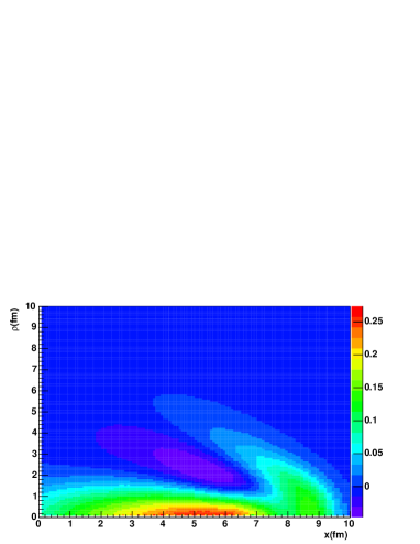
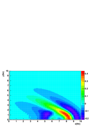
Figure 2: Velocity field $v_{x}$ created by a jet moving along the $\hat{x}$ direction ($c^{2}_{s}=1/3$, $\Gamma_{s}=1/(4\pi T)$, $\sigma=\Gamma_{s}$). The jet is assumed to disappear at $t=7$ fm while the spectrum calculated at $t=10$ fm. The two figures (a) and (b) are for scenarios 1 and 2, respectively. The values of the parameters are arbitrary. Note that in (a) matter moves preferentially along the $\hat{x}$ direction, while in (b) it is in the Mach direction (1).

In Fig.2 we show the velocity field along the jet axis generated by the high energy particles according to both models of the initial conditions. In Fig. 2(a) we can observe the effect of the diffuson as a maximum in the velocity along the $\hat{x}$ axis, where the jet propagates. In Fig. 2(b) such maximum does not exist, as there is no excitation of the diffusion mode. We also observe in both cases the sound wave, that is more prominent in the second case. Note also that in both cases we have positive and negative velocities, that is, matter moving outward and inward (as it should be due to conservation of matter).

5 Spectrum

We use the previous hydrodynamic fields to calculate the final spectrum induced by the jet. To do so, we use the standard Cooper-Fry prescription. As our initial medium is static, we use fixed time freeze-out (neglecting the effect of the perturbation on the freeze out):

$$\frac{dN}{d^{3}p}=\int_{V}d^{3}Ve^{-\frac{E}{T_{frzt}}+\delta}~{}~{},~{}~{}\delta=\frac{E}{T_{frzt}}\frac{\delta T}{T_{frzt}}+\frac{\vec{p}\vec{v}}{T_{frzt}}~{},$$ (15)

where V is the volume of the fireball and $T_{frzt}$ is the freeze-out temperature. According to our approximation, we expand the exponent to first order in the perturbation. We can now discuss two opposite regimes in the spectrum:

Low energy particles $E\sim T_{frzt}$. In this region we can expand the exponential in (3) and express the spectrum in terms of the energy and momentum deposited (to first order):

$$\frac{dN}{d^{3}p}=e^{-\frac{E}{T_{frzt}}}\left(V+\frac{E}{T_{frzt}}\frac{E_{dep}}{\epsilon_{0}+p_{0}}+\frac{\vec{P}}{T_{frzt}}\frac{\vec{P}_{dep}}{\epsilon_{0}+p_{0}}\right)~{}.$$ (16)

One finds that soft particles are insensitive to the particular shape of the flow field and their angular dependence is just a cosine of the relative angles of the observed particle and the jet.

High energy particles $E>>T_{frzt}$ which compensates the smallness of the flow velocity. The integral is now dominated by the maximum of the exponent. Thus, only the points of maximum modifications of hydrodynamic fields contribute to the final spectrum. It is clear then that in the scenario 1 the diffusion mode totally dominates the spectrum and there are no angular correlations related to the speed of sound. However, in the second scenario one does not excite that mode, and the final spectrum do reflect the shape of the sonic disturbance.

In order to illustrate the effect of the modification of the final particle production due to a jet moving with $y=0$ and $\phi=\pi$, we show in Fig.3 the normalized spectrum defined as follows:

$$C=\frac{1}{Q}\frac{dN}{dyd^{2}p_{t}}(y=0,p_{t},\phi)~{}~{},~{}~{}Q=\int^{2\pi}_{0}d\phi\frac{dN}{dyd^{2}p_{t}}(y=0,p_{t},\phi)~{}.$$ (17)

We observe that, as claimed, the effect of the diffusion mode hides the Mach cone in the final production. As a consequence, we do not observe such a structure in fig Fig.3(a); we do observe it, however, in Fig.3(b), where such mode is not excited.

The parameters in Fig.3 are arbitrary (with the exception of $\Gamma_{s}$, which is set to its minimal bound [12]), and are chosen as a matter of illustration. Let us remark that these spectra are very sensitive to the value of $\Gamma_{s}$, which could provide a experimental constraint on its value, provided a correct understanding of the deposition process.

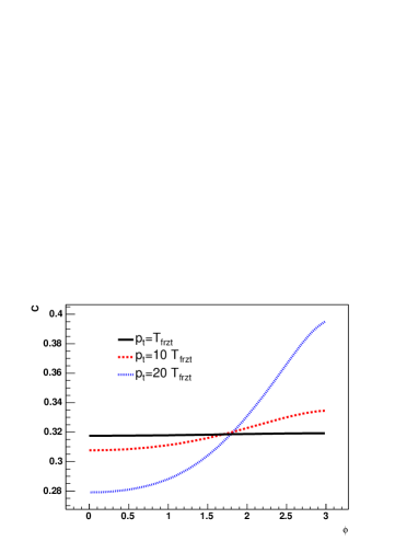
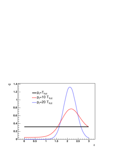
Figure 3: The normalized spectrum of associated secondaries versus the azimuthal angle $\phi$. Three curves are for different $p_{t}$ at $y=0$ for $c^{2}_{s}=1/3$, $\Gamma_{s}=1/(4\pi T)$, $\sigma=\Gamma_{s}$. Note the different scales. The jet disappears completely at $t=7$ fm while the spectrum is calculated at $t=10$ fm. The two figures (a) and (b) are for scenarios 1 and 2, respectively.

6 How can the effect be observed?

The most important feature of conical flow is its direction, which is normal to the shock front and thus making the so called Mach angle (1) with the jet direction, determined basically by the speed of sound in matter. So one can conclude that quenched jets must be accompanied by a cone of particles with the opening angle $\theta_{M}$. This cone angle should be the same for any jet energy (in contrast to radiation angles, which are shrinking at high energy).

The appropriate value for the speed of sound is a time-weighted average of three stages: (i) the QGP phase ($c_{s}\approx 1/\sqrt{3}$), (ii) the mixed phase $c_{s}\approx 0$ and (iii) the hadronic or “resonance gas” stage, with $c_{s}\approx\sqrt{.2}$ [13]. For RHIC we found the time-weighted average to be $\bar{c}_{s}\approx.33$. We thus conclude that in this case the emission angle of the conical flow should be at angles about 70 degrees relative to the jet, or in radians

$$\theta_{emission}=\pi\pm arccos(\bar{c}_{s}/c)\approx 1.9,4.3.$$ (18)

The first measurements of interest to this issue have been made by the STAR collaboration [14], [15] which studied two particle correlations in which the trigger particle has $4<p_{t}<6~{}GeV$, while the associated particles have basically all momenta (in fact $0.15<p_{t}<4~{}GeV$ ). At $\Delta\phi=0$ one finds a peak due to particles from the triggered jet, while particles from the companion jet should result in a peak at $\Delta\phi=\pi$. Such peak is clearly seen in pp collisions, in which no matter is present: but in Au-Au collision one finds instead a double-peaked distribution with a $minimum$ at the original jet direction $\Delta\phi=\pi$. Remarkably this value $\pi\pm 1.2$ nicely agrees with the observed positions of the two maxima of the distribution of secondaries.

After submission of our paper in the preprint form, two more important observations have been made, both discussed at this workshop [15],[16].

The PHENIX collaboration have shown [16] correlation function in which the companion particle is harder than the average $p_{t}>1\,GeV$. They also reported data for 6 centrality classes and in all of them (but the most peripheral one) there is a minimum at 180^o and even sharper peaks at the same angle as we predict. We also remark that our results in Fig.3(b) for $p_{t}=10T_{frzt}$ ($T_{frzt}=100$ MeV) are similar to the correlation functions in [16].

The STAR collaboration also reported [15] the associated particle mean $\left<p_{t}\right>(\phi)$, which also displays maxima away from $\phi=\pi$, where one finds a clear minimum. This fact strongly supports our explanation of the peaks by conical flow. The fact that at 180^o the mean $p_{t}$ of associated secondaries is consistent in magnitude with the mean transverse momentum in the average background events means that in the experimental conditions the inward-moving jet is completely quenched by freeze-out and no contribution from the “nonhydro core” is visible in the data.

Unfortunately, we can only see a projection on $\Delta\phi$ because the distribution in rapidity of the associated jet is very wide, wiping out another projection of the cone. One could think that this wide rapidity distribution could also wipe out the double peak structure in the final two particle correlation. Even though the full hydrodynamic problem should be solved, we can give here an argument by which this does not happen. For that we assume boost invariance of the medium and that the rapidity ($y_{j}$) distribution of the away jet is flat. We will also assume that particles are formed in a cone around the jet axis. It is clear then, that in a frame with rapidity $y_{j}$ (where the away side jet is transverse) the spectrum of those particles can only depend on the momentum of the particle ($p_{j}$) and its angle with respect to the jet ($\theta^{*}$). We assume also that this dependence factorizes and that the dependence in $\theta^{*}$ is a very narrow function of angle $\theta_{c}^{*}$ (the cone opening angle). Thus, the spectrum of particles produced by a jet with rapidity $y_{j}$ can be written as,

$$E\frac{dN}{d^{3}p}=P(y_{j})dy_{j}f_{p}(p_{j})\delta(\cos(\theta^{*})-\cos(\theta^{*}_{c}))~{},$$ (19)

where $P(y_{j})$ is the probability of finding a jet with such rapidity. We will concentrate now on the spectrum of particles at mid rapidity (y=0) in the lab frame. Boosting back to this frame, we find $p_{j}=p_{t}\cosh(y_{j})$ and $\cos(\phi)=\cos(\theta^{*})\cosh(y_{j})$, where $p_{t}$ and $\phi$ are the transverse momentum and azimuthal angle respectively. Thus:

$$\delta(\cos(\theta^{*})-\cos(\theta^{*}_{c}))=\frac{\delta(y_{j}-y^{*}_{j})}{\cos(\theta^{*}_{c})\sqrt{1-\frac{\cos^{2}(\theta^{*}_{c})}{\cos^{2}(\phi)}}}~{}~{},~{}~{}\cosh(y^{*}_{j})=\frac{\cos(\phi)}{\cos(\theta^{*}_{c})}~{}.$$ (20)

Upon integration on $y_{j}$ (assuming P constant) we find

$$E\frac{dN}{d^{3}p}=Pf_{p}(p_{t}\frac{\cos(\theta^{*}_{c})}{\cos(\phi)})\frac{1}{\cos(\theta^{*}_{c})\sqrt{1-\frac{\cos^{2}(\theta^{*}_{c})}{\cos^{2}(\phi)}}}~{},$$ (21)

which is clearly a peaked distribution around $\phi=\pm\theta^{*}_{c}$. What is more, $f_{p}$ should be a steeply falling function (exponential in our case) of its argument, which depletes more the fill up. A width on the angular dependence will modify the result but a quantitative answer to this effect requires further study.

7 Discussion:

We have considered an idealized case of homogeneous matter at rest. The determination of the exact shape of this cone for real collisions is not simple. It is of course just a technical matter to include the superposition of radial, elliptic and conical flows in a single hydro simulation. The open issue, however, would be the inclusion of viscosity at the hadronic stage, which is not supposed to be small. Presumably, as for elliptic flow, the use of a hadronic cascade afterburner would provide more realistic results.

When the conical solution reaches the surface of the fireball or the freeze-out surface, the energy stored in outward (positive) flow would continue to move in the same direction, while the inward (negative) one would be absent. As the shock moves into the lower density region near the edge, energy conservation would force its amplitude to grow, like do the ocean waves approaching the beach, or the whip motion near its thin end. Furthermore, if the jet is energetic enough to punch through, the regions where cones reach the edge consist of two separated regions (circular rings if the jet goes via the diameter) moving toward each other and eventually colliding, where the cone and the fireball surface are tangent.

We have seen that the choice of initial condition is very important for the final result, as the excitation of the diffusion modes may hide the cone formation in the final spectrum. We have presented two different scenarios that are, in a sense, opposite limits, as in one of then we do not excite this mode. The appearance of such mode in the actual initial conditions, will lead to some (or even complete) fill up of the cone in the two particle correlations. This fill up, is also expected for high energy particles, in which the jet punches through. This is however a completely different mechanism from the previous, which will lead to a very different $p_{t}$-spectrum of the associated particles (exponential in the first, power law in the second)

Can there be an alternative explanation of the high-angle maxima observed? Another two different mechanisms have been proposed:

Large angle gluon radiation It has been argued [17] that QCD radiation calculated with Landau-Pomeranchuck-Migdal effect included, may have a maximum at large angles, similar to the Mach angle we discuss. Those calculations, however, used static (infinitely massive) scatterers. A simple kinematical calculation reveals that in the limit in which the energy of the jet is much larger than the energy of the target, any angular distribution of radiation in the center of mass frame leads to a forwardly peaked distribution in the rest frame of the target. In spite of this, even if one could argue that the scatterers were heavy, the same calculations presented in [17] cannot reproduce a double peak structure. In fact, the gluon distribution obtained in [17] are such that after integrating over the (flat) rapidity distribution of the associated jet, any double peak structure would disappear in the final correlation function.

Deflection of the jet due to transverse expansion. This idea has been suggested in [18] and is similar to those in [19]. In this scenario, as the jet travels through the medium it changes its trajectory according to the direction of expansion of the medium it travels through. Thus, depending on the formation point of the jet, it will be deflected in a different direction with respect to the original axis (set by the triggered particle). Even though there are not quantitative estimates of this effect, we can establish one fundamental difference with respect to our scenario: particles are not produced in a cone around $\pi$, as jets are deflected in either direction with respect to the original one. Thus, in an event by event basis, the two particle correlations should peak either at angles smaller or bigger than $\pi$, and is the convolutions of all events which are the responsible for the double peak. This picture should be easily distinguished from ours via three particle correlations [20].

8 Summary:

We suggest that the lost energy of the quenched jets is not just absorbed by the heat bath, but appears in the form of hydrodynamical collective motion similar to known “sonic booms” in the atmosphere behind the supersonic jets. The reason for that is that QGP seems to be a near-perfect liquid, with remarkably small dissipative effects and robust collective flows. We argue that this should result in a cone of particles moving in the Mach direction (1). The first data on the particle distribution associated with the quenched jet (the away side from high energy hadron trigger) indeed show two peaks, with cone angles which agree well with our prediction.

We thank Stony Brook PHENIX group and especially B.Jacak for multiple discussions of the jet-related correlations which led us to this work. One of us (ES) thanks K.Filimonov for enlightening discussion at its early stage. We thank H.Stocker who pointed out to us his talks in which similar suggestions have been made. This work was partially supported by the US-DOE grants DE-FG02-88ER40388 and DE-FG03-97ER4014.

References

References

- [1] Bjorken J D , FERMILAB-PUB-82-059-THY \nonumAppel D A 1986 Phys. Rev. D 33 717 \nonumBlaizot J P and McLerran L D 1986 Phys. Rev. D 34 2739
- [2] Adcox K et al (PHENIX) 2002 Phys. Rev. Lett. 88 022301 \nonumAdler C et al (STAR) 2002 Phys. Rev. Lett. 89 202301 \nonumAdler S S et al (PHENIX) 2003 Phys. Rev. Lett. 91 072301 \nonumAdams J et al (STAR) 2003 Phys. Rev. Lett. 91, 172302
- [3] Gyulassy M and Plumer M 1990 Phys. Lett. B 243 432 \nonumWang X N, Gyulassy M and Plumer M, 1995 Phys. Rev. D 51 3436 \nonumFai G, Barnafoldi G G, M. Gyulassy, Levai P, Papp G, Vitev I and Zhang Y 2001 Preprint hep-ph/0111211
- [4] Baier R, Dokshitzer Y L, Peigne S and Schiff D 1995 Phys. Lett. B 345 277 \nonumBaier R, Dokshitzer Y L, Mueller A H and Schiff D 2001 JHEP 0109 033
- [5] Wang X N, 2004 Preprint nucl-th/0405017
- [6] Shuryak E V and Zahed I 2004 Preprint hep-ph/0406100
- [7] Chapline G F and Granik A 1986 Nucl.Phys. A 459 681 \nonumChapline G F and Granik A 1990 Nucl.Phys. A 511 747 \nonumRischke D H, Stocker H and Greiner W 1990 Phys.Rev. D 42 2283
- [8] After publication of our work as a preprint we learned that conical flow from jets was suggested by H.Stocker in several talks[21] previously
- [9] Since the velocity of the shock depends on its intensity, the cone should in fact be somewhat rounded near its top. This effect is ignored in the figure.
- [10] A charge/current distribution in the region near the jet is discussed in linear response theory in a recent paper by Ruppert and Muller [22]. Gluons and plasmons, with the dispersion laws suggested by pQCD at high T and lattice data, do generate Mach cones. We thus see no ground for the suggestion made by these authors
- [11] Teaney D 2003 Phys.Rev. C 68 034913
- [12] Policastro G, Son D T and Starinete A O 2001 Phys. Rev. Lett. 87 081601
- [13] Shuryak E V 1972 Yadernaya Fizika 16 395; R. Venugopalan and M. Prakash 1992 Nucl.Phys. A 546 718
- [14] Fuqiang Wang for STAR collaboration, (Quark Matter 2004), J.Phys.G 30 S1299-S1304,2004; Preprint nucl-ex/0404010
- [15] Fuqiang Wan for the STAR collaboration. (these proceedings)
- [16] Lacey R for the PHENIX collaboration (these proceedings)
- [17] Vitev I 2005 Preprint hep-ph/0501255
- [18] Fries R (these proceedings)
- [19] Armesto N, Salgado C A, Wiedemann U A 2004 Preprint hep-ph/0411341
- [20] Holtzmann W for the PHENIX collaboration (these proceedings)
- [21] Stocker H 2004 Preprint nucl-th/0406018
- [22] Ruppert J and Muller B 2005 Preprint hep-ph/0503158