OSU-HEP-04-13
Neutrino Oscillations in
Deconstructed Dimensions
Tomas Hällgrena†††E-mail: tomash@theophys.kth.se, Tommy Ohlssona‡‡‡E-mail: tommy@theophys.kth.se, and Gerhart Seidlb§§§E-mail: gseidl@susygut.phy.okstate.edu
aDivision of Mathematical Physics, Department of Physics
Royal Institute of Technology (KTH) – AlbaNova University Center
Roslagstullsbacken 11, 106 91 Stockholm, Sweden
bDepartment of Physics, Oklahoma State University
Stillwater, OK 74078, USA
Abstract
We present a model for neutrino oscillations in the presence of a deconstructed non-gravitational large extra dimension compactified on the boundary of a two-dimensional disk. In the deconstructed phase, sub-mm lattice spacings are generated from the hierarchy of energy scales between and the usual breaking scale . Here, small short-distance cutoffs down to can be motivated by the strong coupling behavior of gravity in local discrete extra dimensions. This could make it possible to probe the discretization of extra dimensions and non-trivial field configurations in theory spaces which have only a few sites, i.e., for coarse latticizations. Thus, the model has relevance to present and future precision neutrino oscillation experiments.
1 Introduction
There may be many ways to give a sensible short-distance definition of a model, which describes the Kaluza–Klein (KK) modes [1] of a compactified higher-dimensional gauge theory. One attractive possibility is offered by deconstructed [2] or latticized [3] extra dimensions. Deconstruction provides a new type of four-dimensional (4D) manifestly gauge-invariant and renormalizable field theories111For an early formulation in terms of infinite arrays of gauge theories, see Ref. [4]., which simulates in the infrared (IR) the physics of extra dimensions, and thus, yields a possible ultraviolet (UV) completion of higher-dimensional gauge theories [5]. In deconstruction, a bulk gauge symmetry is mapped onto copies of a 4D gauge group with bi-fundamental Higgs “link” fields connecting the neighboring groups. This becomes equivalent with treating the extra dimensional space as a transverse lattice [6], where the inverse lattice spacing is set by the vacuum expectation values (VEV’s) of the link fields. These models find a graphical interpretation in “theory space” [7], where the notion of extra dimensions has been translated into more general organizing principles of 4D field theories [8]. With this emphasis, the idea of theory space has stimulated the development of interesting theories in four dimensions, which need not be attributed any direct extra-dimensional correspondence at all.
Since deconstruction is formulated within conventional 4D field theory, one may now expect that a typical lattice cutoff naturally varies in the UV desert between and , i.e., in the energy range where usual effective field theories are defined. Indeed, if is, e.g., of the order the breaking scale , then a realistic neutrino phenomenology can arise [9], where small neutrino masses and bilarge leptonic mixing result from the lattice-link structure of the theory itself.222A recent attempt to obtain the quark mixing from deconstruction has been described in Ref. [10]. Generally, deconstructed non-gravitational extra dimensions always give a sensible effective field theory up to energy scales of the order , and hence, it seems that low cutoff scales are not particularly preferred in this case. However, for inverse lattice spacings above a TeV it will be difficult to test theory space models at low energies, unless the number of lattice sites is very large. On the other hand, cutoff scales which are hierarchically small compared to emerge in local theory space formulations of gravity. Local discrete gravitational extra dimensions are characterized by an intrinsic maximal inverse lattice spacing , which is related by a “UV/IR connection” to the higher-dimensional Planck scale and the compactification scale [11, 12, 13]. Owing to this UV/IR connection, one obtains a small cutoff , when and are clearly separated. Low string scale models with , like the large extra dimensional scenario of Arkani-Hamed, Dimopoulos, and Dvali (ADD) [14] (see, alternatively, Refs. [15, 16]), will thus lead to a hierarchy , when formulated in local theory spaces.
This could, in principle, open up the possibility to test these models experimentally already at low energies. For instance, it is well known that sub-mm sized extra dimensions would allow for a measurable conversion of the active neutrinos in higher-dimensional neutrino oscillations [17, 18, 19, 20, 21, 22]. Therefore, if discrete gravitational or non-gravitational large extra dimensions exhibit a cutoff , one could study with neutrino oscillations the finite discretization effects of few site models far away from the continuum limit. Clearly, in any such model, it would be important to have a dynamical understanding of the smallness of the inverse lattice spacing in terms of a mechanism, which generates a value from energy scales in the UV desert above a TeV.
In this paper, we use neutrino oscillations to probe deconstructed non-gravitational large extra dimensions, which have inverse lattice spacings of the order . We motivate the relevance of small inverse lattice spacings by the strong-coupling behavior of gravity in a six-dimensional (6D) model, where the two extra dimensions have been naively discretized in a local theory space. In fact, by requiring that a model of this type with only a few sites allows for testable predictions in typical Cavendish-like (laboratory) experiments, the maximal strong coupling scale is found to be . We analyze a toy model with few sites for a deconstructed gauge theory on a disk, where a sub-mm sized boundary emerges dynamically from the hierarchy of energy scales between and . The active Standard Model (SM) neutrinos mix with a latticized right-handed (i.e., SM singlet) neutrino, which propagates on the boundary of the disk. A gaugeable cyclic discrete symmetry ensures that the latticized neutrino can be treated as a massless Wilson fermion. This symmetry also establishes a Wilson-line type effective coupling between the active neutrinos and the latticized right-handed neutrino. Hence, the model reproduces for coarse latticizations major features of the 5D ADD continuum theory with one right-handed neutrino in the bulk, which couples to the SM through a local interaction. We study the possible neutrino oscillation patterns for the cases of a twisted/untwisted right-handed neutrino and an even/odd number of lattice sites. The neutrino oscillations may account for possible subdominant deviations of neutrino oscillations from the solution to the solar and atmospheric neutrino anomalies and could be tested in ongoing and future low-energy neutrino experiments.
The paper is organized as follows. In Sec. 2, we review the strong coupling behavior of gravity in local theory spaces for the example two discretized gravitational extra dimensions. Next, in Sec. 3, we present our model for the deconstruction of a gauge theory on the boundary of a two-dimensional disk. This model generates from the hierarchy of energy scales between and lattice spacings in the sub-mm range, and thus, represents a few site model for large extra dimensions. Properties of the mass spectrum and the coupling of a latticized right-handed neutrino which propagates on the boundary of the disk are analyzed in Sec. 4. The mixing of the KK modes of the latticized neutrino with the active neutrinos is calculated in Sec. 5. In Sec. 6, we consider the neutrino oscillations of the active neutrinos into the latticized fermion and discuss the different neutrino oscillation patterns. Finally, in Sec. 7, we present our summary and conclusions. In Appendix A, we study the cancellation of anomalies in our model, and in Appendix B, we describe in some more detail the neutrino mixing matrices.
2 Strong coupling in discretized 6D gravity
In this section, we will estimate the strong coupling scale in a naive discretization of 6D gravity. It turns out that in local theory spaces with sub-mm sized extra dimensions, the short-distance cutoff, as determined from graviton scattering, lies in the sub-MeV-range, which is far away from the (effective) 6D Planck scale . If we require that such a model leads to predictions which are testable in Cavendish-like experiments, then the UV cutoff can be even further lowered by several orders of magnitude. This motivates to consider the extreme limit of lattice cutoffs in the eV-range. This section briefly reviews part of the formulation of gravity in theory space as given in Ref. [11] by considering the case of two discrete gravitational extra dimensions. In doing so, we follow closely the treatment of a single discrete gravitational extra dimension in Refs. [12, 13].
The starting point of our discussion is standard general relativity in six dimensions, where the two extra spatial dimensions have been compactified on a square. We write the coordinates in the 6D space as , where the 6D Lorentz indices are denoted by upper case Roman letters , while we use for the usual 4D Lorentz indices lower case Greek letters , and the coordinates describe the fifth and sixth dimension. We write the 6D metric in block form as
| (1) |
where we have neglected the associated spin-1 and spin-0 excitations333The spin-1 states decouple from the fields confined to the 3-brane, while the spin-0 fields interact only through the dilaton mode [23].. For our purposes, it is sufficient to restrict to the simplified form shown in Eq. (1), since we will be only concerned here with the leading order UV behavior of the scattering amplitudes in the effective theory for massive gravitons. The 6D Einstein–Hilbert action , in which is the Ricci scalar in dimensions, can then be rewritten as
| (2) |
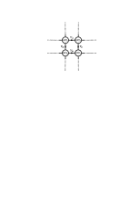
where summation over is understood. In order to simulate the effects of the two extra dimensions in a 4D model, we assume copies of 4D general coordinate invariance (GC), which we denote as , where and . In theory space, each coordinate invariance is represented by one “site” , where any two neighboring sites and with are connected by a link field . Thus, the collection of sites and links forms a two-dimensional transverse lattice (see Fig. 1).
As already pointed out in Ref. [3], this can be simply interpreted as a variation of the Eguchi-Kawai plaquette model for large gauge theories [24].
Each site is equipped with its own metric , which is a function of the 4D coordinates for this site. In order to obtain a lattice version of the derivatives in Eq. (2), we will employ appropriate pullbacks of the coordinates and metrics as defined in Ref. [11]. In this line of thought, a link field can be considered as a pullback function , which maps a vector on the site onto a vector on the site with coordinates . Likewise, to compare the metric on the site with the metric on the site , one can introduce the field , which transforms as a metric tensor under , but is left fixed by . Therefore, is the pullback of the metric on the site to the site .
Assuming equal lattice spacings in both the - and -directions, we can now associate the derivatives in the extra dimensional continuum theory with the nearest neighbor forward difference operators , where for and for . With this definition, we obtain from Eq. (2) a naive transverse lattice formulation of the 6D Einstein–Hilbert action
| (3) | |||||
where and is the fundamental 4D Planck scale, which can, in general, be different from the usual 4D Planck scale . Comparison with Eq. (2) shows that , where is the compactification scale, , and . From Eq. (3) it is evident that we can now equally well drop on all the coordinates the index by making the identification and describe on all sites the positions using only a single universal coordinate system with coordinates .
Following the effective field theory approach advanced in Refs. [11, 12, 13], we can parameterize the link fields in terms of small deviations from as
| (4) |
where behaves in the two-site model defined by and as a Nambu–Goldstone boson, which is eaten to provide the longitudinal component of a massive graviton [11]. In Eq. (4), the Nambu–Goldstone bosons have been rewritten in terms of vector fields and scalars , where the provide the longitudinal components of the massive gravitons. In fact, transforming to the stationary (or unitary) gauge , we observe that the “hopping” terms in Eq. (3) produce graviton mass terms of the Fierz–Pauli type [25]. By analogy with the Eguchi–Kawai model, the model with two discrete gravitational extra dimensions will therefore lead to a multi-graviton theory, containing one zero-mode graviton and a phonon-like spectrum of massive gravitons with masses of order , which simulates in the IR a linear tower of KK excitations.
Now, let us consider small fluctuations of the metrics around Minkowski space and express the gravitons as , where we have introduced the index with and where we have suppressed for simplicity the Lorentz indices. Similarly, we write the scalar modes of the Nambu–Goldstone bosons as , where () if the vector points in the () direction. Inserting Eq. (4) into Eq. (3) and transforming to momentum space, we observe that the action contains a part, which takes in the limit a form of the type
| (5) | |||||
where we have omitted terms involving the transverse spin-1 modes and higher-order terms in the spin-2 excitations. After going to canonical normalization, and , we find from the term in Eq. (5), when evaluated for the lowest lying modes, the strong coupling scale
| (6) |
which is similar to the corresponding value in a single discrete extra dimension. Now, in order to avoid effects that are non-local in theory space [12, 13], the inverse lattice spacing must always be smaller than the maximal short-distance cutoff . Assuming a compactification scale of the order of and , we thus obtain a cutoff , which is by many orders of magnitude smaller than . From a field theory point of view, it would therefore be necessary to provide an understanding of the hierarchy , when the lattice spacing is dynamically generated in a possible UV completion of the theory of massive gravitons.
This hierarchy will be even more enhanced in strong gravitational fields, where the higher-order terms omitted in Eq. (5) can no longer be neglected. Generally, for a macroscopic body with mass , the cutoff gets modified as [11]. Currently, the most precise Cavendish-like tests of Newton’s law use test masses of the order (see, e.g., Ref. [26]). If we are only interested in local theory space models of gravity that admit meaningful predictions in such laboratory experiments, then the inverse lattice spacing must be even smaller than a cutoff . This suggests to consider theory space formulations of large extra dimensions which naturally generate small inverse lattice spacings. Going to the extreme limit where the inverse lattice spacing becomes as small as a few eV, such models would have the additional benefit that the structure of theory space becomes potentially accessible in low-energy experiments via neutrino oscillations, when a right-handed neutrino is propagating in the latticized bulk.
Note that, to prevent the SM from getting strongly coupled at , we would require a perturbative description of the gravitons above this scale. In absence of such an UV completion for gravity, however, we shall in the next section analyze instead a deconstructed gauge theory, which provides an UV completion for the theory of massive gauge bosons. This has the advantage that one can readily formulate an explicit mechanism which produces sub-mm lattice spacings from energy scales above the lattice cutoff, while ensuring that the dynamics of the SM fermions always remains perturbatively sensible.
3 Deconstructed on a disk
In this section, we will study the deconstruction of a gauge theory in a non-gravitational extra dimension compactified on the boundary of a two-dimensional disk. This theory space has been analyzed in the context of supersymmetry breaking [7] and the doublet-triplet splitting problem [27]. Various properties of supersymmetric deconstructed models have also been studied in Ref. [28]. On the boundary of the disk, sub-mm lattice spacings can be generated from a hierarchy between the masses of the link fields. The resulting coarse latticization is experienced by a right-handed neutrino, which propagates on the boundary of the disk and mixes with the SM neutrinos located in the center. The deconstructed acts on the SM fermions as a gauged symmetry that is broken at the TeV scale.
3.1 Gauge sector
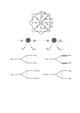
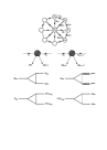
Consider the deconstruction of a gauge theory, which is defined on the boundary of a two-dimensional disk. Our deconstructed theory is described in four dimensions by a product gauge group, where each gauge group corresponds to a site in theory space. The sites are connected by scalar link variables and , each of which carries under exactly two neighboring gauge groups and the charges and transforms trivially under all the other gauge groups. Specifically, for , a link is charged as under the product group , while the link carries the charges . Thus, the sub-graph defined by the link fields has the geometry of a latticized circle. Each link () carries the charges , which leads to a “non-local” theory space, since any two sites are connected through at most two links. The theory space of this model is conveniently represented by the “moose” [29] or “quiver” [30] diagram in Fig. 2.
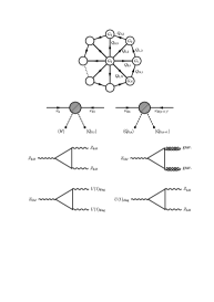
The gauge group corresponds to the center of the disk, while the other gauge groups define the sites on the boundary and are connected by the “boundary links” . The “radial links” connect the center to the sites on the boundary. We wish to reiterate that, in contrast to the previous section, 4D gravity is simply added to the 4D model, i.e., our deconstructed extra-dimensional manifold is non-gravitational.
It is useful to consider the global symmetry which corresponds to a rotation of the disk and acts on the link fields by
| (7) |
where . Using the gauge degrees of freedom, we can always establish an equivalence relation , for , which “identifies” the links on the boundary. Now, for the lattice gauge field “living” on the disk, the holonomy around each plaquette in Fig. 2 is trivial in the lowest energy state. As a consequence, the Wilson lines will break the symmetry down to , where is the diagonal subgroup of and can be taken as a diagonal product (linear combination) of a gauge transformation and the global symmetry [27].
Initially, the scalar sector possesses a global symmetry, which is broken by the gauge couplings, such that only a subgroup is preserved as the gauge symmetry of the model. Wilson line breaking of the global symmetry leads to Nambu–Goldstone boson fields. At the same time, the Wilson lines break also generators of the gauge symmetry, which produces massive spin-1 vector states by eating of the Nambu–Goldstone boson fields via the Higgs mechanism. Thus, we are left with classically massless Nambu–Goldstone bosons in the low-energy theory, which can, however, acquire a mass at the quantum level, since the large global symmetry is explicitly violated in the gauge sector.
The masses of the gauge bosons receive a contribution generated via the Higgs mechanism from the kinetic terms of the link fields , where for is the covariant derivative, in which and denote the gauge coupling and the gauge boson of the group . In the basis , the gauge boson mass squared matrix , which results from these terms after spontaneous symmetry breaking (SSB), is therefore
| (8) |
where we have assumed, for simplicity, universal gauge couplings , while and denote the universal VEV’s and , of the radial and the boundary link fields, respectively. After diagonalization of the mass squared matrix in Eq. (8), we arrive at the gauge boson mass spectrum
| (9) |
where . We observe that this spectrum contains a zero mode, which would correspond to an unbroken (this symmetry will be broken later, when we introduce fermions). In Eq. (9), the tower of mass squares , where , reproduces for a spectrum of KK modes of the order , which has been shifted to higher values by an additional universal contribution of the order provided by the radial links. One gauge boson with mass decouples at low energies for . Thus, in this limit, the theory of massive gauge bosons becomes an effective description of a latticized flat fifth dimension with an inverse lattice spacing (generated by the boundary links) and one lattice scalar (represented by the radial links), which acquires a VEV in the 5D bulk. In the process, the link fields break the total product gauge group down to the diagonal subgroup , which can be further broken by suitable scalar site variables in the center that acquire a VEV at the TeV scale and will thus correspondingly modify the gauge boson spectrum in Eq. (9).
3.2 Large lattice spacings
In order to determine the actual vacuum structure in more detail, let us now consider the scalar potential of the link fields in isolation. The most general gauge invariant renormalizable scalar potential of these fields then reads
| (10) | |||||
where the parameters and have mass dimension +1, while and are dimensionless real parameters of order unity and is a complex-valued order unity coefficient. Note that the potential is invariant under the global symmetry in Eq. (7). From the point of view of usual effective field theories, the dimensionful parameters , and may take any value in the UV desert between and . We will consider here the interesting case where these masses exhibit a hierarchy , i.e., the boundary link fields are much heavier than the radial link fields. To be specific, we assume that the mass is close to the TeV scale, i.e., , while and are of the order the usual breaking scale . Note that an understanding of the smallness of the parameter with respect to may require mechanisms similar to those who give a solution to the -term problem in supersymmetric theories and will not be specifically discussed here.
To explicitly minimize the scalar potential , we shall now make the simplifying assumption that the parameters and in Eq. (10) are real. Actually, in a supersymmetric case, holomorphy of the superpotential sets and one could rotate the phase of into the Yukawa couplings of the neutrinos. Therefore, we argue that our basic results concerning the magnitude of the VEV’s will not be significantly altered, when considering the more general case of complex and . Now, taking and , while , the potential in Eq. (10) has an extremum [35], which is given by and , for , where and are real and equal to
| (11a) | |||||
| (11b) | |||||
i.e., the boundary links and the radial links respectively acquire universal VEV’s. From Eqs. (11) we observe that and become suppressed in the large limit. However, let us now consider the opposite situation, where , i.e., the number of sites is kept moderate or small. In this case, we observe that the choice of mass scales and generates for the boundary link fields a small VEV of the order , while the radial link fields acquire an unsuppressed TeV scale VEV . In other words, the model generates from mass scales in the UV desert of conventional 4D theories an inverse lattice spacing in the IR desert of large extra dimensions. The suppression of due to the hierarchy is similar to the type-II seesaw mechanism [36] and, in fact, the structure of in Eq. (10) can essentially be viewed as a replication of the model in Ref. [37]. It is the replication of gauge groups on the boundary, which allows here to interpret as the sub-mm lattice spacing of a deconstructed large extra dimension.
Note that our mechanism for the generation of sub-mm lattice spacings differs from the model in Ref. [35] essentially in the choice of the dimensionful parameters , , and . In Ref. [35], they are of the orders and . Having , however, would be an automatic consequence in a supersymmetric version, where the tri-linear plaquette terms in Eq. (10) can emerge from the -terms of the superpotential.
3.3 Inclusion of fermions
In our model, we will first extend the three generations of SM fermions by three fermions , , and , which are singlets under the SM gauge group . Then, the three fermion generations are put on the center of the disk by assuming that they carry nonzero charges, but are singlets under the other gauge groups . Note that the addition of matter fields as site variables on the center leaves the symmetry in Eq. (7) unbroken. We suppose that the leptons and ( is the generation index) are charged under as and , respectively, while the quark doublets carry a charge , and the isosinglets , and are given the charges . The SM singlets , , and , carry the charges , , and , respectively. Since the charges of the SM quarks and leptons are identical with their quantum numbers, it is easily seen that the model will be free from axial-vector [31] and gauge-gravitational [32] anomalies. Notice that this is slightly different from the usual way of gauging , where three right-handed SM singlet neutrinos carry a charge [33]. With our charge assignment, however, the Yukawa couplings of the active neutrinos to the fields are suppressed by many powers of and are thus negligible. Suitable SM singlet scalar fields with nonzero charges can then allow renormalizable Yukawa couplings and break the symmetry around the TeV scale. (For a recent detailed analysis of breaking at the TeV scale see, e.g., Ref. [34].) The fields , which were only introduced for the purpose of anomaly cancellation, will then decouple below a TeV.
Next, we include a SM singlet fermion, which appears with respect to the SM interactions as a right-handed neutrino propagating on the boundary of the disk. In the deconstructed space, the bulk fermion is represented by right-handed neutrinos , which are put as site variables on the boundary of the disk. Here, has a charge under the group , but is a singlet under the other gauge groups . In the Weyl basis, we can decompose each field as , where and are two-component Weyl spinors. The mass terms of the neutrinos will be discussed in the next section.
4 Neutrino masses
In this section, we will analyze the kinetic term of the latticized right-handed neutrino and its mixing with the SM neutrinos. Unwanted higher-dimension operators can be eliminated by refining the triangulation of the disk.
4.1 Latticized right-handed neutrino
The deconstructed model presented so far describes a non-local theory space where any two sites are connected by at most two links. This is in contrast to the continuum theory for neutrinos in large extra dimensions [17, 18], where a local interaction of a massless right-handed neutrino in the bulk leads to a suppressed coupling to the active neutrinos. Moreover, the model is in its present form vector-like and allows unprotected Dirac masses . However, if we treat the latticized right-handed neutrino as a massless Wilson fermion [38] propagating on the boundary of the disk, which has lattice spacings in the sub-mm range, we can have only small Dirac masses , where is the inverse lattice spacing. In order to remedy this problem and make contact with the 5D continuum theory in Refs. [17, 18], we introduce for each site on the boundary of the disk a pair of scalars and (), which are singlets, and assume a discrete symmetry ( is an appropriate integer) acting on the fields as
| (12) |
where and runs over all three generations. Note that the left- and right-handed SM fermions carry opposite charges under the symmetry, and hence, the Yukawa couplings of the quarks and charged leptons will remain unsuppressed. Furthermore, we note in Eq. (12) that the potential in Eq. (10) remains invariant under the symmetry. In Appendix A, we show that by adding extra fermions on the boundary the symmetry can be promoted to a discrete gauge symmetry, which would be protected from quantum gravity corrections [39, 40]. It turns out that in the effective theory (ignoring the enlarged gauge symmetry at high energies) all dangerous triangle diagrams would add up to zero. It is interesting to note here, that the SM possesses an anomaly-free symmetry which can ensure nucleon stability for new physics scales as low as [41].
In the deconstructed theory, the action for neutrino masses which includes all renormalizable interactions with Yukawa couplings and the most general invariant dimension-five operators consistent with the discrete symmetry, can now be written as
| (13) |
in which the different parts are given by
| (14a) | |||||
| (14b) | |||||
| (14c) | |||||
where contracts the indices, while and are (complex) dimensionless Yukawa couplings. The non-renormalizable operators and are generated at the string or “fundamental” scale , where a value as low as could be understood in M-theory [42]. In Eq. (14a), let us assume that the acquire a universal VEV , which is equal to the inverse lattice spacing defined by the universal VEV’s of the boundary links in Eq. (11a). We will comment on a possible origin of the order of this mass scale for the VEV’s of the later on. With the identification , the action in Eq. (14a) takes the form of a Wilson-modified latticized 5D kinetic term that describes the propagation of the right-handed neutrino on the boundary of the disk, which is interpreted as a fifth dimension. The fields and in Eq. (14a) are determined by and only up to a discrete “gauge transformation” reflecting the topology of the disk. The symmetry is associated with the existence of non-trivial or twisted field configurations [43] for the latticized right-handed neutrino, which are characterized by distinct spectra in the low-energy theory. In Eq. (14a), we define and , where “” distinguishes between twisted () and untwisted () fields. The effects of twisted field configurations in deconstruction have been extensively discussed in Ref. [44].
Upon using the mechanism in Sec. 3 for generating small inverse lattice spacings , the latticized 5D kinetic term leads then to an effective action for KK modes
| (15) |
In the basis spanned by and , the action in Eq. (15) defines a Dirac mass squared matrix , which explicitly reads
where and the blank entries are all zero. The squared masses of the fermions are found to be the eigenvalues of the matrix . Thus, we obtain for twisted and untwisted fields the mass spectra
| (16) |
where and . We hence observe that reproduces in the IR for and always a tower of KK excitations with masses, which becomes for large indistinguishable from the lightest KK modes of a right-handed bulk neutrino in sub-mm sized continuum extra dimensions. Note in Eq. (16), that a zero mode is absent for twisted fields.
In the above discussion, we require that the acquire the small VEV to allow the interpretation of as the Wilson action for a massless right-handed neutrino. This energy scale has been generated for the VEV’s of the boundary links by the mechanism in Sec. 3. Since the potential for the and is qualitatively similar to the potential of the link fields in Eq. (10), a variation of this mechanism can also produce the right energy scale for , when and take the rôles of the boundary and radial links, respectively. For this purpose, we suppose that the have masses around the TeV scale , whereas the have masses of the order the Planck scale . Additionally, we take in the renormalizable -invariant interactions the dimensionful couplings to be . By the same arguments as in Sec. 3, we find that the can acquire a VEV in the range , which is of the order the inverse lattice spacing in Eq. (11a).
4.2 Non-renormalizable terms
The interaction of the active neutrinos with the right-handed neutrinos on the boundary of the disk is introduced by in Eq. (14b). In theory space, we identify the dimension-five term [45, 46] in with a Wilson line type effective operator, which connects the active neutrinos (in the center of the disk) with (on the boundary) via the link (see Fig. 3).
 |
 |
|
| (a) | (b) |
Let us now go to the basis where in Eq. (15) is on diagonal form and consider the lowest lying mass eigenstate belonging to . After setting to its VEV , the Wilson line type operator generates an effective Yukawa interaction , which is suppressed by a factor with respect to the electroweak scale. For a string scale and small we thus obtain Dirac mass terms , with Dirac masses .
It is instructive to compare the effective Yukawa interaction generated by with the 5D ADD scenario. Here, a right-handed bulk neutrino couples to the active neutrinos on the SM brane through a local interaction [17, 18]
| (17) |
where is the coordinate along the fifth dimension compactified on a circle with circumference , the coefficients are dimensionless Yukawa couplings, and the SM lepton doublets as well as the Higgs doublet are 4D fields trapped at on the SM brane. Note that while in has mass dimension 3/2, the 5D fermion in has mass dimension 2. After expanding in KK modes as and using the relation , it is seen that the interaction in Eq. (17) gives rise to a Dirac type coupling between the active neutrinos and the zero mode , which is suppressed. Since , we thus find that, in the limit of coarse latticizations , the couplings between the active and the right-handed neutrinos generated by and become suppressed by factors of similar orders . However, despite this numerical coincidence, the two models differ in an interesting way: while the smallness of the Dirac type coupling in emerges from a volume suppression factor (i.e., from the large number of KK modes below ), the small Dirac mass generated by is rather a result of the separation between the site where the SM fermions are located and the boundary of the disk as compared to the length scale .
The dimension-five operators contained in in Eq. (14c) give for rise to Dirac mass terms between and that are of the order (see Fig. 3). However, since is the only right-handed neutrino which couples “directly” (at the non-renormalizable level) to the active neutrinos, we may treat the terms in as subleading corrections to , which gives Dirac masses of the order , and ignore them in the following discussion. Let us now, instead, consider a more attractive possibility to suppress the unwanted non-renormalizable terms of the type shown in Fig. 3(b) by making only use of the plaquette-structure of the model. For this purpose, we will assume that the non-local theory space introduced in Sec. 3 is actually part of a larger “spider web theory space” [7] as shown in Fig. 4.
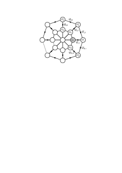
This theory space is obtained from the disk in Fig. 2 by adding extra gauge groups (), which gives the total gauge group . Each pair of factors and is connected by a link field which is charged under as and is a singlet under the other gauge groups. Two neighboring groups and , where , are connected by a boundary link field , that is charged as under and transforms trivially under the other gauge groups.
In analogy with Sec. 3, we suppose that the latticized right-handed neutrino propagates in Fig. 4 on the outer circle defined by the links . Contrary to the previous non-local theory space example, however, the SM fermions are now placed on the site associated with on the inner circle (see Fig. 4). The charge assignment of the SM fermions is similar to that in Sec. 3 with replaced by . Next, we suppose that the boundary link fields on the outer circle have a common mass of the order of an intermediate scale and positive mass squares. The remaining link fields , , and , on the other hand, are supposed to have masses of the order and negative mass squares. By the same arguments as in Sec. 3, we then find that the corresponding scalar potential is extremized for VEV’s , while all other link fields have VEV’s of the order . The separations of the sites on the outer circle are therefore in the sub-mm range, whereas the inverse lattice spacings between all other neighboring sites are of the order . As a result, the active neutrinos couple to the latticized neutrino on the outer circle via an analog of the operator in Eq. (14b), where only has been replaced by . More importantly, the “dangerous” dimension-five operators of the type shown in Fig. 3 (b) are now replaced by dimension-six operators as . As a consequence of the plaquette-structure near the boundary of the spider web theory space, the unwanted higher-dimension operators are suppressed by an extra factor and become therefore irrelevant. We thus see, that the model in Sec. 4.1 is completely reproduced for a fundamental scale , but now without the unwanted higher-dimension terms of the sort given in Eq. (14c).
Up to now, we have been considering the generation of Dirac neutrino masses in a model, where is preserved by the link fields. In order to understand recent solar [47], atmospheric [48], reactor [49], and accelerator [50] neutrino data we assume – contrary to the usual type-I seesaw mechanism [51] – that is broken at the TeV scale. One possibility is here provided by versions of the Babu–Zee model [52], which can be easily implemented in our model to generate radiatively Majorana neutrino masses locally on the site where the SM fermions are located. However, in what follows, we will not further specify the detailed mechanism which generates the Majorana masses of the usual neutrinos. Instead, we will always assume the presence of suitable Majorana mass terms and concentrate in the deconstructed model on the mixing of the SM neutrinos with the KK modes that is introduced by the Dirac neutrino masses.
5 Mixing with Kaluza–Klein modes
In this section, we will consider the neutrino mass and mixing terms of our model by specializing to the simplifying case of only one single active neutrino coupling to the latticized right-handed neutrino, which we treat as a Wilson fermion. From the action in Eq. (13), we thus obtain in this case after SSB for the relevant neutrino mass and mixing terms the action density
| (18) |
where the small inverse lattice spacing has been generated by the mechanism in Sec. 3 and the parameter describes a twisted/untwisted right-handed neutrino. In Eq. (18), the Dirac mass type coupling arises from the higher-dimension operator shown in Fig. 3 (a) (or the analogous term in the extension to spider web theory space with replaced by , see Sec. 4), while the Majorana mass has some other origin and may, e.g., emerge from a radiative mechanism as mentioned in Sec. 4. For convenience, we have chosen for the second term in Eq. (18) a normalization factor , which is related to the volume suppression factor in the corresponding 5D continuum theory.
The action density in Eq. (18) translates into a neutrino mass matrix from which we determine by diagonalization the neutrino mass and mixing parameters for the different cases odd/even and twisted/untwisted. Since , it is useful to define the quantity as an expansion parameter in perturbation theory and diagonalize the matrix in several steps. First, we bring the latticized fermion kinetic term in Eq. (18) on (approximately) diagonal form by applying a transformation with a suitable unitary matrix . The mixing matrices for the different possible cases are explicitly given in Appendix B. For definiteness, let us consider the case and even, the other cases follow then in similar ways. Transforming to momentum space with respect to the latticized dimension defines a new basis , in which the resulting mass squared matrix reads
| (19) |
where the blank entries in this matrix are all zero. The nonzero elements are given by
| (20) |
for and
| (21) |
for . In Eq. (19), the masses and and are
| (22) |
for . The coefficients show the characteristic doubling of KK modes of a phonon-like spectrum, since they satisfy for . In Eq. (19), note that the KK states exhibit no Yukawa interaction with the active neutrino , and hence, decouple completely from the SM interactions. Next, we apply to the basis a sequence of rotations by defining the orthogonal states
| (23) |
for . In Eq. (23), we have and . Crudely, this corresponds to “rotating away” in Eq. (19) half of the interactions , which reduces the degeneracy of the problem from three-fold to two-fold. In the new basis, the mass squared matrix is given by
| (24) |
where
| (25) |
for . Here , , , and are the same as in Eqs. (20) and (22). In the continuum limit, we expect for large to recover some relevant characteristics of a continuous large extra dimension. In order to match onto the 5D continuum theory, we will compare our model with the one given in Ref. [19]. Since in this model Majorana masses are absent, we assume in Eq. (24) that , which implies that . Furthermore, the matrix elements are small in comparison with the quantities and can therefore be neglected when calculating to lowest order. This means that the states spanning in Eq. (24) the top-left submatrix with entries () on the diagonal, decouple from . Consequently, we end up with just one KK tower of states , which span the last rows and columns of in Eq. (24). The remaining entries in become for asymptotically equal to
| (26) |
where we have used the fact that . We will match our model onto the 5D continuum theory by setting , where is some Yukawa coupling in the ADD scenario. With this identification, our model reproduces for the case odd and untwisted (see Table 1) in the IR exactly the effective neutrino mass squared matrix of the 5D continuum theory for neutrino oscillations in extra dimensions as discussed in Ref. [19].
| even | |||||
|---|---|---|---|---|---|
| odd | |||||
| even | |||||
| odd |
Next, we will diagonalize by using two-fold degenerate Rayleigh–Schrödinger perturbation theory. We start by rewriting the mass squared matrix as , where is a diagonal matrix, is the perturbation matrix, and is the small expansion parameter. In order for perturbation theory to be valid, we require that for , where denotes the zeroth order eigenvector, the corresponding eigenvalue, and and are the degeneracy indices. This means that we will require that
| (27) |
From these relations we note that perturbation theory will not be valid for arbitrarily large , since the denominator becomes singular at some point when . For the other cases, , odd and , odd/even, one obtains essentially the same constraints. Now, we apply perturbation theory to this problem and obtain the matrix that diagonalizes as a result. We denote this matrix by , where denotes the th order in perturbation theory. Thus, the mixing matrix which relates the original basis to the mass eigenstate basis via is given by
| (28) |
where are the rotation matrices associated with the state redefinitions in Eq. (23), and , as stated above, is the matrix of eigenvectors of calculated to some order in perturbation theory. The first row is what is of interest to us, since it gives the relevant mixing angles of with the bulk modes. It will be entirely determined by . Thus, to lowest order in perturbation theory, we find
| (29) |
which is an orthogonal matrix, where
| (30) |
for and the elements denoted by are not relevant in the following discussion. Note that one can diagonalize in other ways then the one described above. For example, one could have applied four-fold degenerate perturbation theory directly to the matrix . One can show that this gives the same result for the final neutrino oscillation probabilities. However, reducing the degeneracy makes the problem much easier to handle.
6 Neutrino oscillations
Global analyses have well established that the standard active three-flavor neutrino oscillations with mass squared differences of the orders of magnitude and are in excellent agreement with neutrino oscillation data (see, e.g., Ref. [53]). However, the KK modes of the latticized right-handed neutrino could provide a sizable subdominant component in solar and atmospheric neutrino oscillations, and thus, lead to new anomalies, which are in reach of more precise ongoing or future neutrino oscillation experiments. In this section, we will derive the corresponding neutrino oscillation formulas for our deconstructed model. These will only be valid in the regime where the mixing parameters satisfy the constraints in Eq. (27). For phenomenologically allowed values of the physical parameters, this means that the formulas below will in general be valid for a low or moderate number of sites, .
In order to describe the neutrino oscillations in our model, we can write the flavor eigenstates as a linear combination of the mass eigenstates using the mixing matrix in Eq. (29). We find that
| (31) |
Here denote a flavor eigenstate for some flavor and , , and denote the mass eigenstates. We have also introduced a normalization constant , which follows from the condition . Thus, we find from Eq. (31) that
| (32) |
Next, in the transition survival probability , the time-evolved state is given by
| (33) |
where the phases and the mass-squared eigenvalues equal [cf. Eq. (16)]
| (34) |
in which is the neutrino energy. Using Eqs. (31) and (33) gives for the case and even
| (35) |
For the other cases one finds the transition probability expressions in similar ways, first starting by applying the matrix for the case one considers and then by using a set of rotations similar to the ones given by Eq. (23). Next, one applies perturbation theory and finds the mixing matrix from which the transition survival probability expressions follows. Thus, for the case and odd we have
| (36) |
where
Similarly, for and even we find
| (37) |
where
and is the same as in Eq. (36). Note the presence of a zero mode in the phase . Finally, for and odd we find
| (38) |
where is the same as in Eq. (37). For the cases , and are given by Eq. (30) and the phases are given by Eq. (34), whereas for the cases we have
| (39) |
In this case, the phases are given by Eq. (34), but with the masses [cf. Eq. (16)]
| (40) |
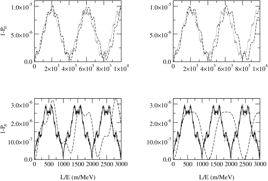
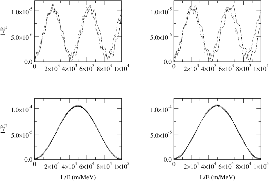
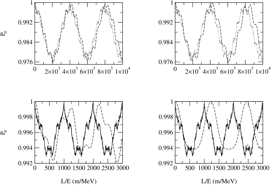
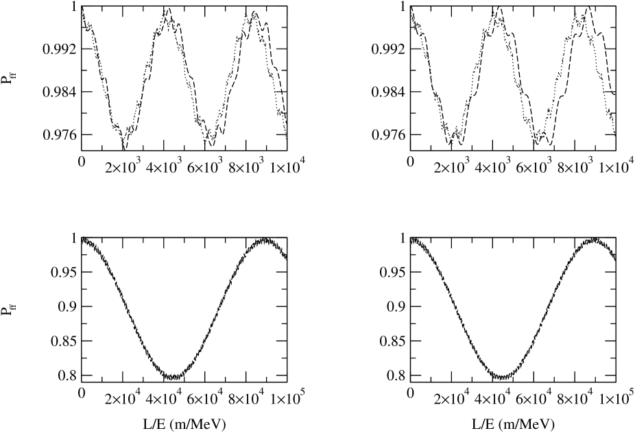
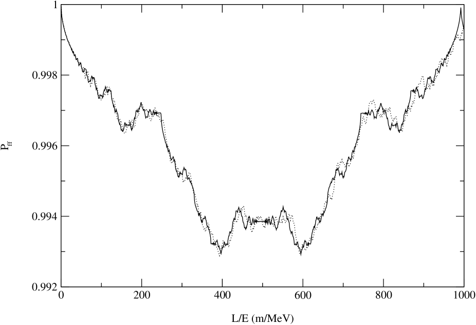
In Figs. 5–8, we have illustrated the different neutrino transition survival probabilities in vacuum as functions of for the different cases and odd/even for some specific choices of . In Figs. 5 and 6, we have given the transition probabilities from Eqs. (35)–(38), where for presentation purposes, we have chosen on the ordinate. From the validity requirements in Eq. (27) we know that Rayleigh–Schrödinger perturbation theory will break down at some point. In Figs. 7 and 8, we have therefore presented the curves from numerical calculations. Nevertheless, at least qualitatively, the neutrino transition survival probabilities show similar patterns for the analytical and the numerical calculations.
In what follows, our choice of parameters would correspond in the ADD scenario to a 4D Planck scale , a SM Higgs doublet VEV , a Yukawa coupling between the active and the bulk neutrinos, and a compactification radius of . In Figs. 5 and 6, the associated fundamental scale would be , which gives . In Figs. 7 and 8, the corresponding fundamental scale would be , which gives . We have distinguished the cases and . In Figs. 6 and 8, we have set , whereas in the other figures, we have set . We have also made a comparison for the cases with the corresponding survival probability in the case of a continuous large extra dimension.
The qualitative behavior of the curves can be understood by looking at the expressions for the survival probabilities, i.e., Eqs. (35)–(38). From these expressions we observe that the dominant effect will be given by the lowest lying modes. For practical purposes one can then average over the higher modes, which means that the essential behavior will be determined by only a few low modes. Let us first consider the case . We obtain for and even the survival probability, when only the first mode is non-averaged, as , where the amplitude and the frequency are given by and , respectively. For the other cases we obtain similar results.
First, we observe that the frequencies are proportional to , i.e., a smaller radius gives faster oscillations. We also note that the frequencies differ for the cases and . This is due to the different mass eigenvalues that appear in the phases. Thus, we have for the case , when only the first mode is non-averaged, that the frequency is proportional to . However, for the case the frequency is proportional to , which is roughly four times larger than for the case . This can be directly seen in Fig. 5. The figures also show a dependency of the frequency on . This is because the frequency in for example the case is proportional to . This function grows rapidly for small and converges quickly to a fixed value, . A similar relation holds for the case . This effect is best visible when .
Second, the amplitude is proportional to so that a change of these parameters significantly affects the amplitude. This can be seen by comparing for example Figs. 5 and 7. There is also a difference in amplitude between the cases and . For the case the amplitude is proportional to , where for is given in Eq. (30). However, for the case the amplitude is proportional to where for is given in Eq. (39). Since the amplitude will be larger for .
Note that the case and differs in a significant way from the other cases. The aperiodic behavior of this curve is due to the large interference effect between the two lowest modes, which together give the dominating behavior. This effect can be seen in the relation between the factors and . As we increase , the effect of will be suppressed in comparison with , so that we for large obtain a sinusoidal-like behavior. For the case and there is no large interference effect between low-lying modes, since the sum in this case only includes one term. For the case the corresponding ratio which gives the interference effect is . This ratio is smaller than the ratio for the case . Thus, for we do not observe any significant distortion of the periodicity.
Let us now consider the effect of a non-zero . For we note that there will be an effect provided that is large enough. If , the frequency will be determined by . However, for the case we have considered, we have chosen and , which means that the frequency will mainly be determined by . Thus, for the case there will be no drastic changes, which can be seen when comparing the upper rows of Figs. 5 and 6. For , on the other hand, there will be a significant effect from . This is obvious from Eqs. (37) and (38), where the survival probability expressions contain a term , in which is approximately given by . If is sufficiently small, then this term will be the dominating term. Thus, the survival probability will be proportional to . This is the case in the lower row of Fig. 6. Note that this effect is due to the presence of a zero mode, which is absent for .
If is increased, then the curves obtains a more jagged shape because of the interference of a large number of KK modes with different frequencies [18]. However, essential properties such as the amplitude and the frequency quickly stabilizes. Finally, we observe in Figs. 5 and 7 that the case reproduces the continuum case [19, 21] as expected.
We have seen that one could, at least in principle, probe as well as the number of lattice sites through neutrino oscillation experiments. For low the best probe of is through the frequency.
7 Summary and Conclusions
In this paper, we have considered a model for neutrino oscillations in a deconstructed gauge theory defined on the boundary of a two-dimensional disk. If the masses of the link fields connecting the center with the boundary are of the order (), while the link fields on the boundary have masses of the order (), then the model generates sub-mm lattice spacings between the sites on the boundary. This allows to obtain dynamically a non-gravitational large extra dimension with only a few sites. Here, we have motivated the general significance of large (sub-mm) lattice spacings by reviewing the strong coupling behavior of gravity in local theory spaces for the example of two discrete gravitational extra dimensions.
We have analyzed the mass and mixing properties of a latticized right-handed neutrino, which propagates on the boundary of the disk and may be twisted or untwisted. A discrete cyclic symmetry, which can be gauged, allows to treat the latticized right-handed neutrino as a Wilson fermion with vanishing bare mass. At the same time, the cyclic symmetry also introduces in the non-local theory space a local Yukawa interaction between the active SM neutrinos and the latticized right-handed neutrino. As a consequence, the model simulates key features of the 5D continuum theory for neutrinos in the ADD scenario.
We have studied the neutrino oscillation effects of the latticized right-handed neutrino in terms of the survival probability of a single active flavor for the cases of a twisted (untwisted) lattice fermion and an even (odd) number of sites on the boundary. By taking the continuum limit, we could exactly reproduce known oscillation patterns of existing 5D continuum theory models. The most direct probe of our model parameters is through the frequency of . For example, if the number of lattice sites is small, then can exhibit a strongly aperiodic behavior for odd . Possible “odd-even artifacts”, however, quickly disappear when becomes large. Generally, twisted and untwisted field configurations can be distinguished through the different associated frequencies of , which is for an untwisted neutrino roughly four times larger than for a twisted one. The presence or absence of an active Majorana neutrino mass also affects the oscillation patterns of twisted and untwisted neutrinos in qualitatively different ways. Generally, it should be noted, however, that in more elaborate models one would have to include three flavors (as well as matter effects). It could also be necessary to take into account additional large extra dimensions. Therefore, the results obtained from our model should be viewed as comparatively qualitative.
The neutrino oscillation effects that are introduced by the KK neutrinos could, in principle, be observed in present and future precision neutrino oscillation experiments, such as for example KamLAND [49], Borexino [54], or the proposed Double-CHOOZ [55] experiment. Borexino would be capable to search for new solar neutrino oscillation effects in an energy range not covered by Super-Kamiokande or SNO [47]. Our model could be tested at short baselines by (future) (or ) disappearance experiments with sensitivities for mixing angles between the active and the KK-neutrinos. Here, it could prove useful to employ also two-reactor-two-detector-setups [56], where one may perform measurements practically free from the typical systematic uncertainties in the reactor neutrino fluxes. More generally, one can consider any experiment, which probes the effect of sterile neutrinos, provided that one can identify the masses and mixings properly.
The non-zero mixing between the SM Higgs and the scalar link and site variables will lead to invisible decays (if these processes are kinematically allowed), which can be checked at the LHC or a future linear collider.
It is clear, that standard Big Bang nucleosynthesis [57] will be affected by the presence of the KK neutrinos. However, the bounds from measurements of the abundance can be alleviated by assuming a primordial lepton asymmetry [58] or with low reheating temperature [59]. The constraints on the effective number of neutrino species from large scale structure data in conjunction with cosmic microwave background measurements [60] may also be evaded by such a lepton asymmetry [61]. Also note that, in this paper, we have assumed the same constraints that apply to continuous large gravitational extra dimensions, but it has been argued [2] that several of the standard constraints could be relaxed for non-gravitational deconstructed dimensions.
Acknowledgments
We would like to thank K.S. Babu, T. Enkhbat, I. Gogoladze, and M.D. Schwartz for useful comments and discussions. One of us (G.S.) would like to thank the division of mathematical physics at the Royal Institute of Technology (KTH), Stockholm, Sweden, for the warm hospitality during the stays at KTH, where part of this work was developed. This work was supported by the Swedish Research Council (Vetenskapsrådet), Contract Nos. 621-2001-1611, 621-2002-3577 (T.O.), the Göran Gustafsson Foundation (T.H. and T.O.), the Magnus Bergvall Foundation (T.O. and G.S.), and the U.S. Department of Energy under Grant Nos. DE-FG02-04ER46140 and DE-FG02-04ER41306 (G.S.).
Appendix A Cancellation of anomalies
The discrete symmetry in Eq. (12) introduces on each site on the boundary of the disk a parity-asymmetry between and . The model in Sec. 4 for the Wilson fermion is therefore chiral. If we wish to gauge the symmetry, we will have to ensure that the model remains free from chiral anomalies and that all anomalous contributions from triangle diagrams to the three-gauge-boson vertex functions cancel. In the low-energy effective theory, the apparent unbroken gauge symmetry444We neglect here the symmetry breaking introduced by the scalar site variables on the center (see Sec. 3). of the deconstructed model would be and it is only at short distance scales that we become aware of the underlying enlarged gauge symmetry. It is interesting to compare in these two limiting cases the formal cancellation of anomalous diagrams by defining the gauge symmetry (containing the discrete factor) of our model to be either
| (41) |
Implicitly, model (a) becomes equivalent with a non-linear sigma model approximation of the deconstructed model in Sec. 3. Of course, if we are interested in the UV completing linear sigma model description, only the anomalies calculated in model (b) are of relevance.
To work out the anomaly cancellation for models (a) and (b) in Eq. (41), we will denote the , , and charges of a field by , , and , respectively. First, we observe that the fermions located on the center of the disk – i.e., the SM fermions and the fields – satisfy . Thus, the SM fermions and the do not contribute to any anomalies and we can from now on concentrate on the anomalous diagrams involving only the right-handed neutrinos and . Since the and gauge bosons couple equally to and on each site on the boundary, all anomalies which do not involve a coupling vanish automatically. Consider now the triangle diagrams in Fig. 10, which do not have any or gauge bosons at their vertices.
 |
 |
|
| (i) | (ii) |
If we choose in Eq. (12) , then in both models (a) and (b), the cubic anomaly (i) and the gauge-gravitational anomaly (ii) are proportional to
| (42) |
where we have used that and , implying that the anomalies cancel between neighboring sites and vanish when summing over all right-handed neutrino species.
The anomaly cancellations differ substantially between model (a) and (b) when evaluating the triangle diagrams of the type shown in Fig. 11, which have at least one gauge boson at one of their vertices.
 |
 |
|
| (i) | (ii) |
Let us first restrict to model (a). In Fig. 11, the mixed anomaly (i) and the anomaly (ii) are proportional to
| (43) |
where we have used that . Again, the diagrams cancel between neighboring sites and vanish when summing over all sites. In total, we thus find that all divergent triangle diagrams in model (a) formally add up to zero. Let us next consider the corresponding anomalies in model (b). The dangerous mixed and anomalies are obtained from the diagrams in Fig. 11 by replacing in (i) and (ii) the gauge bosons according to . In this case, the diagrams (i) and (ii) in Fig. 11 become divergent and the summation over all sites does not remove the divergences, since the diagrams belonging to different lattice sites have different external legs and are thus inequivalent.
In order to remove the anomalies in model (b), we add on each site of the boundary extra fermions with appropriate quantum numbers. We place on the site corresponding to the gauge group () three additional Dirac spinors, which are written component-wise in the Weyl basis as , , and . The fields , , and carry the charges , , and , respectively, and are singlets under and the other gauge groups . In addition, we assume that the extra fermions carry specific charges. The and charge assignment for all SM singlet fermions is summarized in Table 2.
| field | ||||||||
|---|---|---|---|---|---|---|---|---|
¿From Table 2, we find that the cubic and gauge-gravitational and anomalies still vanish, since the and symmetries satisfy for the extra fermions relations similar to Eq. (42). The mixed anomaly is proportional to
| (44) |
where each bracketed term inside the sum is zero. Therefore, these anomalies cancel on each site. The mixed anomaly is proportional to
| (45) |
where each bracketed expression inside the sum vanishes. Again, all anomalies cancel individually on each lattice site. In total, the symmetry is therefore anomaly-free. In addition, this model is chiral, since the symmetry forbids any bare mass terms for the fermions.
Appendix B Neutrino mixing matrices
In the basis , the total neutrino mass matrix described by the action density in Eq. (18) takes the form
| (46) |
where and denote and matrices respectively, which are explicitly given by
| (47) |
Here, the Majorana-like matrix is defined in the basis , whereas the Dirac-like matrix is spanned by and . In Eq. (46), “0” denotes an matrix with zero entries only. The neutrino masses and mixing angles can be determined from the product , which in this basis explicitly reads
| (48) |
where and the blank entries are zero. Next, we want to diagonalize this matrix. Since , we can define the quantity , which we will use as an expansion parameter in perturbation theory. We will diagonalize the matrix in steps. First, we perform the transformation using the block-diagonal matrix , where denotes a unitary matrix. For and even, the matrix reads
| (49) |
whereas for and odd, we have
| (50) |
Similarly, for and even, we have
| (51) |
and finally, for and odd, we have
| (52) |
In Sec. 5, we consider the case and even. The other cases follow in similar ways. The rotation from the matrix in Eq. (49) has the effect of diagonalizing the “gauge-boson-like” submatrices in Eq. (48) and leads in the new basis to the matrix in Eq. (19), which can then be further diagonalized using perturbation theory as described in Sec. 5.
References
- [1] T. Kaluza, Sitzungsber. Preuss. Akad. Wiss. Berlin (Math. Phys.) K21 (1921) 966; O. Klein, Z. Phys. 37 (1926) 895.
- [2] N. Arkani-Hamed, A.G. Cohen, and H. Georgi, Phys. Rev. Lett. 86 (2001) 4757, hep-th/0104005.
- [3] C.T. Hill, S. Pokorski, and J. Wang, Phys. Rev. D 64 (2001) 105005, hep-th/0104035.
- [4] M.B. Halpern and W. Siegel, Phys. Rev. D 11 (1975) 2967.
- [5] H.C. Cheng, C.T. Hill, S. Pokorski, and J. Wang, Phys. Rev. D 64 (2001) 065007, hep-th/0104179; H.C. Cheng, C.T. Hill, and J. Wang, Phys. Rev. D 64 (2001) 095003, hep-ph/0105323; C. Csaki, G.D. Kribs, and J. Terning, Phys. Rev. D 65 (2002) 015004, hep-ph/0107266; H.C. Cheng, K.T. Matchev, and J. Wang, Phys. Lett. B 521 (2001) 308, hep-ph/0107268; A. Falkowski, C. Grojean, and S. Pokorski, Phys. Lett. B 535 (2002) 258, hep-ph/0203033; H. Abe, T. Kobayashi, N. Maru, and K. Yoshioka, Phys. Rev. D 67 (2003) 045019, hep-ph/0205344; T. Gregoire and J.G. Wacker, hep-ph/0207164; L. Randall, Y. Shadmi, and N. Weiner, J. High Energy Phys. 0301 (2003) 055, hep-th/0208120; N. Maru and K. Yoshioka, Eur. Phys. J. C 31 (2003) 245, hep-ph/0311337; A. Falkowski, C. Grojean, and S. Pokorski, Phys. Lett. B 581 (2004) 236, hep-ph/0310201; Z. Kunszt, A. Nyffeler, and M. Puchwein, JHEP 0403 (2004) 061, hep-ph/0402269.
- [6] W.A. Bardeen and R.B. Pearson, Phys. Rev. D 14 (1976) 547; W.A. Bardeen, R.B. Pearson, and E. Rabinovici, Phys. Rev. D 21 (1980) 1037.
- [7] N. Arkani-Hamed, A.G. Cohen, and H. Georgi, JHEP 0207 (2002) 020, hep-th/0109082.
- [8] C.T. Hill, Phys. Rev. D 67 (2003) 085004, hep-th/0210076; hep-th/0303267.
- [9] K.R.S. Balaji, M. Lindner, and G. Seidl, Phys. Rev. Lett. 91 (2003) 161803, hep-ph/0303245.
- [10] P.Q. Hung, A. Soddu, and N.K. Tran, hep-ph/0410179; P.Q. Hung and N.K. Tran, hep-ph/0410269.
- [11] N. Arkani-Hamed, H. Georgi, and M.D. Schwartz, Annals Phys. 305 (2003) 96, hep-th/0210184.
- [12] N. Arkani-Hamed and M.D. Schwartz, Phys. Rev. D 69 (2004) 104001, hep-th/0302110.
- [13] M.D. Schwartz, Phys. Rev. D 68 (2003) 024029, hep-th/0303114.
- [14] N. Arkani-Hamed, S. Dimopoulos, and G.R. Dvali, Phys. Lett. B 429 (1998) 263, hep-ph/9803315; Phys. Rev. D 59 (1999) 086004, hep-ph/9807344; I. Antoniadis, N. Arkani-Hamed, S. Dimopoulos, and G.R. Dvali, Phys. Lett. B 436 (1998) 257, hep-ph/9804398.
- [15] L. Randall and R. Sundrum, Phys. Rev. Lett. 83 (1999) 3370, hep-ph/9905221; Phys. Rev. Lett. 83 (1999) 4690, hep-th/9906064.
- [16] D. Cremades, L.E. Ibáñez, F. Marchesano, Nucl. Phys. B 643 (2002) 93, hep-th/0205074; C. Kokorelis, Nucl. Phys. B 677 (2004) 115, hep-th/0207234.
- [17] N. Arkani-Hamed, S. Dimopoulos, G.R. Dvali, and J. March-Russell, Phys. Rev. D 65 (2002) 024032, hep-ph/9811448.
- [18] K.R. Dienes, E. Dudas, and T. Gherghetta, Nucl. Phys. B 557 (1999) 25, hep-ph/9811428.
- [19] G.R. Dvali and A.Y. Smirnov, Nucl. Phys. B 563 (1999) 63, hep-ph/9904211.
- [20] R.N. Mohapatra, S. Nandi, and A. Pérez-Lorenzana, Phys. Lett. B 466 (1999) 115, hep-ph/9907520.
- [21] R.N. Mohapatra and A. Pérez-Lorenzana, Nucl. Phys. B 593 (2001) 451, hep-ph/0006278
- [22] G. Moreau, hep-ph/0407177
- [23] T. Han, J.D. Lykken, and R.J. Zhang, Phys. Rev. D 59 (1999) 105006, hep-ph/9811350.
- [24] T. Eguchi and H. Kawai, Phys. Rev. Lett. 48 (1982) 1063.
- [25] M. Fierz and W. Pauli, Proc. Roy. Soc. Lond. A 173 (1939) 211.
- [26] C.D. Hoyle, D.J. Kapner, B.R. Heckel, E.G. Adelberger, J.H. Grundlach, U. Schmidt, and H.E. Swanson, hep-ph/0405262.
- [27] E. Witten, hep-ph/0201018.
- [28] A. Falkowski, H.P. Nilles, M. Olechowski, and S. Pokorski, Phys. Lett. B 566 (2003) 248, hep-th/0212206; E. Dudas, A. Falkowski, and S. Pokorski, Phys. Lett. B 568 (2003) 281, hep-th/0303155.
- [29] H. Georgi, Nucl. Phys. B 266 (1986) 274.
- [30] M.R. Douglas and G. Moore, hep-th/9603167.
- [31] S.L. Adler, Phys. Rev. 177 (1969) 2426; J.S. Bell and R. Jackiw, Nuovo Cimento A 60 (1969) 47; W.A. Bardeen, Phys. Rev. 184 (1969) 1848.
- [32] R. Delbourgo and A. Salam, Phys. Lett. B 40 (1972) 381; T. Eguchi and P.G.O. Freund, Phys. Rev. Lett. 37 (1976) 1251; L. Álvarez-Gaumé and E. Witten, Nucl. Phys. B 234 (1984) 269.
- [33] R.E. Marshak and R.N. Mohapatra, Phys. Lett. B 91 (1980) 222.
- [34] O.C. Anoka, K.S. Babu, and I. Gogoladze, Nucl. Phys. B 687 (2004) 3, hep-ph/0401133.
- [35] F. Bauer, M. Lindner, and G. Seidl, JHEP 0405 (2004) 026, hep-th/0309200.
- [36] R.N. Mohapatra and G. Senjanović, Phys. Rev. Lett. 44 (1980) 912; Phys. Rev. D 23 (1981) 165; J. Schechter and J.W.F. Valle, Phys. Rev. D 22 (1980) 2227; G. Lazarides, Q. Shafi, and C. Wetterich, Nucl. Phys. B 181 (1981) 287.
- [37] E. Ma and U. Sarkar, Phys. Rev. Lett. 80 (1998) 5716, hep-ph/9802445.
- [38] K.G. Wilson, Phys. Rev. D 10 (1974) 2445.
- [39] L.M. Krauss and F. Wilczek, Phys. Rev. Lett. 62 (1989) 1221.
- [40] L.E. Ibanez and G.G. Ross, Phys. Lett. B 260 (1991) 291; Nucl. Phys. B 368 (1992) 3.
- [41] K.S. Babu, I. Gogoladze, and K. Wang, Phys. Lett. B 570 (2003) 32, hep-ph/0306003.
- [42] E. Witten, Nucl. Phys. B 471 (1996) 135, hep-th/9602070.
- [43] C.J. Isham, Proc. R. Soc. Lond. A. 362 (1978) 383; C.J. Isham, Proc. R. Soc. Lond. A. 364 (1978) 591; S.J. Avis and C.J. Isham, Nucl. Phys. B 156 (1979) 441.
- [44] C.T. Hill and A.K. Leibovich, Phys. Rev. D 66 (2002) 016006, hep-ph/0205057.
- [45] S. Weinberg, Phys. Rev. Lett. 43 (1979) 1566.
- [46] F. Wilczek and A. Zee, Phys. Rev. Lett. 43 (1979) 1571.
- [47] SNO Collaboration, Q.R. Ahmad et al., Phys. Rev. Lett. 87 (2001) 071301; SNO Collaboration, Q. R. Ahmad et al., nucl-ex/0309004; Super-Kamiokande Collaboration, S. Fukuda et al., Phys. Lett. B 539 (2002) 179, hep-ex/0205075.
- [48] Super-Kamiokande Collaboration, Y. Fukuda et al., Phys. Rev. Lett. 81 (1998) 1562; Phys. Lett. B 467 (1999) 185.
- [49] KamLAND Collaboration, K. Eguchi et al., Phys. Rev. Lett. 90 (2003) 021802, hep-ex/0212021.
- [50] K2K Collaboration, M.H. Ahn et al., Phys. Rev. Lett. 90 (2003) 041801, hep-ex/0212007.
- [51] P. Minkowski, Phys. Lett. B 67 (1977) 421; T. Yanagida, in Proceedings of the Workshop on the Unified Theory and Baryon Number in the Universe, KEK, Tsukuba, 1979; M. Gell-Mann, P. Ramond, and R. Slansky, in Proceedings of the Workshop on Supergravity, Stony Brook, New York, 1979.
- [52] A. Zee, Nucl. Phys. B 263 (1986) 99; K.S. Babu, Phys. Lett. B 203 (1988) 132; K.S. Babu and C. Macesanu, Phys. Rev. D 67 (2003) 073010, hep-ph/0212058.
- [53] M. Maltoni, T. Schwetz, M. Tórtola, and J.W.F. Valle, New J. Phys. 6 (2004) 122, hep-ph/0405172.
- [54] Borexino Collaboration, G. Alimonti et al., Astropart. Phys. 16 (2002) 205, hep-ex/0012030.
- [55] F. Ardellier et al., hep-ex/0405032; S. Berridge et al., hep-ex/0410081.
- [56] P. Huber, M. Lindner, and T. Schwetz, hep-ph/0411166.
- [57] T.P. Walker, G. Steigman, D.N. Schramm, K.A. Olive, and H.S. Kang, Astrophys. J. 376 (1991) 51.
- [58] R. Foot and R.R. Volkas, Phys. Rev. Lett. 75 (1995) 4350, hep-ph/9508275; R. Foot, M.J. Thomson, and R.R. Volkas, Phys. Rev. D 53 (1996) 5349, hep-ph/9509327; P. Di Bari, Phys. Rev. D 65 (2002) 043509, hep-ph/0108182; Addendum-ibid D 67 (2003) 127301, astro-ph/0302433; K.N. Abazajian, Astropart. Phys. 19 (2003) 303, astro-ph/0205238; for a recent comprehensive review see, M. Cirelli, G. Marandella, A. Strumia, and F. Vissani, hep-ph/0403158.
- [59] G. Gelmini, S. Palomares-Ruiz, and S. Pascoli, Phys. Rev. Lett. 93 (2004) 081302, astro-ph/0403323.
- [60] The 2dFGRS Collaboration, Ø. Elgarøy et al., Phys. Rev. Lett. 89 (2002) 061301, astro-ph/0204152; WMAP Collaboration, D.N. Spergel et al., Astrophys. J. Suppl. 148 (2003) 175, astro-ph/0302209.
- [61] S. Hannestad and G. Raffelt, JCAP 0404 (2004) 008, hep-ph/0312154.