The Use of the Scattering Phase Shift in Resonance Physics

Abstract

The scattering phase shift encodes a good amount of physical information which can be used to study resonances from scattering data. Among others, it can be used to calculate the continuum density of states and the collision time in a resonant process. Whereas the first information can be employed to examine the evolution of unstable states directly from scattering data, the second one serves as a tool to detect resonances and their properties. We demonstrate both methods concentrating in the latter case on ‘exotic’ resonances in $\pi\pi$ and $\pi K$ scattering.

1 The Phase Shift and its Ambiguities

The phase shift $\delta_{l}$ is a convenient variable to parameterize the scattering amplitude as known from many textbooks on quantum mechanics. In principle, the phase shift can be extracted from the differential cross section $d\sigma/d\Omega$ or other observables. To understand a physical problem from a scattering experiment it is often sufficient to know the differential cross section. A good example is a bump in the cross section which signals often a resonance. However, the knowledge of the phase shift (or amplitude) can give us additional information on the dynamics of the scattering process, the properties of occurring resonances etc. We shall discuss two such applications of the phase shift in the subsequent sections. Both have to do with resonances as intermediate states in the scattering process from which $\delta_{l}$ is determined. It is therefore not unimportant to remind the reader of some facts regarding the extraction of the phase shift from experiment. Only if the extraction is unambiguous and clean can we rely on the information stored in the extracted data. The usage of the differential cross section is not enough for this purpose because of several ambiguities encountered in the process. Here we will just mention two of them: the so-called Yang [1] and Minami [2] ambiguities. The first one allows for two different solutions in case that only $S$ and $P$ waves are present (important) in the reaction under consideration. The relation between the two solutions, primed and unprimed, reads: $\delta(S_{31})=\delta^{\prime}(S_{31})$ and $\delta(P_{33})-\delta(P_{31})=\delta^{\prime}(P_{31})-\delta^{\prime}(P_{33})$. The second famous ambiguity is called Minami after its discoverer. It is based as all such ambiguities on the invariance of the differential cross section under a certain transformation. In case of the Minami ambiguity this is $\delta_{j+1/2}\leftrightarrow\delta_{j-1/2}$ where $j$ is the total angular momentum. Hence more specifically one obtains $\delta(S_{1})\leftrightarrow\delta(P_{1})$, $\delta(P_{3})\leftrightarrow\delta(D_{3})$ and $\delta(D_{5})\leftrightarrow\delta(F_{5})$. There are more ambiguities which we will not discuss here. But the point we wish to make is that because of these ambiguities a differential cross section is not sufficient to extract the phase shift and more data such as the polarization observables are necessary [3]. In addition, the extracted phase shifts must pass a number of tests based on basic properties of the $S$-matrix like unitarity, analyticity and crossing symmetry. For instance, in $\pi\pi$ scattering these are gathered in the so-called Roy equations and the $\pi\pi$ phase shift has to satisfy the latter in order to be accepted as an unambiguous physical quantity [4].

This way the experimental phase shifts are indeed trustworthy physical values which we can use to get some insight into the scattering process. In the next section we will give some examples on how these values might be used and processed.

2 Physics from the Phase Shift

Having convinced ourselves that the extraction of the phase shift is reliable, we proceed to discuss two examples of how to use and interpret the derivative of the phase shift $\frac{d\delta_{l}}{dE}$ to obtain physically relevant information on the resonances occurring in the process.

2.1 Continuum Level Density

While calculating correction factors $B$ and $C$ to the equation of states of an ideal gas, namely, $pV=RT[1+B/V+C/V^{2}]$, Beth and Uhlenbeck [5] found that the derivative of the phase shift is proportional to the difference of the density of states (of the outgoing particles) with and without interaction. In case of the $l^{th}$ partial wave we have then,

$$n_{l}(E)-n^{(0)}_{l}(E)=\frac{2l+1}{\pi}\frac{d\delta_{l}(E)}{dE}\,.$$ (1)

This is an interesting result. To appreciate it, let us briefly recall the Fock-Krylov method to study the time evolution of unstable states. It is based on the fact that unstable states cannot be eigenstates to the Hamiltonian and as a result we can expand the resonance states in terms of the energy eigenstates; i.e.

$$|\Psi\rangle=\int dE\,a(E)|E\rangle\,.$$ (2)

With a little bit of algebra we can recast the survival amplitude in a Fourier transformation of the so-called spectral function $\rho_{{}_{\Psi}}=|a(A)|^{2}$ which is the probability density to find the state $|E\rangle$ between $E$ and $E+dE$. This way we obtain the Fock-Krylov celebrated result [6]

$$A_{\Psi}(t)=\int_{E_{th.}}^{\infty}dE\rho_{{}_{\Psi}}(E)e^{-iEt}$$ (3)

used in many investigations on quantum time evolution [7]. Now the probability density and the continuum density of states are related by a constant. As long as there are no interfering resonances $\frac{d\delta}{dE}$ is positive and the above identification works without doubt. The best example is the Lorentzian (Breit-Wigner) spectral density which is very often used in investigations of the decay problem [8]. Indeed, $T=\frac{\Gamma/2}{E_{R}-E-i\Gamma/2}$ gives rise to a phase shift $\delta$ such that $\frac{d\delta}{dE}=\frac{\Gamma/2}{(E_{R}-E)^{2}+\Gamma^{2}/4}$. In case of several resonances the interference pattern can cause the derivative of the phase shift to become negative. Therefore, it is safe to take the first resonance and neglect the subsequent contribution of the higher lying resonances. We can do that if we want to study only the large time behaviour of the time evolution because in this case due to the time-energy duality we need to know only the threshold behaviour of the phase shift. We can parameterize $\rho_{{}_{\Psi}}$ without loss of generality in the form $\rho_{{}_{\Psi}}\propto(E-E_{\rm th.})^{\gamma}$ to account for the threshold. Hence we have

$$\rho_{{}_{\Psi_{l}}}(E)=G(E)(E-E_{\rm th.})^{\gamma(l)}\,.$$ (4)

The form factor has the property $G(E)\to 0$ sufficiently fast as $E\to\infty$ and a complex pole $z_{0}$, i.e. $1/G(z_{0})=0$ such that $\Im m(z_{0})<0$ and $\Re e(z_{0})>0$. This pole represents the resonance at $E_{R}-i\Gamma/2$ and leads to the exponential decay. This generalizes the simple Breit-Wigner form which has the pole but no threshold behaviour. These general properties of the spectral function allow us to compute the survival probability by going to the complex plane. We choose the closed path $C_{\rm R}=C_{\Im}+C_{\Re}+C_{\rm R}^{1/4}$, starting from zero (after change of variables $y=E-E_{th}$) along the real axis ($C_{\Re}$) attaching to it a quarter of a circle with radius ${\rm R}$ ($C_{\rm R}^{1/4}$) in the clockwise direction and completing the path by going upward the imaginary axis up to zero ($C_{\Im}$). In the integral we let ${\rm R}$ go to infinity noting that along $C_{{\rm R}\to\infty}^{1/4}$, the integral is zero. We subtract the contribution along the imaginary axis. This gives

$$A_{\Psi_{l}}(t)=A_{\Psi_{l}}^{\rm E}(t)+A_{\Psi_{l}}^{\rm P}(t)$$ (5)

with

$$A_{\Psi_{l}}^{\rm E}(t)=e^{-iE_{\rm th.}t}\lim_{{\rm R}\to\infty}\oint_{C_{\rm R}}dze^{-izt}z^{\gamma}G(z+E_{\rm th.})=C_{1}\,e^{-iE_{R}t}e^{-\Gamma/2\,t}$$ (6)

by Cauchy’s theorem and

$$A_{\Psi_{l}}^{\rm P}(t) = C_{2}\,e^{-iE_{th.}t}\int_{0}^{\infty}dxe^{-xt}x^{\gamma}G(-ix+E_{\rm th.})$$ (7)

$$\simeq C_{2}\,e^{-iE_{th.}t}G(E_{\rm th.})\Gamma(\gamma+1)\,{1\over t^{\gamma+1}}$$

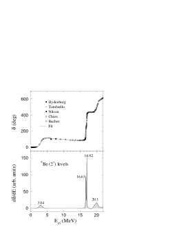
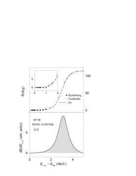
Figure 1: D-wave phase shift (upper half) [9] and its derivative (lower half) in $\alpha$-$\alpha$ elastic scattering as a function of $E_{ex}=E_{c.m.}-E_{{}^{8}{\rm Be}{\rm(groundstate)}}$. The figure on the right displays the region of the first $2^{+}$ level of ${}^{8}{\rm Be}$ in detail. The inset displays the accuracy of our fit near the threshold energy region which is crucial for the large time behaviour of the decay law.

for the integral along $C_{\Im}$, where the approximation is valid for large times $t$. In the above, $\Gamma(x)$ is the Euler’s gamma function and $C_{1}$ is a constant easily calculable in terms of the parameters $E_{R}$, $\Gamma$ and $E_{\rm th.}$ and $C_{2}$ is $(-i)^{\gamma+1}$. Equations (6) and (7) show the general features which we would expect: an exponential decay law followed by inverse power law corrections. The latter is independent of the details of $G(E)$ displaying also the dual nature of time and energy. Our choice of the elastic resonant reaction from which we want to extract the information on the long tail of the decay is dictated by very good data at threshold. We opted for $\alpha+\alpha\to{}^{8}Be(2^{+})\to\alpha+\alpha$ (see Figure 1) [9]. The analysis of this data following the mathematical method outlined above or alternatively by numerical integration reveals that the survival probability behaves as $P_{\Psi}(t)=|A_{\Psi}(t)|^{2}\sim t^{-6.36}$ for large times [10].

Interestingly one can also use the interpretation of $d\delta/dE$ as continuum level density to calculate the density of resonances per unit volume and unit invariant mass in a thermal environment e.g. in heavy ion collisions [11]. This is $\frac{dn}{dM}\propto\int\frac{d^{3}p}{(2\pi)^{3}\pi}\,\frac{d\delta}{dM}\,\frac{1}{\exp{(E_{p}/T)}\pm 1}$ and is proportional to the probability density to form this resonances.

2.2 Time delay

In Figure 1 we can see that all resonances of ${}^{8}Be$ with $l=2$ are nicely mapped through the peaks of the derivative of the phase shift and the positions of these peaks correspond to masses of the resonant states. We would expect this due to the interpretation of $d\delta/dE$ as a continuum level density. As explained above, such a level density should have a complex pole responsible for the exponential decay at the resonance position which, in the experimental data is reflected through a bump in the cross section. If we want to map all resonances by this method, then it is more appealing to re-interpret $d\delta/dE$ as a collision time or, in case this is positive, as a time delay in a scattering experiment. Such an interpretation was pioneered by Wigner, Eisenbud and Bohm [12] and is a topic of standard textbooks by now. For a wave-packet $A(E^{\prime},E)$ centered around $E$ the exact expression is [13]

$$\Delta t(E)=8\pi^{2}\int_{0}^{\infty}dE^{\prime}|A(E^{\prime},E)|^{2}\,\,2\frac{d\delta}{dE^{\prime}}$$ (8)

which for a sufficiently narrow wave-packet $A(E^{\prime},E)$ gives

$$\Delta t(E)=2\frac{d\delta}{dE}\,.$$ (9)

With this interpretation we can reinforce the expectation that the collision time $d\delta/dE$ peaks in the vicinity of a resonance (at the resonant energy to be exact). Certainly, a collision is delayed if an intermediate state becomes on-shell (this happens usually in the $s$-channel, but some curious examples of $t$-channel singularities also exit [14]). We emphasize that the collision time (9) is strictly the difference between time spent with and without inetraction and not simply the time that a projectile spends in the scattering region of radius $a$. The latter in the presence of interaction reads [13]

$$T(a)=\Delta t(E)+8\pi^{2}\int_{0}^{\infty}dE^{\prime}|A(E^{\prime},E)|^{2}\left[2a-\frac{\sin 2(\delta+k^{\prime}a)}{k^{\prime}}\right]$$ (10)

and is positive definite in contrast to (9) which we expect to be positive at resonance energies. Equation (10) is only applicable if we can define unambiguously a radius $a$ which has a semi-classical character and/or assumes that the scattering particles have some extension which, as the example of $e^{+}e^{-}\to Z^{0}\to e^{+}e^{-}$ shows, is not always a good assumption in resonant scattering. Furthermore, resonance production is per se due to interaction and therefore (9) the right concept to use for our purposes.

We can now say that the survival amplitude (3) of a resonance is a Fourier transform of a collision time in momentum space if this resonance is an intermediate state in the process.

3 Time delay and resonance physics

Having identified the derivative of the phase shift as continuum level density and as time delay in resonant scattering, we can proceed to apply this concept to realistic examples (one of them is already displayed in Figure 1). It is, however, instructive to dwell first on some theoretical connections, misconceptions and expectations. We note that we consider the usage of time delay in resonance physics as a supplementary tool to the other established methods.

In literature one often encounters the statement of the correspondence ‘phase shift motion’ $\leftrightarrow$ resonance. Time delay is nothing else but the exact mathematical formulation of this correspondence. However, this correspondence often carries a misunderstanding as it is attached also to a $\pi$-jump of the phase shift. We stress that this $\pi$-jump is not a necessary condition for a resonance. In the spirit of time delay the condition is a peak around the resonance energy. Indeed, there are examples of prominent established resonances without the strong $\pi$-jump like $n+\alpha\to{}^{5}He(P_{1/2})\to n+\alpha$ which is purely elastic with a jump from $0^{o}$ to $40^{o}$ ‘only’ [15].

A simple Breit-Wigner parameterization of the amplitude, i.e. $T=\frac{\Gamma_{i}/2}{E_{R}-E-i\Gamma/2}$ corresponds to $\delta=\frac{1}{2}\tan^{-1}\left[\frac{\Gamma_{i}(E_{R}-E)}{(E_{R}-E)^{2}+\Gamma^{2}/4-\Gamma_{i}\Gamma/2}\right]$ which gives $\left(\frac{d\delta}{dE}\right)_{E=E_{R}}=\frac{1}{\Gamma}\frac{Br}{Br-1/2}$. This would mean that time delay is negative if $Br<1/2$. An improvement can be reached by including a non-resonant background parametrized here by the diagonal phase $\zeta_{i}$ [16] and energy dependent width. One then gets $\left(\frac{d\delta}{dE}\right)_{E=E_{R}}=\frac{1}{\Gamma(E_{R})}\frac{Br(E_{R})}{Br(E_{R})-1/2}+\left(\frac{d\zeta_{i}}{dE}\right)_{E=E_{R}}$ which, in principle, can save the time delay from becoming negative near a resonance. However, we would not expect that when the resonant contribution is large.

Let us now confront this with experiment. In Figure 2 we have plotted the phase shift for the $S_{11}$ resonances, the inelasticity parameter

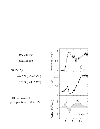
Figure 2: Single energy values of (a) inelasticities (triangles), (b) phase shift (circles) and best fit curves to phase shift (solid lines) in the $S_{11}$ partial wave of $\pi N$ elastic scattering and (c) distribution of time delay as a function of energy available in the $\pi N$ centre of mass system.

(note that in case there are several channels, the $S$-matrix is written as $\eta\exp(2i\delta)$) and the time delay. First of all we find sharp peaks at $1.5$ GeV and $1.65$ GeV corresponding to the well known resonances (Particle Data Group estimate of the pole value of the first $S_{11}$ resonance is $1.505$). Secondly, we get these peaks in spite of the small branching ratio of $S_{11}(1535)$ which is $Br(\pi N)=35-55\%$ and $Br(\eta N)=30-55\%$. It is also clear that the time delay becomes negative when the inelasticity parameter is largest. This can be understood as the loss of flux from the elastic channel due to the interpretation of $\Delta t$ as density of states [17]. In Figure 3 we have done a similar exercise for the $P_{11}$ case [18].

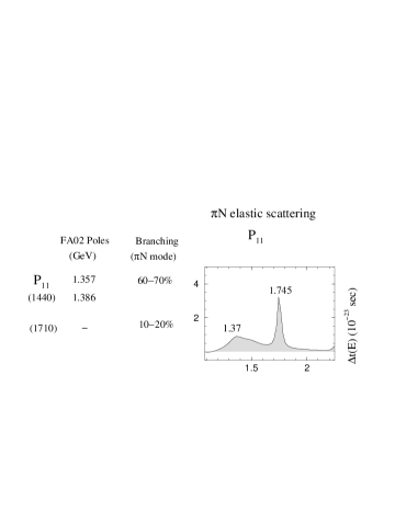
Figure 3: Time delay in the $P_{11}$ partial wave of $\pi N$ elastic scattering evaluated using the FA02 $T$-matrix solutions.

This is interesting from several points of view. Again we find two established resonances, but the focus is here on the three star $P_{11}(1710)$. We find this resonance by the time delay method at the right position even if the $\pi$N branching ratio is as small as $10-20\%$. We find it by using the FA02 [19] amplitudes even if the group which has performed the FA02 partial wave analysis cannot find the pole corresponding to $P_{11}(1710)$. Whether or not this resonance exists is important for the theoretical prediction of the mass of the Pentaquark $\Theta(1540)$ [20]. Indeed, this prediction relies on the existence of the $P_{11}(1710)$ [21]. Through the time delay method we find this resonance and also the Pentaquark [22] at the right positions.

In passing we note that even resonances like $P_{13}(1585)$, $G_{17}(2190)$ and $H_{19}(2220)$ with $\pi$N branching ratios of $10-20\%$ leave clear fingerprints in the time delay plots [18].

4 Resonances in $\pi\pi$ and $\pi K$ scattering

The previous sections showed that the time delay method is reliable in nuclear and baryon resonance physics. We now turn our attention to the mesonic case [23]. To show how reliable the method indeed is and how sensitive it is to small phase shift motion, we first apply the method to the case of the $\rho$-mesons. This is depicted in Figure 4.

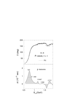
Figure 4: Time delay plot of the $\rho$ resonances evaluated from a fit to the p-wave phase shifts in $\pi\pi$ elastic scattering.

Evidently, we find the ‘not-to-be-missed’ $\rho(770)$, its first excitation $\rho(1450)$ and its second excitation $\rho(1700)$ which are all indisputable resonances. The peak at $1166$ MeV corresponds to a small phase motion and one could be tempted to disregard it as a fluctuation. However, several other cases, among others the three star resonance $D_{13}(1700)$ and the two star $F_{15}(2000)$, show that small phase shift ‘motion’ can signify a resonance. This seems to be the case also here. Particle Data Group lists also several mesons between $1100-2200$ MeV which by itself is not a remarkable fact. But at the recent Hadron 2001 conference in Protvino some authors have pointed out a growing evidence for a $\rho$-like resonance at $1200$ MeV which we think appears in our time delay plot[24]. Such a state has been also predicted in a coupled channel quark/meson model[25]. Our result in the $\rho$-meson sector is then an independent confirmation by the time delay method.

In the last few years the scalar sector attracted lots of attention. One of the reasons is the ‘re-discovery’ of the famous $\sigma$-meson and its ‘re-appearance’ in the Particle Data Book. The difficulty with this meson is reflected in the wide range of its possible mass, $400-1200$ MeV. The time delay analysis for this sector is summarized in Figure 5.

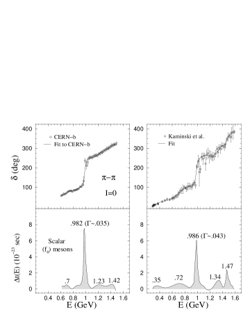
Figure 5: Time delay plot of the scalar meson resonances evaluated using two different sets of the s-wave phase shifts [26,27] in $\pi\pi$ elastic scattering.

Of course, $f_{0}(980)$ is a dominant contribution here. We identify the peak around $1.23(1.34)$ GeV with $f_{0}(1370)$ for which Particle Data Group quotes the range of possible pole mass between $1.2$ and $1.5$ GeV. Similarly the peak at $1.42(1.47)$ GeV is attributed to $f_{0}(1500)$ (the PDG value is $1.4-1.6$ GeV). The analysis of both phase shifts reveals a resonance at $700$ MeV. If, in addition, we take the information of the Kaminski phase shift we see also a peak at $350$ MeV. Can we take this as an evidence for two resonances? Let us first note that in the region of $400-1200$ where the $\sigma$-meson is found, one can identify two accumulation points. One at $350-600$ MeV and the other one at $700-850$ MeV. The low lying case is supported also by unitarized meson model[28], unitarized chiral perturbation theory [29] and by unitarized quark model [30], by coupled channel analysis[31] and by the so-called ABC effect [32] which is with us since 1961 and the recent decay $J/\Psi\to\sigma\omega\to\pi\pi\omega$ [33]. The $700$ MeV case finds its confirmation in Nambu-Jona-Lasinio models [34], Weinberg’s mended symmetry [35] and Bethe-Salpeter calculation [36]. Hence, these two accumulation points are not artificial constructs. They can be seen from the experimental results the theoretical expectation[37] so from the time delay method. Figure 6 serves as a cross check if the resonance found by the time delay method in the elastic channel finds its confirmation also in other channels. As can be seen this is indeed the case.

In the strange scalar sector the controversy regarding the lightest scalar (called $\kappa$ meson) is even bigger.

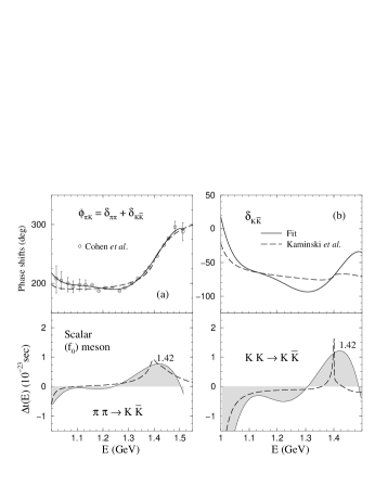
Figure 6: Energy dependence of the s-wave phase shifts and time delay in the (a) $\pi\pi\rightarrow K\bar{K}$ and (b) $K\bar{K}\rightarrow K\bar{K}$ reactions. The phase shifts $\delta_{K\bar{K}}$ (solid lines in (b)) have been determined by subtracting the fit to the CERN-b $\pi\pi$ phase shift data from $\phi_{\pi K}$ in the above figure (a). Dashed lines show the same quantities in the model calculation of [40].

Figure 7 is an analysis of this sector using two different phase shifts. This analysis also reveals the existence of two low lying resonances: one at $0.8$ GeV and the other around $1$ GeV which we identify with the putative $\kappa$-meson.

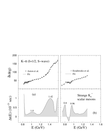
Figure 7: Time delay plots evaluated from the phase shifts in s-wave, isospin 1/2 $K\pi$ scattering, displaying the strange scalar mesons.

We have applied the time delay method to many ‘standard’ cases, the established baryon resonances, the $\rho$ mesons and the $K^{*}$- as well as $K_{2}^{*}$-mesons (discussed in [23]) and found a good agreement with data. Some less established resonances found by different methods get confirmed through the time delay method. By using the $KN$ phase shift we found the recently discovered Pentaquark with a mass very close to the observed and predicted value [22]. We found the spin-orbit partners of this Pentaquark very close to the theoretical expectations [38], [39]. Last but not least, our nuclear physics case discussed here in section two, shows also the virtues of the time delay method not only in finding nuclear levels, but also in studying the quantum evolution of unstable systems for large times.

References

- [1] See for example G. Kallen, Elementary Particle Physics, Addison-Wesley (1964).
- [2] S. Minami, Prog. Theor. Phys. 11, 213 (1954).
- [3] R. J. Cence, Pion-Nucleon Scattering, Princeton University Press (1969).
- [4] R. Kaminski, L. Lesniak and B. Loiseau, Phys. Lett B551, 241 (2003).
- [5] E. Beth and G. E. Uhlenbeck, Physica 4 (1937), 915 (1937); K. Huang, Statistical Mechanics, Wiley 1987.
- [6] N. S. Krylov, and V. A. Fock, JETP 17, 93 (1947).
- [7] H. Nakazato, M. Namiki and M. Pascazio, Int. J. Mod. Phys. B10, 247 (1996); A. Peres, Ann. Phys. (N.Y.) 129, 33 (1980); L. Fonda, G. C. Ghirardi and A. Rimini, Prog. Theor. Phys. 41, 587 (1978); K. Urbanowski, Phys. Rev. A50, 2847 (1994).
- [8] J. Bogdanowicz, M. Pindor, R. Raczka, Found. Phys. 25, 833 (1995); M. Nowakowski, Int. J. Mod. Phys. A 14, 589 (1999); J. Jankiewicz, hep-ph/0402268.
- [9] For an exhaustive list of phase shift data in the elastic - scattering via resonance see reference [10].
- [10] N. G. Kelkar, M. Nowakowski and K. P. Khemchandani, Phys. Rev. C70, 024601 (2004), nucl-th/0405043.
- [11] W. Broniowski, W. Florkowski and B. Hiller, Phys. Rev. 68 034911 (2003).
- [12] L. Eisenbud, dissertation, Princeton, June 1948 (unpublished); D. Bohm, Quantum Theory (1951) pp. 257-261; E. P. Wigner, Phys. Rev. 98, 145 (1955).
- [13] H. M. Nussenzveig, Causality and Dispersion Relations, Academic Press (1972).
- [14] M. Nowakowski and A. Pilaftsis, Z. Phys. C60, 121 (1993), hep-ph/9305321.
- [15] G. L. Morgan and R. L. Walter, Phys. Rev. D168, 114 (1968).
- [16] C. Garcia-Recio, J. Nieves, E. Ruiz Arriola and M. J. Vicente Vacas, Phys. Rev. D67, 076009 (2003).
- [17] N. G. Kelkar, J. Phys G: Nucl. Part. Phys. 29, L1 (2003), hep-ph/0205188.
- [18] N. G. Kelkar, M. Nowakowski, K. P. Khemchandani and S. R. Jain, Nucl. Phys. A 730, 121 (2004), hep-ph/0208197.
- [19] FA02 Partial Wave Analysis at http:// gwdac.phys.gwu.edu (We thank A. Arndt and I. I. Strakovsky for providing us the pole values of their analysis).
- [20] T. Nakano et al., Phys. Rev. Lett. 91, 012002 (2003).
- [21] D. Diakonov, V. Petrov and M. Polyakov, Z. Pys. A359, 305 (1997).
- [22] N. G. Kelkar, M. Nowakowski, and K. P. Khemchandani, J. Phys. G: Nucl. Part. Phys. 29, 1001 (2003), hep-ph/0307134.
- [23] N. G. Kelkar, M. Nowakowski and K. P. Khemchandani, Nucl. Phys. A 724, 357 (2003), hep-ph/0307184.
- [24] M. Achasov, hep-ex/0109035; B. Pick, Crystal Barrel Collaboration; A. Donnachie and Yu. S. Kalashnikova, hep-ph/0110191.
- [25] E. van Bevern, G. Rupp, T. A. Rijken and C. Dullemond, Phys. Rev. D27, 1527 (1983).
- [26] G. Grayer et al., Nucl. Phys. B75, 189 (1974).
- [27] R. Kaminski, L. Lesniak and K, Rybicki, Z. Phys. C74, 79 (1997).
- [28] E. van Beveren et al., Z. Phys. C30, 615 (1986).
- [29] A. Dobado and J. R. Pelaez, Phys. Rev. D56, 3057 (1997); J. A. Oller and E. Oset, Nucl. Phys. A620, 438 (1997).
- [30] N. A. Törnqvist and M. Roos, Phys. Rev. Lett. 77, 2332 (1996).
- [31] V. E. Markushin and M. P. Locher, hep-ph/9906249.
- [32] N. E. Booth, A. Abashian and K. M. Crowe, Phys. Rev. Lett. 7, 35 (1961); J. Yonnet et al., Phys. Rev. C63, 014001 (2001).
- [33] N. Wu, Recontre de Moriond, 2001, hep-ex/0104050; L. Roca, J. E. Palomar, E. Oset and H. C. Chiang, hep-ph/0405228.
- [34] Y. Nambu, G. Jona-Lasinio, Phys. Rev. 122, 345 (1961).
- [35] M. Svec, hep-ph/0209323; S. Weinberg, Phys. Rev. Lett. 65, 1177 (1990).
- [36] C. J. Burden at al, Phys. Rev. C55, 2649 (1997).
- [37] D. V. Bugg, Phys. Rep. 397, 257 (2004); E. van Beveren and G. Rupp, hep-ph/0201006.
- [38] N. G. Kelkar, M. Nowakowski and K. P. Khemchandani, Mod. Phys. Lett. A19, 2001 (2004), nucl-th/0405008.
- [39] N. G. Kelkar and M. Nowakowski, in this Proceedings, hep-ph/0412240.
- [40] R. Kaminski, L. Lesniak and B. Loiseau, Eur. Phys. J. C9, 141 (1999).