Abstract

The present lectures contain an introduction to possible new physics beyond the Standard Model. Having in mind first of all accelerator experiments of the nearest future we concentrate on supersymmetry, a new symmetry that relates bosons and fermions, as the first target of experimental search. Since supersymmetry is widely covered in the literature, we mostly consider novel developments and applications to hadron colliders. We describe then the so-called extra dimensional models in less detail and discuss their possible manifestations.

Preface

When discussing physics beyond the Standard Model one enters terra incognita and inevitably has to make some choice of the topic. When doing so I had in mind that most of the audience is working in one of the LHC collaborations and apparently is looking forward to discover new physics there. So their main goal will be to find the Higgs boson and then … who knows? Search for SUSY is the main stream and the general belief is that low energy supersymmetry described by the MSSM is round the corner. So one has to be prepared. The other widely discussed topic is extra dimensions. This is a much less motivated subject though is very intriguing. And if supersymmetry is already elaborated in detail and may be the subject of precise tests, extra dimensional models are more speculative and may bring many surprises or … nothing.

Supersymmetry has already more than 30 years of history and is very widely covered in the literature [1] and in the text books [2]-[5]. Moreover, I myself gave lectures on SUSY at the 2000 European School on High Energy Physics and they are published in the proceedings and are available in the web [6]. So I decided not to repeat the whole subject but keep the main line and to concentrate on the novel developments. In the year 2000 LEP was still running and obviously our main expectations to discover supersymmetry were connected with it. Unfortunately this did not happen. Today we are looking forward at hadron colliders and this is my main concern in these lectures. At the same time recent years celebrated unprecedented development in astroparticle experiments. This is the new area to look for new physics and in particular for the manifestation of SUSY. Therefore, I cover partly the motivations of SUSY in astrophysics and the influence of new astroparticle data on SUSY models.

When choosing the topic of extra dimensions I am aware of the fact that this deserves special lectures. At the same time, this subject is still an actively developing field and many changes in the ideas and preferences are possible. So I decided to make some overview without discussing theoretical problems (which are many) and to present possible experimental signatures since people are already looking for them. I do not pretend here for any complete coverage, my aim is to give the flavour of the field.

———————————————————–

^† Lectures given at the European School on High Energy Physics, May-June 2004,
Sant Feliu de Guixols, Spain

References 49

1 PART I   SUPERSYMMETRY

1.1 Introduction: What is supersymmetry

Supersymmetry is a boson-fermion symmetry that is aimed to unify all forces in Nature including gravity within a singe framework. Modern views on supersymmetry in particle physics are based on string paradigm, though the low energy manifestations of SUSY can be possibly found at modern colliders and in non-accelerator experiments.

Supersymmetry emerged from the attempts to generalize the Poincaré algebra to mix representations with different spin [7]. It happened to be a problematic task due to the no-go theorems preventing such generalizations [8]. The way out was found by introducing the so-called graded Lie algebras, i.e. adding the anti-commutators to the usual commutators of the Lorentz algebra. Such a generalization, described below, appeared to be the only possible one within relativistic field theory.

If $Q$ is a generator of SUSY algebra, then acting on a boson state it produces a fermion one and vice versa

$$\bar{Q}|boson>=|fermion>\ \ \ {\rm and}\ \ \ Q|fermion>=|boson>.$$

Since bosons commute with each other and fermions anticommute, one immediately finds that SUSY generators should also anticommute, they must be fermionic, i.e. they must change the spin by a half-odd amount and change the statistics. Indeed, the key element of SUSY algebra is

$$\{Q_{\alpha},\bar{Q}_{\dot{\alpha}}\}=2\sigma_{\alpha,\dot{\alpha}}^{\mu}P_{\mu},$$ (1.1)

where $Q$ and $\bar{Q}$ are SUSY generators and $P_{\mu}$ is the generator of translation, the four-momentum.

In what follows we describe SUSY algebra in more detail and construct its representations which are needed to build a SUSY generalization of the Standard Model of fundamental interactions. Such a generalization is based on a softly broken SUSY quantum filed theory and contains the SM as a low energy theory.

Supersymmetry promises to solve some problems of the SM and of Grand Unified Theories. In what follows we describe supersymmetry as a nearest option for the new physics on a TeV scale.

1.2 Motivation of SUSY in particle physics

There are several motivations of introduction of SUSY in particle physics. Most of them are related to ideas of unification of all the forces of Nature within the same framework. The incomplete set is:

$\bullet$ Unification with gravity

$\bullet$ Unification of gauge couplings

$\bullet$ Solution of the hierarchy problem

$\bullet$ Superstring consistency

$\bullet$ Dark Matter in the Universe

Probably the most challenging is the unification with gravity which is believed to happen within supergravity which in its turn is the low energy limit of a string theory. I have considered these arguments in some detail in my lectures [6] and will not repeat it here. Instead I will concentrate on the last motivation which became popular in recent time due to new data coming from astroparticle experiments.

1.2.1 Astrophysics and Cosmology

The shining matter is not the only one in the Universe. Considerable amount consists of the so-called dark matter. The direct evidence for the presence of the dark matter are the rotation curves of galaxies (see Fig.1) [9].

Figure 1: Rotation curves for the solar system and galaxy

What is shown here is the rotation speed of the planets of the solar system (left) and the stars in some typical spiral galaxy (right) as a function of a distance from the sun/center of galaxy. One can see that in the solar system all the planets perfectly fit the curve obtained from Newton mechanics: centrifugal force is equal to gravitational force

$$\frac{mv^{2}}{r}=G\frac{mM}{r^{2}},\ \ \Rightarrow\ \ v=\sqrt{\frac{GM}{r}}.$$

At the same time, if one looks at stars in the galaxy, one finds A completely different picture. To explain these curves, one has to assume the existence of galactic halo made of non shining matter which takes part in gravitational interaction. The flat rotation curves of spiral galaxies provide the most direct evidence for the existence of A large amount of the dark matter. Spiral galaxies consist of a central bulge and a very thin disc, and are surrounded by an approximately spherical halo of the dark matter.

According to the latest data [10], the matter content of the Universe is the following:

$$\Omega h^{2}=1\ \ \Leftrightarrow\ \ \rho=\rho_{crit}$$

$$\Omega_{vacuum}\approx 73\%,\ \ \Omega_{DarkMatter}\approx 23\%,\ \ \Omega_{Baryon}\approx 4\%$$

Therefore, the amount of the Dark matter is almost 6 times larger than the usual matter in the Universe.

There are two possible types of the dark matter: the hot one, consisting of light relativistic particles and the cold one, consisting of massive weakly interacting particles (WIMPs). The hot dark matter might consist of neutrinos; however, this has problems with galaxy formation. As for the cold dark matter, it has no candidates within the SM. At the same time, SUSY provides an excellent candidate for the cold dark matter, namely neutralino, the lightest superparticle.

1.3 Basics of supersymmetry

Sending off the interested reader to [6] for details we present here the main ideas and building blocks for constructing a supersymmetric quantum field theory.

1.3.1 Algebra of SUSY

Combined with the usual Poincaré and internal symmetry algebra the Super-Poincaré Lie algebra contains additional SUSY generators $Q_{\alpha}^{i}$ and $\bar{Q}_{\dot{\alpha}}^{i}$ [2]

$$\begin{array}[]{l}{[}P_{\mu},P_{\nu}{]}=0,\\ {[}P_{\mu},M_{\rho\sigma}{]}=i(g_{\mu\rho}P_{\sigma}-g_{\mu\sigma}P_{\rho}),\\ {[}M_{\mu\nu},M_{\rho\sigma}{]}=i(g_{\nu\rho}M_{\mu\sigma}-g_{\nu\sigma}M_{\mu\rho}-g_{\mu\rho}M_{\nu\sigma}+g_{\mu\sigma}M_{\nu\rho}),\\ {[}B_{r},B_{s}{]}=iC_{rs}^{t}B_{t},\\ {[}B_{r},P_{\mu}{]}={[}B_{r},M_{\mu\sigma}{]}=0,\\ {[}Q_{\alpha}^{i},P_{\mu}{]}={[}\bar{Q}_{\dot{\alpha}}^{i},P_{\mu}{]}=0,\\ {[}Q_{\alpha}^{i},M_{\mu\nu}{]}=\frac{1}{2}(\sigma_{\mu\nu})_{\alpha}^{\beta}Q_{\beta}^{i},\ \ \ \ {[}\bar{Q}_{\dot{\alpha}}^{i},M_{\mu\nu}{]}=-\frac{1}{2}\bar{Q}_{\dot{\beta}}^{i}(\bar{\sigma}_{\mu\nu})_{\dot{\alpha}}^{\dot{\beta}},\\ {[}Q_{\alpha}^{i},B_{r}{]}=(b_{r})_{j}^{i}Q_{\alpha}^{j},\ \ \ {[}\bar{Q}_{\dot{\alpha}}^{i},B_{r}{]}=-\bar{Q}_{\dot{\alpha}}^{j}(b_{r})_{j}^{i},\\ \{Q_{\alpha}^{i},\bar{Q}_{\dot{\beta}}^{j}\}=2\delta^{ij}(\sigma^{\mu})_{\alpha\dot{\beta}}P_{\mu},\\ \{Q_{\alpha}^{i},Q_{\beta}^{j}\}=2\epsilon_{\alpha\beta}Z^{ij},\ \ \ Z_{ij}=a_{ij}^{r}b_{r},\ \ \ \ Z^{ij}=Z_{ij}^{+},\\ \{\bar{Q}_{\dot{\alpha}}^{i},\bar{Q}_{\dot{\beta}}^{j}\}=-2\epsilon_{\dot{\alpha}\dot{\beta}}Z^{ij},\ \ \ {[}Z_{ij},anything{]}=0,\\ \alpha,\dot{\alpha}=1,2\ \ \ \ i,j=1,2,\ldots,N.\end{array}$$ (1.2)

Here $P_{\mu}$ and $M_{\mu\nu}$ are four-momentum and angular momentum operators, respectively, $B_{r}$ are the internal symmetry generators, $Q^{i}$ and $\bar{Q}^{i}$ are the spinorial SUSY generators and $Z_{ij}$ are the so-called central charges; $\alpha,\dot{\alpha},\beta,\dot{\beta}$ are the spinorial indices. In the simplest case one has one spinor generator $Q_{\alpha}$ (and the conjugated one $\bar{Q}_{\dot{\alpha}}$) that corresponds to an ordinary or N=1 supersymmetry. When $N>1$ one has an extended supersymmetry. In what follows we consider the simplest N=1 case used for phenomenology.

To construct the representations of SUSY algebra (particle states in SUSY model) we start with the some state labeled by energy and helicity, i.e. projection of a spin on the direction of momenta

$$|E,\lambda>$$

and act on it with the SUSY generator $\bar{Q}$. Then one obtains the other state with the same energy (because SUSY generator commutes with $P_{\mu}$) but different helicity

$$\bar{Q}|E,\lambda>=|E,\lambda+1/2>.$$ (1.3)

Due to the nilpotent character of SUSY generators (1.2), the repeated action of the generator $\bar{Q}$ gives zero. This is common for N=1 SUSY. One has two states, one bosonic and one fermionic. This is a generic property of any supersymmetric theory that the number of bosons equals that of fermions. However, in CPT invariant theories the number of states is doubled, since CPT transformation changes the sign of helicity. Hence, in CPT invariant theories, one has to add the states with opposite helicity to the above mentioned ones.

Consider some examples. Let us take $\lambda=0$. Then one has the following complete multiplet of SUSY:

$$\begin{array}[]{lccccccc}&\mbox{helicity}&0&1/2&&\mbox{helicity}&0&-1/2\\ N=1\ \ \ \lambda=0&&&&\stackrel{{\scriptstyle CPT}}{{\Longrightarrow}}&&&\\ &\#\ \mbox{of states}&1&1&&\#\ \mbox{of states}&1&1\end{array}$$

which contains one complex scalar and one spinor with two helicity states.

The other multiplet can be obtained if one starts with $\lambda=1/2$. Then one has:

$$\begin{array}[]{lccccccc}&\mbox{helicity}&1/2&1&&\mbox{helicity}&-1&1/2\\ N=1\ \ \ \lambda=1/2&&&&\stackrel{{\scriptstyle CPT}}{{\Longrightarrow}}&&&\\ &\#\ \mbox{of states}&1&1&&\#\ \mbox{of states}&1&1\end{array}$$

This multiplet contains one spinor field and one massless vector.

Thus, one has two types of supermultiplets: the so-called chiral multiplet with $\lambda=0$, which contains two physical states $(\phi,\psi)$ with spin 0 and 1/2, respectively, and the vector multiplet with $\lambda=1/2$, which also contains two physical states $(\lambda,A_{\mu})$ with spin 1/2 and 1, respectively. These multiplets are used to describe quarks, leptons and vector bosons in SUSY generalization of the SM.

1.3.2 Superspace and superfields

An elegant formulation of supersymmetry transformations and invariants can be achieved in the framework of superspace [3]. Superspace differs from the ordinary Euclidean (Minkowski) space by adding of two new coordinates, $\theta_{\alpha}$ and $\bar{\theta}_{\dot{\alpha}}$, which are Grassmannian, i.e. anticommuting, variables

$$\{\theta_{\alpha},\theta_{\beta}\}=0,\ \ \{\bar{\theta}_{\dot{\alpha}},\bar{\theta}_{\dot{\beta}}\}=0,\ \ \theta_{\alpha}^{2}=0,\ \ \bar{\theta}_{\dot{\alpha}}^{2}=0,\ \ \alpha,\beta,\dot{\alpha},\dot{\beta}=1,2.$$

Thus, we go from space to superspace

$$\begin{array}[]{cc}Space&\ \Rightarrow\ \ Superspace\\ x_{\mu}&\ \ \ \ \ \ \ x_{\mu},\theta_{\alpha},\bar{\theta}_{\dot{\alpha}}\end{array}$$

Supersymmetry transformation in superspace looks like an ordinary translation but in Grassmannian coordinates

$$\begin{array}[]{ccl}x_{\mu}&\rightarrow&x_{\mu}+i\theta\sigma_{\mu}\bar{\varepsilon}-i\varepsilon\sigma_{\mu}\bar{\theta},\\ \theta&\rightarrow&\theta+\varepsilon,\ \ \bar{\theta}\rightarrow\bar{\theta}+\bar{\varepsilon},\end{array}$$ (1.4)

where $\varepsilon$ and $\bar{\varepsilon}$ are Grassmannian transformation parameters. From eq.(1.4) one can easily obtain the representation for the supercharges (1.2), the generators of supersymmetry, acting on the superspace

$$Q_{\alpha}=\frac{\partial}{\partial\theta_{\alpha}}-i\sigma^{\mu}_{\alpha\dot{\alpha}}\bar{\theta}^{\dot{\alpha}}\partial_{\mu},\ \ \ \bar{Q}_{\dot{\alpha}}=-\frac{\partial}{\partial\bar{\theta}_{\dot{\alpha}}}+i\theta_{\alpha}\sigma^{\mu}_{\alpha\dot{\alpha}}\partial_{\mu}.$$ (1.5)

To define the fields on a superspace, consider representations of the Super-Poincaré group (1.2) [2]. The simplest N=1 SUSY multiplets that we discussed earlier are: the chiral one $\Phi(y,\theta)$ ($y=x+i\theta\sigma\bar{\theta}$) and the vector one $V(x,\theta,\bar{\theta})$. Being expanded in Taylor series over Grassmannian variables $\theta$ and $\bar{\theta}$ they give:

$$\Phi(y,\theta) = A(y)+\sqrt{2}\theta\psi(y)+\theta\theta F(y)$$

$$= A(x)+i\theta\sigma^{\mu}\bar{\theta}\partial_{\mu}A(x)+\frac{1}{4}\theta\theta\bar{\theta}\bar{\theta}\Box A(x)$$

$$+ \sqrt{2}\theta\psi(x)-\frac{i}{\sqrt{2}}\theta\theta\partial_{\mu}\psi(x)\sigma^{\mu}\bar{\theta}+\theta\theta F(x).$$

The coefficients are ordinary functions of $x$ being the usual fields. They are called the components of a superfield. In eq.(1.3.2) one has 2 bosonic (complex scalar field $A$) and 2 fermionic (Weyl spinor field $\psi$) degrees of freedom. The component fields $A$ and $\psi$ are called the superpartners. The field $F$ is an auxiliary field, it has the ”wrong” dimension and has no physical meaning. It is needed to close the algebra (1.2). One can get rid of the auxiliary fields with the help of equations of motion.

Thus, a superfield contains an equal number of bosonic and fermionic degrees of freedom. Under SUSY transformation they convert into one another

$$\delta_{\varepsilon}A = \sqrt{2}\varepsilon\psi,$$

$$\delta_{\varepsilon}\psi = i\sqrt{2}\sigma^{\mu}\bar{\varepsilon}\partial_{\mu}A+\sqrt{2}\varepsilon F,$$ (1.7)

$$\delta_{\varepsilon}F = i\sqrt{2}\bar{\varepsilon}\sigma^{\mu}\partial_{\mu}\psi.$$

Notice that the variation of the $F$-component is a total derivative, i.e. it vanishes when integrated over the space-time.

The vector superfield is real $V=V^{+}$. It has the following Grassmannian expansion:

$$V(x,\theta,\bar{\theta}) = C(x)+i\theta\chi(x)-i\bar{\theta}\bar{\chi}(x)+\frac{i}{2}\theta\theta[M(x)+iN(x)]$$ (1.8)

$$-\ \frac{i}{2}\bar{\theta}\bar{\theta}[M(x)-iN(x)]-\theta\sigma^{\mu}\bar{\theta}v_{\mu}(x)+i\theta\theta\bar{\theta}[\lambda(x)+\frac{i}{2}\bar{\sigma}^{\mu}\partial_{\mu}\chi(x)]$$

$$- i\bar{\theta}\bar{\theta}\theta[\lambda+\frac{i}{2}\sigma^{\mu}\partial_{\mu}\bar{\chi}(x)]+\frac{1}{2}\theta\theta\bar{\theta}\bar{\theta}[D(x)+\frac{1}{2}\Box C(x)].$$

The physical degrees of freedom corresponding to a real vector superfield $V$ are the vector gauge field $v_{\mu}$ and the Majorana spinor field $\lambda$. All other components are unphysical and can be eliminated. Indeed, one can choose a gauge (the Wess-Zumino gauge) where $C=\chi=M=N=0$, leaving one with only physical degrees of freedom except for the auxiliary field $D$. In this gauge

$$V = -\theta\sigma^{\mu}\bar{\theta}v_{\mu}(x)+i\theta\theta\bar{\theta}\bar{\lambda}(x)-i\bar{\theta}\bar{\theta}\theta\lambda(x)+\frac{1}{2}\theta\theta\bar{\theta}\bar{\theta}D(x),$$

$$V^{2} = -\frac{1}{2}\theta\theta\bar{\theta}\bar{\theta}v_{\mu}(x)v^{\mu}(x),$$

$$V^{3} = 0,\ \ \ etc.$$ (1.9)

One can define also a field strength tensor (as analog of $F_{\mu\nu}$ in gauge theories)

$$W_{\alpha}=-\frac{1}{4}\bar{D}^{2}e^{V}D_{\alpha}e^{-V},\ \ \ \ \bar{W}_{\dot{\alpha}}=-\frac{1}{4}D^{2}e^{V}\bar{D}_{\alpha}e^{-V},$$ (1.10)

Here $Ds$ are the supercovariant derivatives. In the Wess-Zumino gauge the strength tensor is a polynomial over component fields:

$$W_{\alpha}=T^{a}\left(-i\lambda^{a}_{\alpha}+\theta_{\alpha}D^{a}-\frac{i}{2}(\sigma^{\mu}\bar{\sigma}^{\nu}\theta)_{\alpha}F^{a}_{\mu\nu}+\theta^{2}(\sigma^{\mu}D_{\mu}\bar{\lambda}^{a})_{\alpha}\right),$$ (1.11)

where

$$F^{a}_{\mu\nu}=\partial_{\mu}v^{a}_{\nu}-\partial_{\nu}v^{a}_{\mu}+f^{abc}v^{b}_{\mu}v^{c}_{\nu},\ \ \ D_{\mu}\bar{\lambda}^{a}=\partial\bar{\lambda}^{a}+f^{abc}v^{b}_{\mu}\bar{\lambda}^{c}.$$

In Abelian case eqs.(1.10) are simplified and take form

$$W_{\alpha}=-\frac{1}{4}\bar{D}^{2}D_{\alpha}V,\ \ \ \bar{W}_{\dot{\alpha}}=-\frac{1}{4}D^{2}\bar{D}_{\alpha}V.$$

1.3.3 Construction of SUSY Lagrangians

Let us start with the Lagrangian which has no local gauge invariance. In the superfield notation SUSY invariant Lagrangians are the polynomials of superfields. The same way as an ordinary action is an integral over space-time of Lagrangian density, in supersymmetric case the action is an integral over the superspace. The space-time Lagrangian density is [2, 3]

$${\cal L}=\int d^{2}\theta d^{2}\bar{\theta}~{}\Phi_{i}^{+}\Phi_{i}+\int d^{2}\theta~{}[\lambda_{i}\Phi_{i}+\frac{1}{2}m_{ij}\Phi_{i}\Phi_{j}+\frac{1}{3}y_{ijk}\Phi_{i}\Phi_{j}\Phi_{k}]+h.c.$$ (1.12)

where the first part is a kinetic term and the second one is a superpotential ${\cal W}$. We use here integration over the superspace according to the rules of Grassmannian integration [11]

$$\int\ d\theta_{\alpha}=0,\ \ \ \ \int\theta_{\alpha}\ d\theta_{\beta}=\delta_{\alpha\beta}.$$

Performing explicit integration over the Grassmannian parameters, we get from eq.(1.12)

$${\cal L} = i\partial_{\mu}\bar{\psi}_{i}\bar{\sigma}^{\mu}\psi_{i}+A_{i}^{\ast}\Box A_{i}+F_{i}^{\ast}F_{i}$$

$$+ [\lambda_{i}F_{i}+m_{ij}(A_{i}F_{j}-\frac{1}{2}\psi_{i}\psi_{j})+y_{ijk}(A_{i}A_{j}F_{k}-\psi_{i}\psi_{j}A_{k})+h.c.].$$

The last two terms are the interaction ones. To obtain a familiar form of the Lagrangian, we have to solve the constraints

$$\frac{\partial{\cal L}}{\partial F_{k}^{*}} = F_{k}+\lambda_{k}^{*}+m_{ik}^{*}A_{i}^{*}+y_{ijk}^{*}A_{i}^{*}A_{j}^{*}=0,$$ (1.14)

$$\frac{\partial{\cal L}}{\partial F_{k}} = F_{k}^{*}+\lambda_{k}+m_{ik}A_{i}+y_{ijk}A_{i}A_{j}=0.$$ (1.15)

Expressing the auxiliary fields $F$ and $F^{*}$ from these equations, one finally gets

$${\cal L} = i\partial_{\mu}\bar{\psi}_{i}\bar{\sigma}^{\mu}\psi_{i}+A_{i}^{*}\Box A_{i}-\frac{1}{2}m_{ij}\psi_{i}\psi_{j}-\frac{1}{2}m_{ij}^{*}\bar{\psi}_{i}\bar{\psi}_{j}$$ (1.16)

$$-y_{ijk}\psi_{i}\psi_{j}A_{k}-y_{ijk}^{*}\bar{\psi}_{i}\bar{\psi}_{j}A_{k}^{*}-V(A_{i},A_{j}),$$

where the scalar potential $V=F_{k}^{*}F_{k}$. We will return to the discussion of the form of the scalar potential in SUSY theories later.

Consider now the gauge invariant SUSY Lagrangians. They should contain gauge invariant interaction of the matter fields with the gauge ones and the kinetic term and the self-interaction of the gauge fields.

Let us start with the gauge field kinetic terms. In the Wess-Zumino gauge one has

$$W^{\alpha}W_{\alpha}|_{\theta\theta}=-2i\lambda\sigma^{\mu}D_{\mu}\bar{\lambda}-\frac{1}{2}F_{\mu\nu}F^{\mu\nu}+\frac{1}{2}D^{2}+i\frac{1}{4}F^{\mu\nu}F^{\rho\sigma}\epsilon_{\mu\nu\rho\sigma},$$ (1.17)

where $D_{\mu}=\partial_{\mu}+ig[v_{\mu},]$ is the usual covariant derivative and the last, the so-called topological $\theta$ term, is the total derivative. The gauge invariant Lagrangian now has a familiar form

$${\cal L} = \frac{1}{4}\int d^{2}\theta~{}W^{\alpha}W_{\alpha}+\frac{1}{4}\int d^{2}\bar{\theta}~{}\bar{W}^{\dot{\alpha}}\bar{W}_{\dot{\alpha}}$$ (1.18)

$$= \frac{1}{2}D^{2}-\frac{1}{4}F_{\mu\nu}F^{\mu\nu}-i\lambda\sigma^{\mu}D_{\mu}\bar{\lambda}.$$

To obtain a gauge-invariant interaction with matter chiral superfields, one has to modify the kinetic term by inserting the bridge operator

$$\Phi_{i}^{+}\Phi_{i}\Rightarrow\Phi_{i}^{+}e^{gV}\Phi_{i}.$$ (1.19)

A complete SUSY and gauge invariant Lagrangian then looks like

$${\cal L}_{SUSY\ YM} = \frac{1}{4}\int d^{2}\theta~{}Tr(W^{\alpha}W_{\alpha})+\frac{1}{4}\int d^{2}\bar{\theta}~{}Tr(\bar{W}^{\alpha}\bar{W}_{\alpha})$$

$$+ \int d^{2}\theta d^{2}\bar{\theta}~{}\bar{\Phi}_{ia}(e^{gV})_{b}^{a}\Phi_{i}^{b}+\int d^{2}\theta~{}{\cal W}(\Phi_{i})+\int d^{2}\bar{\theta}~{}\bar{{\cal W}}(\bar{\Phi}_{i}),$$

where ${\cal W}$ is a superpotential, which should be invariant under the group of symmetry of a particular model. In terms of component fields the above Lagrangian takes the form

$${\cal L}_{SUSY\ YM} = -\frac{1}{4}F^{a}_{\mu\nu}F^{a\mu\nu}-i\lambda^{a}\sigma^{\mu}D_{\mu}\bar{\lambda}^{a}+\frac{1}{2}D^{a}D^{a}$$

$$+\ (\partial_{\mu}A_{i}-igv^{a}_{\mu}T^{a}A_{i})^{\dagger}(\partial_{\mu}A_{i}-igv^{a}_{\mu}T^{a}A_{i})-i\bar{\psi}_{i}\bar{\sigma}^{\mu}(\partial_{\mu}\psi_{i}-igv^{a}_{\mu}T^{a}\psi_{i})$$

$$-\ D^{a}A^{\dagger}_{i}T^{a}A_{i}-i\sqrt{2}A^{\dagger}_{i}T^{a}\lambda^{a}\psi_{i}+i\sqrt{2}\bar{\psi}_{i}T^{a}A_{i}\bar{\lambda}^{a}+F^{\dagger}_{i}F_{i}$$

$$+\ \frac{\partial{\cal W}}{\partial A_{i}}F_{i}+\frac{\partial\bar{{\cal W}}}{\partial A_{i}^{\dagger}}F^{\dagger}_{i}-\frac{1}{2}\frac{\partial^{2}{\cal W}}{\partial A_{i}\partial A_{j}}\psi_{i}\psi_{j}-\frac{1}{2}\frac{\partial^{2}\bar{{\cal W}}}{\partial A_{i}^{\dagger}\partial A_{j}^{\dagger}}\bar{\psi}_{i}\bar{\psi}_{j}.$$

Integrating out the auxiliary fields $D^{a}$ and $F_{i}$, one reproduces the usual Lagrangian.

1.3.4 The scalar potential

Contrary to the SM, where the scalar potential is arbitrary and is defined only by the requirement of the gauge invariance, in supersymmetric theories it is completely defined by the superpotential. It consists of the contributions from the $D$-terms and $F$-terms. The kinetic energy of the gauge fields (recall eq.(1.18) yields the $1/2D^{a}D^{a}$ term, and the matter-gauge interaction (recall eq.(1.3.3) yields the $gD^{a}T^{a}_{ij}A^{*}_{i}A_{j}$ one. Together they give

$${\cal L}_{D}=\frac{1}{2}D^{a}D^{a}+gD^{a}T^{a}_{ij}A^{*}_{i}A_{j}.$$ (1.22)

The equation of motion reads

$$D^{a}=-gT^{a}_{ij}A^{*}_{i}A_{j}.$$ (1.23)

Substituting it back into eq.(1.22) yields the $D$-term part of the potential

$${\cal L}_{D}=-\frac{1}{2}D^{a}D^{a}\ \ \ \ \Longrightarrow V_{D}=\frac{1}{2}D^{a}D^{a},$$ (1.24)

where $D$ is given by eq.(1.23).

The $F$-term contribution can be derived from the matter field self-interaction eq.(1.3.3). For a general type superpotential $W$ one has

$${\cal L}_{F}=F^{*}_{i}F_{i}+(\frac{\partial W}{\partial A_{i}}F_{i}+h.c.).$$ (1.25)

Using the equations of motion for the auxiliary field $F_{i}$

$$F^{*}_{i}=-\frac{\partial W}{\partial A_{i}}$$ (1.26)

yields

$${\cal L}_{F}=-F^{*}_{i}F_{i}\ \ \ \ \Longrightarrow V_{F}=F^{*}_{i}F_{i},$$ (1.27)

where $F$ is given by eq.(1.26). The full potential is the sum of the two contributions

$$V=V_{D}+V_{F}.$$ (1.28)

Thus, the form of the Lagrangian is practically fixed by symmetry requirements. The only freedom is the field content, the value of the gauge coupling $g$, Yukawa couplings $y_{ijk}$ and the masses. Because of the renormalizability constraint $V\leq A^{4}$ the superpotential should be limited by ${\cal W}\leq\Phi^{3}$ as in eq.(1.12). All members of a supermultiplet have the same masses, i.e. bosons and fermions are degenerate in masses. This property of SUSY theories contradicts the phenomenology and requires supersymmetry breaking.

1.3.5 Spontaneous breaking of SUSY

Since supersymmetric algebra leads to mass degeneracy in a supermultiplet, it should be broken to explain the absence of superpartners at modern energies. There are several ways of supersymmetry breaking. It can be broken either explicitly or spontaneously. Performing SUSY breaking one has to be careful not to spoil the cancellation of quadratic divergencies which allows one to solve the hierarchy problem. This is achieved by spontaneous breaking of SUSY.

Apart from non-supersymmetric theories, in SUSY models the energy is always nonnegative definite. Indeed, according to quantum mechanics

$$E=<0|\ H\ |0>$$

and due to SUSY algebra eq.(1.2) $\{Q_{\alpha},\bar{Q}_{\dot{\beta}}\}=2(\sigma^{\mu})_{\alpha\dot{\beta}}P_{\mu},$ taking into account that $tr(\sigma^{\mu}P_{\mu})=2P_{0},$ one gets

$$E=\frac{1}{4}\sum_{\alpha=1,2}<0|\{Q_{\alpha},\bar{Q}_{\alpha}\}|0>=\frac{1}{4}\sum_{\alpha}|Q_{\alpha}|0>|^{2}\geq 0.$$

Hence

$$E=<0|\ H\ |0>\neq 0\ \ \ \ if\ and\ only\ if\ \ \ Q_{\alpha}|0>\neq 0.$$

Therefore, supersymmetry is spontaneously broken, i.e. vacuum is not invariant $(Q_{\alpha}|0>\neq 0)$, if and only if the minimum of the potential is positive $(i.e.\ E>0)$ .

Spontaneous breaking of supersymmetry is achieved in the same way as the electroweak symmetry breaking. One introduces the field whose vacuum expectation value is nonzero and breaks the symmetry. However, due to a special character of SUSY, this should be a superfield whose auxiliary $F$ and $D$ components acquire nonzero v.e.v.’s. Thus, among possible spontaneous SUSY breaking mechanisms one distinguishes the $F$ and $D$ ones.

i) Fayet-Iliopoulos ($D$-term) mechanism [12].
In this case the, the linear $D$-term is added to the Lagrangian

$$\Delta{\cal L}=\xi V|_{\theta\theta\bar{\theta}\bar{\theta}}=\xi\int d^{4}\theta\ V.$$ (1.29)

It is gauge and SUSY invariant by itself; however, it may lead to spontaneous breaking of both of them depending on the value of $\xi$. We show in Fig.2a the sample spectrum for two chiral matter multiplets.

Figure 2: Spectrum of spontaneously broken SUSY theories

The drawback of this mechanism is the necessity of $U(1)$ gauge invariance. It can be used in SUSY generalizations of the SM but not in GUTs.

The mass spectrum also causes some troubles since the following sum rule is valid

$$\sum_{bosonic\ states}m^{2}_{i}=\sum_{fermionic\ states}m^{2}_{i},$$ (1.30)

which is bad for phenomenology.

ii) O’Raifeartaigh ($F$-term) mechanism [13].
In this case, several chiral fields are needed and the superpotential should be chosen in a way that trivial zero v.e.v.s for the auxiliary $F$-fields be absent. For instance, choosing the superpotential to be

$${\cal W}(\Phi)=\lambda\Phi_{3}+m\Phi_{1}\Phi_{2}+g\Phi_{3}\Phi_{1}^{2},$$

one gets the equations for the auxiliary fields

$$F^{*}_{1} = mA_{2}+2gA_{1}A_{3},$$

$$F^{*}_{2} = mA_{1},$$

$$F^{*}_{3} = \lambda+gA^{2}_{1},$$

which have no solutions with $<F_{i}>=0$ and SUSY is spontaneously broken. The sample spectrum is shown in Fig.2b.

The drawbacks of this mechanism is a lot of arbitrariness in the choice of potential. The sum rule (1.30) is also valid here.

Unfortunately, none of these mechanisms explicitly works in SUSY generalizations of the SM. None of the fields of the SM can develop nonzero v.e.v.s for their $F$ or $D$ components without breaking $SU(3)$ or $U(1)$ gauge invariance since they are not singlets with respect to these groups. This requires the presence of extra sources of spontaneous SUSY breaking, which we consider below. They are based, however, on the same $F$ and $D$ mechanisms.

1.4 SUSY generalization of the Standard Model. The MSSM

As has been already mentioned, in SUSY theories the number of bosonic degrees of freedom equals that of fermionic. At the same time, in the SM one has 28 bosonic and 90 (96 with right handed neutrino) fermionic degrees of freedom. So the SM is to a great extent non-supersymmetric. Trying to add some new particles to supersymmetrize the SM, one should take into account the following observations:

$\bullet$ There are no fermions with quantum numbers of the gauge bosons;

$\bullet$ Higgs fields have nonzero v.e.v.s; hence they cannot be superpartners of quarks and leptons since this would induce spontaneous violation of baryon and lepton numbers;

$\bullet$ One needs at least two complex chiral Higgs multiplets to give masses to Up and Down quarks.

The latter is due to the form of a superpotential and chirality of matter superfields. Indeed, the superpotential should be invariant under the $SU(3)\times SU(2)\times U(1)$ gauge group. If one looks at the Yukawa interaction in the Standard Model, one finds that it is indeed $U(1)$ invariant since the sum of hypercharges in each vertex equals zero. In the last term this is achieved by taking the conjugated Higgs doublet $\tilde{H}=i\tau_{2}H^{\dagger}$ instead of $H$. However, in SUSY $H$ is a chiral superfield and hence a superpotential, which is constructed out of chiral fields, can contain only $H$ but not $\tilde{H}$ which is an antichiral superfield.

Another reason for the second Higgs doublet is related to chiral anomalies. It is known that chiral anomalies spoil the gauge invariance and, hence, the renormalizability of the theory. They are canceled in the SM between quarks and leptons in each generation. However, if one introduces a chiral Higgs superfield, it contains higgsinos, which are chiral fermions, and contain anomalies. To cancel them one has to add the second Higgs doublet with the opposite hypercharge. Therefore, the Higgs sector in SUSY models is inevitably enlarged, it contains an even number of doublets.

Conclusion: In SUSY models supersymmetry associates known bosons with new fermions and known fermions with new bosons.

1.4.1 The field content

Consider the particle content of the Minimal Supersymmetric Standard Model [14, 6]. According to the previous discussion, in the minimal version we double the number of particles (introducing a superpartner to each particle) and add another Higgs doublet (with its superpartner). Thus, the characteristic feature of any supersymmetric generalization of the SM is the presence of superpartners (see Fig.3). If supersymmetry is exact, superpartners of ordinary particles should have the same masses and have to be observed. The absence of them at modern energies is believed to be explained by the fact that their masses are very heavy, that means that supersymmetry should be broken.

Figure 3: The shadow world of SUSY particles [15]

The particle content of the MSSM then appears as (tilde denotes a superpartner of an ordinary particle).

Particle Content of the MSSM Superfield        Bosons        Fermions $SU_{c}(3)$ $SU_{L}(2)$ $U_{Y}(1)$ Gauge ${\bf G^{a}}$ gluon                 $g^{a}$ gluino$\ \ \ \ \ \ \ \ \ \ \ \ \tilde{g}^{a}$ 8 1 0 ${\bf V^{k}}$ Weak    $W^{k}$  $(W^{\pm},Z)$ wino, zino  $\tilde{w}^{k}$  $(\tilde{w}^{\pm},\tilde{z})$ 1 3 0 ${\bf V^{\prime}}$ Hypercharge    $B\ (\gamma)$ bino            $\tilde{b}(\tilde{\gamma})$ 1 1 0 Matter $\begin{array}[]{c}{\bf L_{i}}\\ {\bf E_{i}}\end{array}$ sleptons  $\left\{\begin{array}[]{l}\tilde{L}_{i}=(\tilde{\nu},\tilde{e})_{L}\\ \tilde{E}_{i}=\tilde{e}_{R}\end{array}\right.$ leptons  $\left\{\begin{array}[]{l}L_{i}=(\nu,e)_{L}\\ E_{i}=e_{R}\end{array}\right.$ $\begin{array}[]{l}1\\ 1\end{array}$ $\begin{array}[]{l}2\\ 1\end{array}$ $\begin{array}[]{r}-1\\ 2\end{array}$ $\begin{array}[]{c}{\bf Q_{i}}\\ {\bf U_{i}}\\ {\bf D_{i}}\end{array}$ squarks  $\left\{\begin{array}[]{l}\tilde{Q}_{i}=(\tilde{u},\tilde{d})_{L}\\ \tilde{U}_{i}=\tilde{u}_{R}\\ \tilde{D}_{i}=\tilde{d}_{R}\end{array}\right.$ quarks  $\left\{\begin{array}[]{l}Q_{i}=(u,d)_{L}\\ U_{i}=u_{R}^{c}\\ D_{i}=d_{R}^{c}\end{array}\right.$ $\begin{array}[]{l}3\\ 3^{*}\\ 3^{*}\end{array}$ $\begin{array}[]{l}2\\ 1\\ 1\end{array}$ $\begin{array}[]{r}1/3\\ -4/3\\ 2/3\end{array}$ Higgs $\begin{array}[]{c}{\bf H_{1}}\\ {\bf H_{2}}\end{array}$ Higgses  $\left\{\begin{array}[]{l}H_{1}\\ H_{2}\end{array}\right.$ higgsinos  $\left\{\begin{array}[]{l}\tilde{H}_{1}\\ \tilde{H}_{2}\end{array}\right.$ $\begin{array}[]{l}1\\ 1\end{array}$ $\begin{array}[]{l}2\\ 2\end{array}$ $\begin{array}[]{r}-1\\ 1\end{array}$

The presence of an extra Higgs doublet in SUSY model is a novel feature of the theory. In the MSSM one has two doublets with the quantum numbers (1,2,-1) and (1,2,1), respectively:

$$H_{1}=\left(\begin{array}[]{c}H^{0}_{1}\\ H_{1}^{-}\end{array}\right)=\left(\begin{array}[]{c}v_{1}+\frac{S_{1}+iP_{1}}{\sqrt{2}}\\ H^{-}_{1}\end{array}\right),\ H_{2}=\left(\begin{array}[]{c}H^{+}_{2}\\ H_{2}^{0}\end{array}\right)=\left(\begin{array}[]{c}H^{+}_{2}\\ v_{2}+\frac{S_{2}+iP_{2}}{\sqrt{2}}\end{array}\right),$$

where $v_{i}$ are the vacuum expectation values of the neutral components.

Hence, one has 8=4+4=5+3 degrees of freedom. As in the case of the SM, 3 degrees of freedom can be gauged away, and one is left with 5 physical states compared to 1 in the SM. Thus, in the MSSM, as actually in any of two Higgs doublet models, one has five physical Higgs bosons: two CP-even neutral, one CP-odd neutral and two charged. We consider the mass eigenstates below.

1.4.2 Lagrangian of the MSSM

The Lagrangian of the MSSM consists of two parts; the first part is SUSY generalization of the Standard Model, while the second one represents the SUSY breaking as mentioned above.

$${\cal L}={\cal L}_{SUSY}+{\cal L}_{Breaking},$$ (1.31)

where

$${\cal L}_{SUSY} = \sum_{SU(3),SU(2),U(1)}\frac{1}{4}\left(\int d^{2}\theta\ TrW^{\alpha}W_{\alpha}+\int d^{2}\bar{\theta}\ Tr\bar{W}^{\dot{\alpha}}\bar{W}_{\dot{\alpha}}\right)$$ (1.32)

$$+\sum_{Matter}\int d^{2}\theta d^{2}\bar{\theta}\ \Phi^{\dagger}_{i}e^{\displaystyle g_{3}\hat{V}_{3}+g_{2}\hat{V}_{2}+g_{1}\hat{V}_{1}}\Phi_{i}+\int d^{2}\theta\ ({\cal W}_{R}+{\cal W}_{NR})+h.c.$$

The index $R$ in a superpotential refers to the so-called $R$-parity [16]. The first part of ${\cal W}$ is R-symmetric

$$W_{R}=\epsilon_{ij}(y^{U}_{ab}Q_{a}^{j}U^{c}_{b}H_{2}^{i}+y^{D}_{ab}Q_{a}^{j}D^{c}_{b}H_{1}^{i}+y^{L}_{ab}L_{a}^{j}E^{c}_{b}H_{1}^{i}+\mu H_{1}^{i}H_{2}^{j}),$$ (1.33)

where $i,j=1,2,3$ are the $SU(2)$ and $a,b=1,2,3$ are the generation indices; colour indices are suppressed. This part of the Lagrangian almost exactly repeats that of the SM except that the fields are now the superfields rather than the ordinary fields of the SM. The only difference is the last term which describes the Higgs mixing. It is absent in the SM since there is only one Higgs field there.

The second part is R-nonsymmetric

$$W_{NR}=\epsilon_{ij}(\lambda^{L}_{abd}L_{a}^{i}L_{b}^{j}E_{d}^{c}+\lambda^{L\prime}_{abd}L_{a}^{i}Q_{b}^{j}D_{d}^{c}+\mu^{\prime}_{a}L^{i}_{a}H_{2}^{j})+\lambda^{B}_{abd}U_{a}^{c}D_{b}^{c}D_{d}^{c}.$$ (1.34)

These terms are absent in the SM. The reason is very simple: one can not replace the superfields in eq.(1.34) by the ordinary fields like in eq.(1.33) because of the Lorentz invariance. These terms have a different property, they violate either lepton (the first 3 terms in eq.(1.34)) or baryon number (the last term). Since both effects are not observed in Nature, these terms must be suppressed or be excluded. One can avoid such terms if one introduces special symmetry called the $R$-symmetry. This is the global $U(1)_{R}$ invariance

$$U(1)_{R}:\ \ \theta\to e^{i\alpha}\theta,\ \ \Phi\to e^{in\alpha}\Phi,$$ (1.35)

which is reduced to the discrete group $Z_{2}$, called the $R$-parity. The $R$-parity quantum number is given by $R=(-1)^{3(B-L)+2S}$ for particles with spin $S$. Thus, all the ordinary particles have the $R$-parity quantum number equal to $R=+1$, while all the superpartners have $R$-parity quantum number equal to $R=-1$. The $R$-parity obviously forbids the $W_{NR}$ terms. However, it may well be that these terms are present, though experimental limits on the couplings are very severe [17]

$$\lambda^{L}_{abc},\ \ \lambda^{L\prime}_{abc}<10^{-4},\ \ \ \ \ \lambda^{B}_{abc}<10^{-9}.$$

1.4.3 Properties of interactions

If one assumes that the $R$-parity is preserved, then the interactions of superpartners are essentially the same as in the SM, but two of three particles involved into an interaction at any vertex are replaced by superpartners. The reason for it is the $R$-parity. Conservation of the $R$-parity has two consequences

$\bullet$ the superpartners are created in pairs;

$\bullet$ the lightest superparticle (LSP) is stable. Usually it is photino $\tilde{\gamma}$, the superpartner of a photon with some admixture of neutral higgsino.

Typical vertices are shown in Figs.4. The tilde above a letter denotes the corresponding superpartner. Note that the coupling is the same in all the vertices involving superpartners.

Figure 4: Gauge-matter interaction, gauge self-interaction and Yukawa-type interaction

1.4.4 Creation and decay of superpartners

The above-mentioned rule together with the Feynman rules for the SM enables one to draw the diagrams describing creation of superpartners. One of the most promising processes is the $e^{+}e^{-}$ annihilation (see Fig.5).

Figure 5: Creation of superpartners

Figure 6: Decay of superpartners

The usual kinematic restriction is given by the c.m. energy $m^{max}_{sparticle}\leq\frac{\sqrt{s}}{2}.\$ Similar processes take place at hadron colliders with electrons and positrons being replaced by quarks and gluons.

Creation of superpartners can be accompanied by creation of ordinary particles as well. We consider various experimental signatures for $e^{+}e^{-}$ and hadron colliders below. They crucially depend on SUSY breaking pattern and on the mass spectrum of superpartners.

The decay properties of superpartners also depend on their masses. For the quark and lepton superpartners the main processes are shown in Fig.6.

When the $R$-parity is conserved, new particles will eventually end up giving neutralinos (the lightest superparticle) whose interactions are comparable to those of neutrinos and they leave undetected. Therefore, their signature would be missing energy and transverse momentum. Thus, if supersymmetry exists in Nature and if it is broken somewhere below 1 TeV, then it will be possible to detect it in the nearest future.

1.5 Breaking of SUSY in the MSSM

Since none of the fields of the MSSM can develop non-zero v.e.v. to break SUSY without spoiling the gauge invariance, it is supposed that spontaneous supersymmetry breaking takes place via some other fields. The most common scenario for producing low-energy supersymmetry breaking is called the hidden sector one [18]. According to this scenario, there exist two sectors: the usual matter belongs to the ”visible” one, while the second, ”hidden” sector, contains fields which lead to breaking of supersymmetry. These two sectors interact with each other by exchange of some fields called messengers, which mediate SUSY breaking from the hidden to the visible sector. There might be various types of messenger fields: gravity, gauge, etc. The hidden sector is the weakest part of the MSSM. It contains a lot of ambiguities and leads to uncertainties of the MSSM predictions considered below.

So far there are known four main mechanisms to mediate SUSY breaking from a hidden to a visible sector:

• Gravity mediation (SUGRA) [19];
  

• Gauge mediation [20];
  

• Anomaly mediation [21];
  

• Gaugino mediation [22].

All four mechanisms of soft SUSY breaking are different in details but are common in results. Predictions for the sparticle spectrum depend on the mechanism of SUSY breaking. For comparison of the four above-mentioned mechanisms we show in Fig.7 the sample spectra as the ratio to the gaugino mass $M_{2}$ [23].

Figure 7: Superparticle spectra for various mediation mechanisms

In what follows, to calculate the mass spectrum of superpartners, we need an explicit form of SUSY breaking terms. For the MSSM and without the $R$-parity violation one has

$$-{\cal L}_{Breaking} = \sum_{i}m^{2}_{0i}|\varphi_{i}|^{2}+\left(\frac{1}{2}\sum_{\alpha}M_{\alpha}\tilde{\lambda}_{\alpha}\tilde{\lambda}_{\alpha}+BH_{1}H_{2}\right.$$

$$+ \left.A^{U}_{ab}\tilde{Q}_{a}\tilde{U}^{c}_{b}H_{2}+A^{D}_{ab}\tilde{Q}_{a}\tilde{D}^{c}_{b}H_{1}+A^{L}_{ab}\tilde{L}_{a}\tilde{E}^{c}_{b}H_{1}+h.c.\right),$$

where we have suppressed the $SU(2)$ indices. Here $\varphi_{i}$ are all scalar fields, $\tilde{\lambda}_{\alpha}$ are the gaugino fields, $\tilde{Q},\tilde{U},\tilde{D}$ and $\tilde{L},\tilde{E}$ are the squark and slepton fields, respectively, and $H_{1,2}$ are the SU(2) doublet Higgs fields.

Eq.(1.5) contains a vast number of free parameters which spoils the prediction power of the model. To reduce their number, we adopt the so-called universality hypothesis, i.e., we assume the universality or equality of various soft parameters at a high energy scale. Namely, following the so-called mSUGRA SUSY breaking scenario, we put all the spin 0 particle masses to be equal to the universal value $m_{0}$, all the spin 1/2 particle (gaugino) masses to be equal to $m_{1/2}$ and all the cubic and quadratic terms, proportional to $A$ and $B$, to repeat the structure of the Yukawa superpotential (1.33). This is an additional requirement motivated by the supergravity mechanism of SUSY breaking. Universality is not a necessary requirement and one may consider nonuniversal soft terms as well. However, it will not change the qualitative picture presented below; so for simplicity, in what follows we consider the universal boundary conditions. In this case, eq.(1.5) takes the form

$$-{\cal L}_{Breaking} = m_{0}^{2}\sum_{i}|\varphi_{i}|^{2}+\left(\frac{1}{2}m_{1/2}\sum_{\alpha}\tilde{\lambda}_{\alpha}\tilde{\lambda}_{\alpha}\right.$$

$$\left.+\ A[y^{U}_{ab}\tilde{Q}_{a}\tilde{U}^{c}_{b}H_{2}+y^{D}_{ab}\tilde{Q}_{a}\tilde{D}^{c}_{b}H_{1}+y^{L}_{ab}\tilde{L}_{a}\tilde{E}^{c}_{b}H_{1}]+B[\mu H_{1}H_{2}]+h.c.\right),$$

The soft terms explicitly break supersymmetry. As will be shown later, they lead to the mass spectrum of superpartners different from that of ordinary particles. Remind that the masses of quarks and leptons remain zero until $SU(2)$ invariance is spontaneously broken.

1.5.1 The soft terms and the mass formulas

There are two main sources of the mass terms in the Lagrangian: the $D$ terms and soft ones. With given values of $m_{0},m_{1/2},\mu,Y_{t},Y_{b},Y_{\tau},A$, and $B$ one can construct the mass matrices for all the particles. Knowing them at the GUT scale, one can solve the corresponding RG equations, thus linking the values at the GUT and electroweak scales. Substituting these parameters into the mass matrices, one can predict the mass spectrum of superpartners [24, 25].

Gaugino-higgsino mass terms The mass matrix for gauginos, the superpartners of the gauge bosons, and for higgsinos, the superpartners of the Higgs bosons, is nondiagonal, thus leading to their mixing. The mass terms look like

$${\cal L}_{Gaugino-Higgsino}=-\frac{1}{2}M_{3}\bar{\lambda}_{a}\lambda_{a}-\frac{1}{2}\bar{\chi}M^{(0)}\chi-(\bar{\psi}M^{(c)}\psi+h.c.),$$ (1.38)

where $\lambda_{a},a=1,2,\ldots,8,$ are the Majorana gluino fields and

$$\chi=\left(\begin{array}[]{c}\tilde{B}^{0}\\ \tilde{W}^{3}\\ \tilde{H}^{0}_{1}\\ \tilde{H}^{0}_{2}\end{array}\right),\ \ \ \psi=\left(\begin{array}[]{c}\tilde{W}^{+}\\ \tilde{H}^{+}\end{array}\right)$$ (1.39)

are, respectively, the Majorana neutralino and Dirac chargino fields.

The neutralino mass matrix is

$$M^{(0)}=\left(\begin{tabular}[]{cccc}$M_{1}$&$0$&-$M_{Z}\cos\beta\sin_{W}$&$M_{Z}\sin\beta\sin_{W}$\\ $0$&$M_{2}$&$M_{Z}\cos\beta\cos_{W}$&-$M_{Z}\sin\beta\cos_{W}$\\ -$M_{Z}\cos\beta\sin_{W}$&$M_{Z}\cos\beta\cos_{W}$&$0$&-$\mu$\\ $M_{Z}\sin\beta\sin_{W}$&-$M_{Z}\sin\beta\cos_{W}$&-$\mu$&$0$\end{tabular}\right),$$ (1.40)

where $\tan\beta=v_{2}/v_{1}$ is the ratio of two Higgs v.e.v.s and $\sin_{W}=\sin\theta_{W}$ is the usual sinus of the weak mixing angle. The physical neutralino masses $M_{\tilde{\chi}_{i}^{0}}$ are obtained as eigenvalues of this matrix after diagonalization.

For charginos one has

$$M^{(c)}=\left(\begin{array}[]{cc}M_{2}&\sqrt{2}M_{W}\sin\beta\\ \sqrt{2}M_{W}\cos\beta&\mu\end{array}\right).$$ (1.41)

This matrix has two chargino eigenstates $\tilde{\chi}_{1,2}^{\pm}$ with mass eigenvalues

$$M^{2}_{1,2} = \frac{1}{2}\left[M^{2}_{2}+\mu^{2}+2M^{2}_{W}\right.$$

$$\left.\mp\ \sqrt{(M^{2}_{2}-\mu^{2})^{2}+4M^{4}_{W}\cos^{2}2\beta+4M^{2}_{W}(M^{2}_{2}+\mu^{2}+2M_{2}\mu\sin 2\beta)}\right].$$

Squark and slepton masses Non-negligible Yukawa couplings cause a mixing between the electroweak eigenstates and the mass eigenstates of the third generation particles. The mixing matrices for $\tilde{m}^{2}_{t},\tilde{m}^{2}_{b}$ and $\tilde{m}^{2}_{\tau}$ are

$$\left(\begin{array}[]{cc}\tilde{m}_{tL}^{2}&m_{t}(A_{t}-\mu\cot\beta)\\ m_{t}(A_{t}-\mu\cot\beta)&\tilde{m}_{tR}^{2}\end{array}\right),$$

$$\left(\begin{array}[]{cc}\tilde{m}_{bL}^{2}&m_{b}(A_{b}-\mu\tan\beta)\\ m_{b}(A_{b}-\mu\tan\beta)&\tilde{m}_{bR}^{2}\end{array}\right),$$

$$\left(\begin{array}[]{cc}\tilde{m}_{\tau L}^{2}&m_{\tau}(A_{\tau}-\mu\tan\beta)\\ m_{\tau}(A_{\tau}-\mu\tan\beta)&\tilde{m}_{\tau R}^{2}\end{array}\right)$$

with

$$\tilde{m}_{tL}^{2} = \tilde{m}_{Q}^{2}+m_{t}^{2}+\frac{1}{6}(4M_{W}^{2}-M_{Z}^{2})\cos 2\beta,$$

$$\tilde{m}_{tR}^{2} = \tilde{m}_{U}^{2}+m_{t}^{2}-\frac{2}{3}(M_{W}^{2}-M_{Z}^{2})\cos 2\beta,$$

$$\tilde{m}_{bL}^{2} = \tilde{m}_{Q}^{2}+m_{b}^{2}-\frac{1}{6}(2M_{W}^{2}+M_{Z}^{2})\cos 2\beta,$$

$$\tilde{m}_{bR}^{2} = \tilde{m}_{D}^{2}+m_{b}^{2}+\frac{1}{3}(M_{W}^{2}-M_{Z}^{2})\cos 2\beta,$$

$$\tilde{m}_{\tau L}^{2} = \tilde{m}_{L}^{2}+m_{\tau}^{2}-\frac{1}{2}(2M_{W}^{2}-M_{Z}^{2})\cos 2\beta,$$

$$\tilde{m}_{\tau R}^{2} = \tilde{m}_{E}^{2}+m_{\tau}^{2}+(M_{W}^{2}-M_{Z}^{2})\cos 2\beta$$

and the mass eigenstates are the eigenvalues of these mass matrices. For the light generations the mixing is negligible.

The first terms here ($\tilde{m}^{2}$) are the soft ones, which are calculated using the RG equations starting from their values at the GUT (Planck) scale. The second ones are the usual masses of quarks and leptons and the last ones are the $D$-terms of the potential.

1.5.2 The Higgs potential

As has already been mentioned, the Higgs potential in the MSSM is totally defined by superpotential ${\cal W}$ and the soft terms. Due to the structure of ${\cal W}$ the Higgs self-interaction is given by the $D$-terms while the $F$-terms contribute only to the mass matrix. The tree level potential is

$$V_{tree}(H_{1},H_{2}) = m^{2}_{1}|H_{1}|^{2}+m^{2}_{2}|H_{2}|^{2}-m^{2}_{3}(H_{1}H_{2}+h.c.)$$ (1.43)

$$+ \frac{g^{2}+g^{{}^{\prime}2}}{8}(|H_{1}|^{2}-|H_{2}|^{2})^{2}+\frac{g^{2}}{2}|H_{1}^{+}H_{2}|^{2},$$

where $m_{1}^{2}=m^{2}_{H_{1}}+\mu^{2},m_{2}^{2}=m^{2}_{H_{2}}+\mu^{2}$. At the GUT scale $m_{1}^{2}=m^{2}_{2}=m_{0}^{2}+\mu^{2}_{0},\ m^{2}_{3}=-B\mu_{0}$. Notice that the Higgs self-interaction coupling in eq.(1.43) is fixed and defined by the gauge interactions as opposed to the SM.

The potential (1.43), in accordance with supersymmetry, is positive definite and stable. It has no nontrivial minimum different from zero. Indeed, let us write the minimization condition for the potential (1.43)

$$\frac{1}{2}\frac{\delta V}{\delta H_{1}} = m_{1}^{2}v_{1}-m^{2}_{3}v_{2}+\frac{g^{2}+g^{\prime 2}}{4}(v_{1}^{2}-v_{2}^{2})v_{1}=0,$$ (1.44)

$$\frac{1}{2}\frac{\delta V}{\delta H_{2}} = m_{2}^{2}v_{2}-m^{2}_{3}v_{1}+\frac{g^{2}+g^{\prime 2}}{4}(v_{1}^{2}-v_{2}^{2})v_{2}=0,$$ (1.45)

where we have introduced the notation

$$<H_{1}>\equiv v_{1}=v\cos\beta,\ \ <H_{2}>\equiv v_{2}=v\sin\beta,\ \ v^{2}=v_{1}^{2}+v_{2}^{2},\ \ \tan\beta\equiv\frac{v_{2}}{v_{1}}.$$

Solution of eqs.(1.44),(1.45) can be expressed in terms of $v^{2}$ and $\sin 2\beta$

$$v^{2}=\frac{\displaystyle 4(m^{2}_{1}-m^{2}_{2}\tan^{2}\beta)}{\displaystyle(g^{2}+g^{\prime 2})(\tan^{2}\beta-1)},\ \ \ \sin 2\beta=\frac{\displaystyle 2m^{2}_{3}}{\displaystyle m^{2}_{1}+m^{2}_{2}}.$$ (1.46)

One can easily see from eq.(1.46) that if $m_{1}^{2}=m_{2}^{2}=m_{0}^{2}+\mu_{0}^{2}$, $v^{2}$ happens to be negative, i.e. the minimum does not exist. In fact, real positive solutions to eqs.(1.44),(1.45) exist only if the following conditions are satisfied:

$$m_{1}^{2}+m_{2}^{2}>2m_{3}^{2},\ \ \ \ m_{1}^{2}m_{2}^{2}<m_{3}^{4},$$ (1.47)

which is not the case at the GUT scale. This means that spontaneous breaking of the $SU(2)$ gauge invariance, which is needed in the SM to give masses for all the particles, does not take place in the MSSM.

This strong statement is valid, however, only at the GUT scale. Indeed, going down with energy, the parameters of the potential (1.43) are renormalized. They become the ”running” parameters with the energy scale dependence given by the RG equations. The running of the parameters leads to a remarkable phenomenon known as radiative spontaneous symmetry breaking to be discussed below.

Provided conditions (1.47) are satisfied, the mass matrices at the tree level are
CP-odd components $P_{1}$ and $P_{2}$ :

$${\cal M}^{odd}=\left.\frac{\partial^{2}V}{\partial P_{i}\partial P_{j}}\right|_{H_{i}=v_{i}}=\left(\begin{array}[]{cc}\tan\beta&1\\ 1&\cot\beta\end{array}\right)m_{3}^{2},$$ (1.48)

CP-even neutral components $S_{1}$ and $S_{2}$:

$${\cal M}^{ev}=\left.\frac{\partial^{2}V}{\partial S_{i}\partial S_{j}}\right|=\left(\begin{array}[]{cc}\tan\beta&-1\\ -1&\cot\beta\end{array}\right)m_{3}^{2}+\left(\begin{array}[]{cc}\cot\beta&-1\\ -1&\tan\beta\end{array}\right)M_{Z}\frac{\sin 2\beta}{2},$$ (1.49)

Charged components $H^{-}$ and $H^{+}$:

$${\cal M}^{ch}=\left.\frac{\partial^{2}V}{\partial H^{+}_{i}\partial H^{-}_{j}}\right|_{H_{i}=v_{i}}=\left(\begin{array}[]{cc}\tan\beta&1\\ 1&\cot\beta\end{array}\right)(m_{3}^{2}+M_{W}\cos\beta\sin\beta).$$ (1.50)

Diagonalizing the mass matrices, one gets the mass eigenstates:

$$\begin{array}[]{l}\left\{\begin{array}[]{lllr}G^{0}&=&-\cos\beta P_{1}+\sin\beta P_{2},&\ \ \ Goldstone\ boson\ \to Z_{0},\\ A&=&\sin\beta P_{1}+\cos\beta P_{2},&\ \ \ \ \ \ \ \ Neutral\ CP=-1\ Higgs,\end{array}\right.\\ \\ \left\{\begin{array}[]{lllr}G^{+}&=&-\cos\beta(H^{-}_{1})^{*}+\sin\beta H^{+}_{2},&\ \ Goldstone\ boson\ \to W^{+},\\ H^{+}&=&\sin\beta(H^{-}_{1})^{*}+\cos\beta H^{+}_{2},&\ \ \ Charged\ Higgs,\end{array}\right.\\ \\ \left\{\begin{array}[]{lllr}h&=&-\sin\alpha S_{1}+\cos\alpha S_{2},&\ \ \ \ \ \ \ SM\ Higgs\ boson\ CP=1,\\ H&=&\cos\alpha S_{1}+\sin\alpha S_{2},&\ \ \ \ \ \ \ Extra\ heavy\ Higgs\ boson,\end{array}\right.\end{array}$$

where the mixing angle $\alpha$ is given by equation:   $\tan 2\alpha=\tan 2\beta\left(\frac{m^{2}_{A}+M^{2}_{Z}}{m^{2}_{A}-M^{2}_{Z}}\right).$

The physical Higgs bosons acquire the following masses [14]:

$$\mbox{CP-odd neutral Higgs}\ \ A: \ \ \ \ \ \ m^{2}_{A}=m^{2}_{1}+m^{2}_{2},$$

$$\mbox{Charge Higgses}\ \ H^{\pm}: \ \ \ \ \ m^{2}_{H^{\pm}}=m^{2}_{A}+M^{2}_{W},$$ (1.51)

CP-even neutral Higgses   H, h:

$$m^{2}_{H,h}=\frac{1}{2}\left[m^{2}_{A}+M^{2}_{Z}\pm\sqrt{(m^{2}_{A}+M_{Z}^{2})^{2}-4m^{2}_{A}M_{Z}^{2}\cos^{2}2\beta}\right],$$ (1.52)

where, as usual,

$$M^{2}_{W}=\frac{g^{2}}{2}v^{2},\ \ M^{2}_{Z}=\frac{g^{2}+g^{\prime 2}}{2}v^{2}.$$

This leads to the once celebrated SUSY mass relations

$$\begin{array}[]{c}m_{H^{\pm}}\geq M_{W},\ \ m_{h}\leq m_{A}\leq M_{H},\\[5.69046pt] m_{h}\leq M_{Z}|\cos 2\beta|\leq M_{Z},\ \ m_{h}^{2}+m_{H}^{2}=m_{A}^{2}+M_{Z}^{2}.\end{array}$$ (1.53)

Thus, the lightest neutral Higgs boson happens to be lighter than the $Z$ boson, which clearly distinguishes it from the SM one. Though we do not know the mass of the Higgs boson in the SM, there are several indirect constraints leading to the lower boundary of $m_{h}^{SM}\geq 135$ GeV [26]. After including the radiative corrections, the mass of the lightest Higgs boson in the MSSM, $m_{h}$, however, increases. We consider it in more detail below.

1.5.3 Renormalization group analysis

To calculate the low energy values of the soft terms, we use the corresponding RG equations. The one-loop RG equations for the rigid MSSM couplings are [27]

$$\frac{d\tilde{\alpha}_{i}}{dt} = b_{i}\tilde{\alpha}_{i}^{2},\ \ \ \ t\equiv\log Q^{2}/M_{GUT}^{2}$$

$$\frac{dY_{U}}{dt} = -Y_{L}\left(\frac{16}{3}\tilde{\alpha}_{3}+3\tilde{\alpha}_{2}+\frac{13}{15}\tilde{\alpha}_{1}-6Y_{U}-Y_{D}\right),$$

$$\frac{dY_{D}}{dt} = -Y_{D}\left(\frac{16}{3}\tilde{\alpha}_{3}+3\tilde{\alpha}_{2}+\frac{7}{15}\tilde{\alpha}_{1}-Y_{U}-6Y_{D}-Y_{L}\right),$$

$$\frac{dY_{L}}{dt} = -Y_{L}\left(3\tilde{\alpha}_{2}+\frac{9}{5}\tilde{\alpha}_{1}-3Y_{D}-4Y_{L}\right),$$ (1.54)

where we use the notation $\tilde{\alpha}=\alpha/4\pi=g^{2}/16\pi^{2},\ Y=y^{2}/16\pi^{2}$.

For the soft terms one finds

$$\frac{dM_{i}}{dt} = b_{i}\tilde{\alpha}_{i}M_{i}.$$

$$\frac{dA_{U}}{dt} = \frac{16}{3}\tilde{\alpha}_{3}M_{3}+3\tilde{\alpha}_{2}M_{2}+\frac{13}{15}\tilde{\alpha}_{1}M_{1}+6Y_{U}A_{U}+Y_{D}A_{D},$$

$$\frac{dA_{D}}{dt} = \frac{16}{3}\tilde{\alpha}_{3}M_{3}+3\tilde{\alpha}_{2}M_{2}+\frac{7}{15}\tilde{\alpha}_{1}M_{1}+6Y_{D}A_{D}+Y_{U}A_{U}+Y_{L}A_{L},$$

$$\frac{dA_{L}}{dt} = 3\tilde{\alpha}_{2}M_{2}+\frac{9}{5}\tilde{\alpha}_{1}M_{1}+3Y_{D}A_{D}+4Y_{L}A_{L},$$

$$\frac{dB}{dt} = 3\tilde{\alpha}_{2}M_{2}+\frac{3}{5}\tilde{\alpha}_{1}M_{1}+3Y_{U}A_{U}+3Y_{D}A_{D}+Y_{L}A_{L}.$$

$$\frac{d\tilde{m}^{2}_{Q}}{dt} = -\left[(\frac{16}{3}\tilde{\alpha}_{3}M^{2}_{3}+3\tilde{\alpha}_{2}M^{2}_{2}+\frac{1}{15}\tilde{\alpha}_{1}M^{2}_{1})\right.$$

$$- \left.Y_{U}(\tilde{m}^{2}_{Q}+\tilde{m}^{2}_{U}+m^{2}_{H_{2}}+A^{2}_{U})-Y_{D}(\tilde{m}^{2}_{Q}+\tilde{m}^{2}_{D}+m^{2}_{H_{1}}+A^{2}_{D})\right],$$

$$\frac{d\tilde{m}^{2}_{U}}{dt} = -\left[(\frac{16}{3}\tilde{\alpha}_{3}M^{2}_{3}+\frac{16}{15}\tilde{\alpha}_{1}M^{2}_{1})-2Y_{U}(\tilde{m}^{2}_{Q}+\tilde{m}^{2}_{U}+m^{2}_{H_{2}}+A^{2}_{U})\right],$$

$$\frac{d\tilde{m}^{2}_{D}}{dt} = -\left[(\frac{16}{3}\tilde{\alpha}_{3}M^{2}_{3}+\frac{4}{15}\tilde{\alpha}_{1}M^{2}_{1})-2Y_{D}(\tilde{m}^{2}_{Q}+\tilde{m}^{2}_{D}+m^{2}_{H_{1}}+A^{2}_{D})\right],$$

$$\frac{d\tilde{m}^{2}_{L}}{dt} = -\left[3(\tilde{\alpha}_{2}M^{2}_{2}+\frac{1}{5}\tilde{\alpha}_{1}M^{2}_{1})-Y_{L}(\tilde{m}^{2}_{L}+\tilde{m}^{2}_{E}+m^{2}_{H_{1}}+A^{2}_{L})\right],$$

$$\frac{d\tilde{m}^{2}_{E}}{dt} = -\left[(\frac{12}{5}\tilde{\alpha}_{1}M^{2}_{1})-2Y_{L}(\tilde{m}^{2}_{L}+\tilde{m}^{2}_{E}+m^{2}_{H_{1}}+A^{2}_{L})\right],$$

$$\frac{d\mu^{2}}{dt} = -\mu^{2}\left[3(\tilde{\alpha}_{2}+\frac{1}{5}\tilde{\alpha}_{1})-(3Y_{U}+3Y_{D}+Y_{L})\right],$$ (1.55)

$$\frac{dm^{2}_{H_{1}}}{dt} = -\left[3(\tilde{\alpha}_{2}M^{2}_{2}+\frac{1}{5}\tilde{\alpha}_{1}M^{2}_{1})-3Y_{D}(\tilde{m}^{2}_{Q}+\tilde{m}^{2}_{D}+m^{2}_{H_{1}}+A^{2}_{D})\right.$$

$$\left.-Y_{L}(\tilde{m}^{2}_{L}+\tilde{m}^{2}_{E}+m^{2}_{H_{1}}+A^{2}_{L})\right],$$

$$\frac{dm^{2}_{H_{2}}}{dt} = -\left[3(\tilde{\alpha}_{2}M^{2}_{2}+\frac{1}{5}\tilde{\alpha}_{1}M^{2}_{1})-3Y_{U}(\tilde{m}^{2}_{Q}+\tilde{m}^{2}_{U}+m^{2}_{H_{2}}+A^{2}_{U})\right].$$

Having all the RG equations, one can now find the RG flow for the soft terms. Taking the initial values of the soft masses at the GUT scale in the interval between $10^{2}\div 10^{3}$ GeV consistent with the SUSY scale suggested by unification of the gauge couplings [28, 6] leads to the RG flow of the soft terms shown in Fig.8. [24, 25]

Figure 8: An example of evolution of sparticle masses and soft supersymmetry breaking parameters $m_{1}^{2}=m^{2}_{H_{1}}+\mu^{2}$ and $m_{2}^{2}=m^{2}_{H_{2}}+\mu^{2}$ for low (left) and high (right) values of $\tan\beta$

One should mention the following general features common to any choice of initial conditions:

i) The gaugino masses follow the running of the gauge couplings and split at low energies. The gluino mass is running faster than the others and is usually the heaviest due to the strong interaction.

ii) The squark and slepton masses also split at low energies, the stops (and sbottoms) being the lightest due to relatively big Yukawa couplings of the third generation.

iii) The Higgs masses (or at least one of them) are running down very quickly and may even become negative.

Figure 9: The masses of sparticles as functions of the initial value $m_{0}$

Typical dependence of the mass spectra on the initial conditions ($m_{0}$) is also shown in Fig.9  [29]. For a given value of $m_{1/2}$ the masses of the lightest particles are practically independent of $m_{0}$, while the heavier ones increase with it monotonically. One can see that the lightest neutralinos and charginos as well as the stop squark may be rather light.

The running of the Higgs masses leads to the phenomenon known as radiative electroweak symmetry breaking. Indeed, one can see in Fig.8 that $m_{2}^{2}$ (or both $m_{1}^{2}$ and $m_{2}^{2}$) decreases when going down from the GUT scale to the $M_{Z}$ scale and can even become negative. As a result, at some value of $Q^{2}$ the conditions (1.47) are satisfied, so that the nontrivial minimum appears. This triggers spontaneous breaking of the $SU(2)$ gauge invariance. The vacuum expectations of the Higgs fields acquire nonzero values and provide masses to quarks, leptons and $SU(2)$ gauge bosons, and additional masses to their superpartners.

In this way one also obtains the explanation of why the two scales are so much different. Due to the logarithmic running of the parameters, one needs a long ”running time” to get $m_{2}^{2}$ (or both $m_{1}^{2}$ and $m_{2}^{2}$) to be negative when starting from a positive value of the order of $M_{SUSY}\sim 10^{2}\div 10^{3}$ GeV at the GUT scale.

1.6 Constrained MSSM

1.6.1 Parameter space of the MSSM

The Minimal Supersymmetric Standard Model has the following free parameters:

1. three gauge couplings $\alpha_{i}$;
   

2. three matrices of the Yukawa couplings $y^{i}_{ab}$, where $i=L,U,D$;
   

3. the Higgs field mixing parameter $\mu$;
   

4. the soft supersymmetry breaking parameters.

Compared to the SM there is an additional Higgs mixing parameter, but the Higgs self-coupling, which is arbitrary in the SM, is fixed by supersymmetry. The main uncertainty comes from the unknown soft terms.

With the universality hypothesis one is left with the following set of 5 free parameters defining the mass scales

$$\mu,\ m_{0},\ m_{1/2},\ A\ \mbox{and}\ B\leftrightarrow\tan\beta=\frac{v_{2}}{v_{1}}.$$

While choosing parameters and making predictions, one has two possible ways to proceed:

i) take the low-energy parameters like superparticle masses $\tilde{m}_{t1},\tilde{m}_{t2},m_{A}$, $\tan\beta$, mixings $X_{stop},\mu$, etc. as input and calculate cross-sections as functions of these parameters.

ii) take the high-energy parameters like the above mentioned 5 soft parameters as input, run the RG equations and find the low-energy values. Now the calculations can be carried out in terms of the initial parameters. The experimental constraints are sufficient to determine these parameters, albeit with large uncertainties.

Both the ways are used in a phenomenological analysis. We show below how it works in practice.

1.6.2 The choice of constraints

When subjecting constraints on the MSSM, perhaps, the most remarkable fact is that all of them can be fulfilled simultaneously. In our analysis we impose the following constraints on the parameter space of the MSSM:

$\bullet$ Gauge coupling constant unification;
This is one of the most restrictive constraints which we have discussed in [6]. It fixes the scale of SUSY breaking of an order of 1 TeV.

$\bullet$ $M_{Z}$ from electroweak symmetry breaking;
Radiative EW symmetry breaking (see eq.(1.46)) defines the mass of the Z-boson

$$M_{Z}^{2}=2\frac{m_{1}^{2}-m_{2}^{2}\tan^{2}\beta}{\tan^{2}\beta-1}.$$ (1.56)

This condition determines the value of $\mu^{2}$ for given values of $m_{0}$ and $m_{1/2}$.

$\bullet$ Yukawa coupling constant unification;
The masses of top, bottom and $\tau$ can be obtained from the low energy values of the running Yukawa couplings via

$$m_{t}=y_{t}\ v\sin\beta,\ \ m_{b}=y_{b}\ v\cos\beta,\ \ m_{\tau}=y_{\tau}\ v\cos\beta.$$ (1.57)

They can be translated to the pole masses with account taken of the radiative corrections. The requirement of bottom-tau Yukawa coupling unification, i.e. equality of $b$-quark and $\tau$-lepton masses at the GUT scale, strongly restricts the possible solutions in $m_{t}$ versus $\tan\beta$ plane [30] as it can be seen from Fig.10. Releasing this constraint one may use intermediate values of $\tan\beta$.

Figure 10: The upper part shows the top quark mass as a function of $\tan\beta$ for $m_{0}=600$ GeV, $m_{1/2}=400$ GeV. The middle part shows the corresponding values of the Yukawa couplings at the GUT scale and the lower part of the $\chi^{2}$ values.

$\bullet$ Precision measurement of decay rates;
We take the branching ratio $BR(b\to s\gamma)$ which has been measured by the CLEO [31] collaboration and later by ALEPH [32] and yields the world average of $BR(b\to s\gamma)=(3.14\pm 0.48)\cdot 10^{-4}$. The Standard Model contribution to this process gives slightly lower result, thus leaving window for SUSY. This requirement imposes severe restrictions on the parameter space, especially for the case of large $\tan\beta$.

$\bullet$ Anomalous magnetic moment of muon.
Recent measurement of the anomalous magnetic moment indicates small deviation from the SM of the order of 2 $\sigma$. The deficiency may be easily filled with SUSY contribution, which is proportional to $\mu$. This requires positive sign of $\mu$ that kills a half of the parameter space of the MSSM [33].

$\bullet$ Experimental lower limits on SUSY masses;
SUSY particles have not been found so far and from the searches at LEP one knows the lower limit on the charged lepton and chargino masses of about half of the centre of mass energy [34]. The lower limit on the neutralino masses is smaller. There exist also limits on squark and gluino masses from the hadron colliders [35]. These limits restrict the minimal values for the SUSY mass parameters.

$\bullet$ Dark Matter constraint;
In the early Universe all particles were produced abundantly and were in thermal equilibrium through annihilation and production processes. The time evolution of the number density of the particles is given by Boltzmann equation and can be evaluated knowing the thermally averaged total annihilation cross section. The WIMP’s fall out of the equilibrium at a temperature of about $m_{\chi}/22$ [36] and a relic cosmic abundance remains. At the present, the mass density in units of the critical density is given by [37]

$$\Omega_{\chi}h^{2}=\frac{m_{\chi}n_{\chi}}{\rho_{c}}\approx\left(\frac{2\cdot 10^{-27}cm^{3}s^{-1}}{<\sigma v>}\right).$$ (1.58)

The amount of neutralinos should not be too big to overclose the Universe and, at the same time, it should be enough to produce the right amount of the Dark matter. Taking the value of the Hubble parameter to be $h_{0}>0.4$ one finds that the contribution of each relic particle species $\chi$ has to obey conservative bounds $\Omega_{\chi}h^{2}_{0}\sim 0.1\div 0.3$. This serves as a very severe bound on SUSY parameters [38]. We show below that recent very precise data from WMAP collaboration, which measured thermal fluctuations of Cosmic Microwave Background radiation and restricted the amount of the Dark matter in the Universe up to $23\pm 4\%$, leave a very narrow band of allowed region in parameter space.

Having in mind the above mentioned constraints one can find the most probable region of the parameter space by minimizing the $\chi^{2}$ function [25]. We first choose the value of the Higgs mixing parameter $\mu$ from the requirement of radiative EW symmetry breaking, then we take the values of $\tan\beta$ from the requirement of Yukawa coupling unification (see Fig.10). One finds two possible solutions: low $\tan\beta$ solution corresponding to $\tan\beta\approx 1.7$ and high $\tan\beta$ solution corresponding to $\tan\beta\approx 30\div 60$.

The low $\tan\beta$ solution which predicts light particles was very popular at the time of LEP. Unfortunately, LEP found neither superpartners nor the light Higgs boson. A modern limit on the value of $\tan\beta$ comes from non-observation of the Higgs boson up to 114 GeV and restricts $\tan\beta\geq 3\div 4$. Moreover, since most of the SUSY radiative corrections are proportional to $\tan\beta$, large values of $\tan\beta$ are preferable.

What is left are the values of the soft parameters $A,\ m_{0}$ and $m_{1/2}$. However, the role of the trilinear coupling $A$ is not essential. In what follows, we consider the plane $m_{0},m_{1/2}$ and find the allowed region in this plane. Each point at this plane corresponds to a fixed set of parameters and allows one to calculate the spectrum, the cross-sections, etc.

We present the allowed regions of the parameter space for two typical values of $\tan\beta$ in Fig.11. This plot demonstrates the role of various constraints in the $\chi^{2}$ function. The contours enclose domains by the particular constraints used in the analysis [39]. Fig.12 shows the role of the Dark Matter constraint (before WMAP).

$\tan\beta=35$                            $\tan\beta=50$

Figure 11: Allowed regions of parameter space for high $\tan\beta$ scenario.

$\tan\beta=35$                            $\tan\beta=50$

Figure 12: Restrictions on parameter space from the requirement of the right amount of the Dark Matter.

Figure 13: The light shaded (blue) line is the region allowed by WMAP for $\tan\beta=51$, $\mu>0$ and $A_{0}=0.5m_{0}$. The excluded regions where the stau would be the LSP (red, left upper corner) or EWSB fails (red, right corner) or the Higgs boson is too light (yellow, left low corner) are indicated by the dots.

Taking into account the WMAP data puts even more severe constrains due to very high precision of measurement. This constraint is shown in Fig.13 as a narrow light blue band [40, 41]. We have taken here a twice wider region in the $m_{0},m_{1/2}$ plane, thus allowing higher masses of superpartners.

1.6.3 The mass spectrum of superpartners

When the parameter set is fixed, one can calculate the mass spectrum of superpartners. Below we show the typical mass spectrum [40] for large $\tan\beta$ solution. At the top we show the fitted values of the soft SUSY breaking parameters and at the bottom of the table on can see also the values of some observables used as constraints and fitted by the choice of parameters.

Parameter	Value	Value
$m_{0}$	500 GeV	500 GeV
$m_{1/2}$	350 GeV	550 GeV
$\tan\beta$	50	52
$A_{0}$	$0\cdot m_{0}$	$0\cdot m_{0}$
sign $\mu$	+	+
Particle	Mass [GeV]	Mass [GeV]
$\tilde{\chi}^{0}_{1,2,3,4}$	144, 259, 447, 462	230, 420, 665, 676
$\tilde{\chi}^{\pm}_{1,2}$	259, 463	420, 677
$\tilde{g}$	803	1231
$\tilde{t}_{1,2}$	618, 769	899, 1066
$\tilde{b}_{1,2}$	679, 758	960, 1052
$\tilde{u}_{1,2}$	864, 889	1185, 1230
$\tilde{d}_{1,2}$	862, 892	1180, 1233
$\tilde{\tau}_{1,2}$	318, 496	289, 565
$\tilde{l}_{1,2}$	519, 556	544, 626
$\tilde{\nu}_{\tau}$	475	538
$\tilde{\nu}$	550	621
$h$	115.0	118.0
$H$	375.4	493.6
$A$	375.7	496.0
$H^{\pm}$	386.7	505.0
Observable	Value	Value
$Br(b\to X_{s}\gamma)$	$1.63\cdot 10^{-4}$	$2.68\cdot 10^{-4}$
$Br(B_{s}\to\mu^{+}\mu^{-})$	$\sim 5\cdot 10^{-8}$	$\sim 2\cdot 10^{-8}$
$a_{\mu}$	$363\cdot 10^{-11}$	$224\cdot 10^{-11}$
$\Omega h^{2}$	0.117	0.113

Table 1: mSUGRA parameters and the corresponding mass spectrum of superpartners.

Notice the low values of the masses of the lightest Higgs boson and of the lightest neutralino which is the LSP. They happen to be very sensitive to the value of $\tan\beta$ and increase with increase of the latter.

1.6.4 Experimental signatures at $e^{+}e^{-}$ colliders

Experiments are finally beginning to push into a significant region of supersymmetry parameter space. We know the sparticles and their couplings, but we do not know their masses and mixings. Given the mass spectrum one can calculate the cross-sections and consider the possibilities of observing new particles at modern accelerators. Otherwise, one can get restrictions on unknown parameters.

We start with $e^{+}e^{-}$ colliders. In the leading order creation of superpartners is given by the diagrams shown in Fig.5 above. For a given center of mass energy the cross-sections depend on the mass of created particles and vanish at the kinematic boundary. Experimental signatures are defined by the decay modes which vary with the mass spectrum. The main ones are summarized below. A characteristic feature of all possible signatures is the missing energy and transverse momenta, which is a trade mark of a new physics.

$$\begin{array}[]{lll}\mbox{\text@underline{Production}}&\mbox{\text@underline{Key Decay Modes}}&~{}~{}\mbox{\text@underline{Signatures}}\\ &&\\ \bullet~{}~{}~{}~{}~{}\tilde{l}_{L,R}\tilde{l}_{L,R}{}{}&\tilde{l}^{\pm}_{R}\to l^{\pm}\tilde{\chi}^{0}_{i}\searrow\mbox{cascade}{}{}{}{}{}&\mbox{acomplanar pair of}\\ &\tilde{l}^{\pm}_{L}\to l^{\pm}\tilde{\chi}^{0}_{i}\nearrow\mbox{decays}&\mbox{charged leptons}+\Big{/}\\ \bullet~{}~{}~{}~{}~{}\tilde{\nu}\tilde{\nu}&\tilde{\nu}\to l^{\pm}\tilde{\chi}^{0}_{1}&\Big{/}\\ \bullet~{}~{}~{}~{}~{}\tilde{\chi}^{\pm}_{1}\tilde{\chi}^{\pm}_{1}&\tilde{\chi}^{\pm}_{1}\to\tilde{\chi}^{0}_{1}l^{\pm}\nu,\ \tilde{\chi}^{0}_{1}q\bar{q}^{\prime}&\mbox{isol lept + 2 jets}+\Big{/}\\ &\tilde{\chi}^{\pm}_{1}\to\tilde{\chi}^{0}_{2}f\bar{f}^{\prime}&\mbox{pair of acomplanar}\\ &\tilde{\chi}^{\pm}_{1}\to l\tilde{\nu}_{l}\to l\nu_{l}\tilde{\chi}^{0}_{1}&\mbox{leptons}+\Big{/}\\ &\tilde{\chi}^{\pm}_{1}\to\nu_{l}\tilde{l}\to\nu_{l}l\tilde{\chi}^{0}_{1}&\mbox{4 jets}+\Big{/}\\ \bullet~{}~{}~{}~{}~{}\tilde{\chi}^{0}_{i}\tilde{\chi}^{0}_{j}&\tilde{\chi}^{0}_{i}\to\tilde{\chi}^{0}_{1}X,\tilde{\chi}^{0}_{j}\to\tilde{\chi}^{0}_{1}X^{\prime}&X=\nu_{l}\bar{\nu}_{l}\ \mbox{invisible}\\ &&~{}~{}=\gamma,2l,\mbox{2 jets}\\ &&2l+\Big{/},l+2j+\Big{/}\\ \bullet~{}~{}~{}~{}~{}\tilde{t}_{i}\tilde{t}_{j}&\tilde{t}_{1}\to c\tilde{\chi}^{0}_{1}&\mbox{2 jets}+\Big{/}\\ &\tilde{t}_{1}\to b\tilde{\chi}^{\pm}_{1}\to bf\bar{f}^{\prime}\tilde{\chi}^{0}_{1}&\mbox{2 b jets}+\mbox{2 leptons}+\Big{/}\\ &&\mbox{2 b jets}+\mbox{lepton}+\Big{/}\\ \bullet~{}~{}~{}~{}~{}\tilde{b}_{i}\tilde{b}_{j}&\tilde{b}_{i}\to b\tilde{\chi}^{0}_{1}&\mbox{2 b jets}+\Big{/}\\ &\tilde{b}_{i}\to b\tilde{\chi}^{0}_{2}\to bf\bar{f}^{\prime}\tilde{\chi}^{0}_{1}&\mbox{2 b jets}+\mbox{2 leptons}+\Big{/}\\ &&\mbox{2 b jets}+\mbox{2 jets}+\Big{/}\end{array}$$

Numerous attempts to find superpartners at LEP II gave no positive result thus imposing the lower bounds on their masses [34]. They are shown on the parameter plane in Fig.14.

Figure 14: The excluded region in chargino-slepton and chargino-stop mass plane

Typical LEP II limits on the masses of superpartners are

$$\begin{array}[]{lll}m_{\chi^{0}_{1}}>40\ GeV&m_{\tilde{e}_{L,R}}>105\ GeV&m_{\tilde{t}}>90\ GeV\\ m_{\chi^{\pm}_{1}}>100\ GeV&m_{\tilde{\mu}_{L,R}}>100\ GeV&m_{\tilde{b}}>80\ GeV\\ &m_{\tilde{\tau}_{L,R}}>80\ GeV&\end{array}$$

1.6.5 Experimental signatures at hadron colliders

Experimental signatures at hadron colliders are similar to those at $e^{+}e^{-}$ machines; however, here one has much wider possibilities. Besides the usual annihilation channel identical to $e^{+}e^{-}$ one with the obvious replacement of electrons by quarks (see Fig.5), one has numerous processes of gluon fusion, quark-antiquark and quark-gluon scattering (see Fig.15).

Figure 15: Gluon fusion, $q\bar{q}$ scattering, quark-gluon scattering

Experimental SUSY signatures at the Tevatron (and LHC) are

$$\begin{array}[]{lll}\mbox{\text@underline{Production}}&\mbox{\text@underline{Key Decay Modes}}&~{}~{}\mbox{\text@underline{Signatures}}\\ &&\\ \bullet~{}~{}~{}~{}~{}\tilde{g}\tilde{g},\tilde{q}\tilde{q},\tilde{g}\tilde{q}&\left.\begin{array}[]{l}\tilde{g}\to q\bar{q}\tilde{\chi}^{0}_{1}\\ ~{}~{}~{}~{}~{}q\bar{q}^{\prime}\tilde{\chi}^{\pm}_{1}\\ ~{}~{}~{}~{}~{}g\tilde{\chi}^{0}_{1}\end{array}\right\}m_{\tilde{q}}>m_{\tilde{g}}&\begin{array}[]{c}\Big{/}+\mbox{multijets}\\ (+\mbox{leptons})\end{array}\\ &\left.\begin{array}[]{l}\tilde{q}\to q\tilde{\chi}^{0}_{i}\\ \tilde{q}\to q^{\prime}\tilde{\chi}^{\pm}_{i}\end{array}\right\}m_{\tilde{g}}>m_{\tilde{q}}&\\ \bullet~{}~{}~{}~{}~{}\tilde{\chi}^{\pm}_{1}\tilde{\chi}^{0}_{2}&\tilde{\chi}^{\pm}_{1}\to\tilde{\chi}^{0}_{1}l^{\pm}\nu,\ \tilde{\chi}^{0}_{2}\to\tilde{\chi}^{0}_{1}ll&\mbox{Trilepton}+\Big{/}\\ &\tilde{\chi}^{\pm}_{1}\to\tilde{\chi}^{0}_{1}q\bar{q}^{\prime},\tilde{\chi}^{0}_{2}\to\tilde{\chi}^{0}_{1}ll,&\mbox{Dilepton + jet}+\Big{/}\\ \bullet~{}~{}~{}~{}~{}\tilde{\chi}^{+}_{1}\tilde{\chi}^{-}_{1}&\tilde{\chi}^{+}_{1}\to l\tilde{\chi}^{0}_{1}l^{\pm}\nu&\mbox{Dilepton}+\Big{/}\\ \bullet~{}~{}~{}~{}~{}\tilde{\chi}^{0}_{i}\tilde{\chi}^{0}_{i}&\tilde{\chi}^{0}_{i}\to\tilde{\chi}^{0}_{1}X,\tilde{\chi}^{0}_{i}\to\tilde{\chi}^{0}_{1}X^{\prime}&\Big{/}+\mbox{Dilept+(jets)+lept}\\ \bullet~{}~{}~{}~{}~{}\tilde{t}_{1}\tilde{t}_{1}&\tilde{t}_{1}\to c\tilde{\chi}^{0}_{1}&\mbox{2 acollinear jets}+\Big{/}\\ &\tilde{t}_{1}\to b\tilde{\chi}^{\pm}_{1},\tilde{\chi}^{\pm}_{1}\to\tilde{\chi}^{0}_{1}q\bar{q}^{\prime}&\mbox{single lepton}+\Big{/}+b^{\prime}s\\ &\tilde{t}_{1}\to b\tilde{\chi}^{\pm}_{1},\tilde{\chi}^{\pm}_{1}\to\tilde{\chi}^{0}_{1}l^{\pm}\nu,&\mbox{Dilepton}+\Big{/}+b^{\prime}s\\ \bullet~{}~{}~{}~{}~{}\tilde{l}\tilde{l},\tilde{l}\tilde{\nu},\tilde{\nu}\tilde{\nu}&\tilde{l}^{\pm}\to l\pm\tilde{\chi}^{0}_{i},\tilde{l}^{\pm}\to\nu_{l}\tilde{\chi}^{\pm}_{i}&\mbox{Dilepton}+\Big{/}\\ &\tilde{\nu}\to\nu\tilde{\chi}^{0}_{1}&\mbox{Single lept}+\Big{/}+\mbox{jets}\\ &&\Big{/}\end{array}$$

Note again the characteristic missing energy and transverse momenta events. Contrary to $e^{+}e^{-}$ colliders, at hadron machines the background is extremely rich and essential.

1.6.6 The lightest superparticle

One of the crucial questions is the properties of the lightest superparticle. Different SUSY breaking scenarios lead to different experimental signatures and different LSP.

$\bullet$ Gravity mediation

In this case, the LSP is the lightest neutralino $\tilde{\chi}^{0}_{1}$, which is almost 90% photino for a low $\tan\beta$ solution and contains more higgsino admixture for high $\tan\beta$. The usual signature for LSP is missing energy; $\tilde{\chi}^{0}_{1}$ is stable and is the best candidate for the cold dark matter in the Universe. Typical processes, where the LSP is created, end up with jets + $\Big{/}E_{T}$, or leptons + $\Big{/}E_{T}$, or both jest + leptons + $\Big{/}E_{T}$.

$\bullet$ Gauge mediation

In this case the LSP is the gravitino $\tilde{G}$ which also leads to missing energy. The actual question here is what the NLSP, the next-to-lightest particle, is. There are two possibilities:

i) $\tilde{\chi}^{0}_{1}$ is the NLSP. Then the decay modes are:  $\tilde{\chi}^{0}_{1}\to\gamma\tilde{G},\ h\tilde{G},\ Z\tilde{G}.$ As a result, one has two hard photons + $\Big{/}E_{T}$, or jets + $\Big{/}E_{T}$.

ii) $\tilde{l}_{R}$ is the NLSP. Then the decay mode is $\tilde{l}_{R}\to\tau\tilde{G}$ and the signature is a charged lepton and the missing energy.

$\bullet$ Anomaly mediation

In this case, one also has two possibilities:

i) $\tilde{\chi}^{0}_{1}$ is the LSP and wino-like. It is almost degenerate with the NLSP.

ii) $\tilde{\nu}_{L}$ is the LSP. Then it appears in the decay of chargino $\tilde{\chi}^{+}\to\tilde{\nu}l$ and the signature is the charged lepton and the missing energy.

$\bullet$ R-parity violation

In this case, the LSP is no longer stable and decays into the SM particles. It may be charged (or even colored) and may lead to rare decays like neutrinoless double $\beta$-decay, etc.

Experimental limits on the LSP mass follow from non-observation of the corresponding events. Modern lower limit from LEP is around 40 GeV (see Fig.16).

Figure 16: The LSP mass limits within the MSSM  [34]

1.7 The Higgs boson mass in the MSSM

One of the hottest topics in the SM now is the search for the Higgs boson. It is also a window to a new physics. Below we consider properties of the Higgs boson in the MSSM.

It has already been mentioned that in the MSSM the mass of the lightest Higgs boson is predicted to be less than the $Z$-boson mass. This is, however, the tree level result and the masses acquire the radiative corrections. With account taken of the one-loop radiative corrections the lightest Higgs mass is

$$m_{h}^{2}\approx M_{Z}^{2}\cos^{2}2\beta+\frac{3g^{2}m_{t}^{4}}{16\pi^{2}M_{W}^{2}}\log\frac{\tilde{m}_{t_{1}}^{2}\tilde{m}_{t_{2}}^{2}}{m_{t}^{4}}.$$ (1.59)

One finds that the one-loop correction is positive and increases the mass value. Two loop corrections have the opposite effect but are smaller [42].

The Higgs mass depends mainly on the following parameters: the top mass, the squark masses, the mixing in the stop sector and $\tan\beta$. The maximum Higgs mass is obtained for large $\tan\beta$, for a maximum value of the top and squark masses and a minimum value of the stop mixing.

The lightest Higgs boson mass $m_{h}$ is shown as a function of $\tan\beta$ in Fig. 17 [43]. The shaded band corresponds to the uncertainty from the stop mass and stop mixing for $m_{t}=175$ GeV. The upper and lower lines correspond to $m_{t}$=170 and 180 GeV, respectively.

Figure 17: The mass of the lightest Higgs boson in the MSSM as a function of $\tan\beta$

Combining all the uncertainties the results for the Higgs mass in the CMSSM can be summarized as follows:

$\bullet$ The low $\tan\beta$ scenario ($\tan\beta<3.3$) of the CMSSM is excluded by the lower limit on the Higgs mass of 113.3 GeV [44].

$\bullet$ For the high $\tan\beta$ scenario the Higgs mass is found to be [43]:

$$m_{h}=115\pm 3~{}({\rm stopm})~{}\pm 1.5~{}({\rm stopmix})~{}\pm 2~{}({\rm theory})~{}\pm 5~{}({\rm topm})~{}\rm GeV,$$

where the errors are the estimated standard deviations around the central value.

One can see that the LEP came very close to SUSY prediction for the Higgs mass and already ruled out low $\tan\beta$ scenario. The next step is to be made by Tevatron. Unfortunately, the luminosity of Tevatron at the moment is not enough to distinguish the Higgs boson from the background. One have to wait till LHC starts operation.

However, these SUSY limits on the Higgs mass may not be so restricting if non-minimal SUSY models are considered. Already in the Next-to-Minimal model [45] the Higgs mass at low $\tan\beta$ may be lifted by 20-30 GeV. However, more sophisticated models do not change the generic feature of SUSY theories, the presence of the light Higgs boson.

1.8 Perspectives of SUSY observation

With the LEP shut down, further attempts to discover supersymmetry are connected with the Tevatron and LHC hadron colliders.

Tevatron

The Fermilab Tevatron collider will define the high energy frontier of particle physics while CERN’s Large Hadron Collider is being built. At the first stage (Run IIa), it has 2 fb^-1 of integrated luminosity per experiment at $\sqrt{s}$ = 2 TeV. AT the second stage (Run IIb), the luminosity is expected to reach 15 fb^-1 per experiment. However, since it is a hadron collider, not the full energy goes into collision taken away by those quarks in a proton that do not take part in the interaction. Any direct search is kinematically limited to below 450 GeV.

There exist numerous papers on SUSY searches at the Tevatron [46]-[49]. Modern exclusion areas are shown in plots in Fig.18 [46] for squarks, sneutrinos, and gluino.

Figure 18: Exclusion plots for squarks and sneutrinos (left) and squarks and gluino (right) at Tevatron

They impose the limits on the squark and gluino masses: $m_{\tilde{q}}\geq 300\ GeV,\ \ m_{\tilde{g}}\geq 195\ GeV.$

We show in Table 2 [47] the discovery reach of the Tevatron for squarks of the third generation for 20 fb^-1 of integrated luminosity. They are still far from the expected masses of superpartners predicted by the MSSM (see Table 1).

Decay	Subsequent	Final State of	Discovery Reach
($Br$ = 100%)	Decay	$\tilde{b}_{1}\bar{\tilde{b}}_{1}$ or $\tilde{t}_{1}\bar{\tilde{t}}_{1}$	@20 fb(-1)	(Run I)
$\tilde{b}_{1}\to b\tilde{\chi}^{0}_{1}$		$bb\Big{/}$	260  GeV/c2	(146 GeV/c2 )
$\tilde{t}_{1}\to c\tilde{\chi}^{0}_{1}$		$cc\Big{/}$	220  GeV/c2	(116  GeV/c2 )
$\tilde{t}_{1}\to bl\tilde{\nu}$	$\tilde{\nu}\to\nu\tilde{\chi}^{0}_{1}$	$l^{+}l^{-}b\Big{/}$	240  GeV/c2	(140  GeV/c2 )
$\tilde{t}_{1}\to bl\tilde{\nu}\tilde{\chi}^{0}_{1}$		$l^{+}l^{-}b\Big{/}$	-	(129  GeV/c2 )
$\tilde{t}_{1}\to b\tilde{\chi}^{\pm}_{1}$	$\tilde{\chi}^{\pm}_{1}\to W^{(*)}\tilde{\chi}^{0}_{1}$	$l^{+}l^{-}b\Big{/}$;	210  GeV/c2	(-)
$\tilde{t}_{1}\to bW\tilde{\chi}^{0}_{1}$		$l^{+}l^{-}bj\Big{/}$	190  GeV/c2	(-)

Table 2: Discovery reaches on $M_{\tilde{b}}$ and $M_{\tilde{t}}$ expected in Run II.

Gluinos and squarks are pair-produced at the Tevatron. One may have $\tilde{g}\tilde{g},\tilde{g}\tilde{q}$, and $\tilde{q}\tilde{q}$ pairs. In most of the parameter space accessible at the Tevatron, the left-chiral squark dominantly decays into a quark and either a $\tilde{\chi}^{\pm}_{1}$ or a $\tilde{\chi}^{0}_{2}$. Pair-produced squarks and gluinos have at least two large-$E_{T}$ jets associated with large missing energy. The final state with lepton(s) is possible due to leptonic decays of the $\tilde{\chi}^{\pm}_{1}$ and/or $\tilde{\chi}^{0}_{2}$.

We show also the discovery reach of the Tevatron in the $m_{0},m_{1/2}$ parameter plane of the MSSM in the trilepton channel [47] for two values of $\tan\beta$. The trilepton signal arises when both the lightest chargino ($\tilde{\chi}^{\pm}_{1}$) and the next-to-lightest neutralino ($\tilde{\chi}^{0}_{2}$) decay leptonically in $p\bar{p}\to\tilde{\chi}^{\pm}_{1}\tilde{\chi}^{0}_{2}+X$.

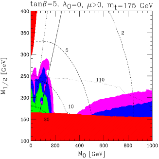
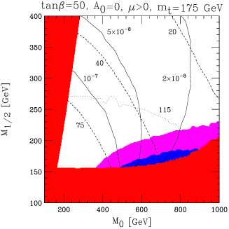
Figure 19: Regions of the $m_{0},m_{1/2}$ plane where the trilepton events should be detectable at the level of $5\sigma$ significance for $\tan\beta=5$ (left) and $\tan\beta=50$ (right) [48]. Three areas are shown for the integrated luminosity of 30 fb^-1 (magenda), 10 fb^-1 (blue) and 2 fb^-1 (green). The large red regions are excluded. Dashed lines represent the SUSY contribution to the muon anomalous magnetic moment (in units of $10^{-10}$) and the dotted lines are iso-mass contours of the lightest neutral Higgs boson.

In the trilepton channel the Tevatron will be sensitive up to $m_{1/2}\leq 250$ GeV if $m_{0}\ \leq 200$ GeV and up to $m_{1/2}\leq 200$ GeV if $m_{0}\ \geq 500$ GeV.

LHC

The LHC hadron collider is the ultimate machine for new physics at the TeV scale. Its c.m. energy is planned to be 14 TeV with very high luminosity up to a few hundred fb^-1. The LHC is supposed to cover A wide range of parameters of the MSSM (see Figs. below) and discover the superpartners with the masses below 2 TeV [50]. This will be a crucial test for the MSSM and the low energy supersymmetry. The LHC potential to discover supersymmetry is widely discussed in the literature [50]-[52].

The gluino and squark production cross sections at LHC can reach 1 pb for masses around 1 TeV. Their decays produce missing transverse momentum from the LSP escape plus multiple jets and a varying number of leptons from the intermediate gauginos. The main decay mode is quarks and gluons plus the LSP. Cascade decays and as a consequence of multilepton events are almost negligible. A typical event with the cascade squark decay is shown in Fig.20.

Figure 20: The cascade decay of squarks into jets and neutralino with possible addition of multileptons

The LHC will be able to discover SUSY with squark and gluino masses up to $2\div 2.5$ TeV for the luminosity $L_{tot}=100\ fb^{-1}$. The expected discovery reach for various channels is shown in Figs.21, 22. The most powerful signature for squark and gluino detection are multijet events; however, the discovery potential depends on relation between the LSP, squark, and gluino masses, and decreases with the increase of the LSP mass.

Figure 21: Expected sparticle reach in various channels at LHC [51]

Figure 22: Expected squarks and gluino reach at LHC for various luminosities [51]

Figure 23: Expected slepton reach at LHC [51]

Slepton pairs produced through the Drell-Yan mechanism $pp\to\gamma^{*}/Z^{*}\to\tilde{l}^{+}\tilde{l}^{-}$ can be detected through their leptonic decays $\tilde{l}\to l+\tilde{\chi}^{0}_{1}$. The typical signature used for sleptons detection is the dilepton pair with missing energy and no hadronic jets. For the luminosity $L_{tot}=100\ fb^{-1}$ LHC will be able to discover sleptons with the masses up to 400 GeV [50]. The discovery reach for sleptons in various channels is shown in Fig.23.

Chargino and neutralino pairs are also produced via the Drell-Yan mechanism $pp\to\tilde{\chi}^{\pm}_{1}\tilde{\chi}^{0}_{2}$ and may be detected through their leptonic decays $\tilde{\chi}^{\pm}_{1}\tilde{\chi}^{0}_{2}\to lll+E_{T}^{miss}$. So their main signature is the isolated leptons with missing energy. The main background to the three lepton channel comes from $WZ/ZZ,t\bar{t},Zb\bar{b}$ and $b\bar{b}$ production. There could also be SUSY background arising from squarks and gluino cascade decays into multileptonic modes. In the case of light gauginos and heavy squarks and sleptons, which can be realized in some regions of parameter space of the MSSM, the cross sections for gaugino production may exceed those of strongly interacting particles. Neutralinos and charginos could be detected provided their masses are lighter than 350 GeV [50].

1.9 Conclusion

Supersymmetry is now the most popular extension of the Standard Model. It promises us that new physics is round the corner at a TeV scale to be exploited at new machines of this decade. If our expectations are correct, very soon we will face new discoveries, the whole world of supersymmetric particles will show up and the table of fundamental particles will be enlarged in increasing rate. This would be a great step in understanding the microworld.

2 PART II    EXTRA DIMENSIONS

2.1 The main ideas

Extra dimensions attracted considerable interest in recent years mainly due to unusual possibilities and intriguing effects even in classical physics. (For review see, e.g. Refs.[53]. We follow mostly Yu.Kubyshin paper.) There is no much motivation for ED in particle physics except for the string theory paradigm. The point is that to be consistent the string theory requires cancellation of conformal anomaly which is possible in the critical dimension equal to 26 for the bosonic string and 10 for the fermionic one [54]. This way the ED come into play. Due to the presence of entirely new ingredients these models provide solutions to some problems of the SM, in particular, of the hierarchy problem in GUTs.

To explain why we do not see the ED, one usually refers to the so-called Kaluza-Klein picture [55]. It is believed that the space-time has 3 large spacial dimensions, and small and compact extra ones. We do not see them because the radius of ED is too small for the present energies, say, equal to the Planck length, $10^{-33}$ cm. This is shown symbolically in Fig.24.

Figure 24: Two possible constructions of the Extra dimensions

At the same time, recently there appeared an alternative explanation. This one is related to the so-called brane-world picture [56, 57]. Here we do not assume small and compact ED, but rather large ones, and the reason why we do not see them is that we are ”localized” on a 4-dimensional brane in this multidimensional space-time (see Fig.24). This is similar to being confined in a potential well and not being able to escape it if the energy is not big enough. To get an example of such a localization, consider some classical solution of the form of a kink [58]. Its energy is localized in the transition region and the corresponding particle seems to be localized in this region (see Fig.25).

Figure 25: The simplest localization: the kink solution and its energy density

Both the pictures or even some combination of them may well be realized in Nature and below we consider some consequences of such an assumption.

2.2 Kaluza-Klein Approach

The KK approach is based on the hypothesis that the space-time is a (4+d)-dimensional pseudo Euclidean space [59]

$$E_{4+d}=M_{4}\times K_{d},$$

where $M_{4}$ is the four-dimensional space-time and $K_{d}$ is $d$-dimensional compact space of characteristic size (scale) $R$. In accordance with the direct product structure of the space-time, the metric is usually chosen to be

$$ds^{2}=\hat{G}_{MN}(\hat{x})d\hat{x}^{M}d\hat{x}^{N}=g_{\mu\nu}(x)dx^{\mu}dx^{\nu}+\gamma_{mn}(x,y)dy^{m}dy^{n}.$$ (2.1)

To interpret the theory as an effective four-dimensional one, the field $\hat{\phi}(x,y)$ depending on both coordinates is expanded in a Fourier series over the compact space

$$\hat{\phi}(x,y)=\sum_{n}\phi^{(n)}(x)Y_{n}(y),$$ (2.2)

where $Y_{n}(y)$ are orthogonal normalized eigenfunctions of the Laplace operator $\Delta_{K_{d}}$ on the internal space $K_{d}$,

$$\Delta_{K_{d}}Y_{n}(y)=\frac{\lambda_{n}}{R^{2}}Y_{n}(y).$$ (2.3)

The coefficients $\phi^{(n)}(x)$ of the Fourier expansion (2.2) are called the Kaluza-Klein modes and play the role of fields of the effective four-dimensional theory. Their masses are given by

$$m_{n}^{2}=m^{2}+\frac{\lambda_{n}}{R^{2}},$$ (2.4)

where $R$ is the radius of the compact dimension.

The coupling constant $g_{(4)}$ of the 4-dimensional theory is related to the coupling constant $g_{(4+d)}$ of the initial (4+d)-dimensional one by

$$g_{(4)}=\frac{g_{(4+d)}}{V_{(d)}},$$ (2.5)

$V_{(d)}\propto R^{d}$ being the volume of the space of extra dimensions.

2.2.1 Low scale gravity

Consider now the Einstein $(4+d)$-dimensional gravity with the action

$$S_{E}=\int d^{4+d}\hat{x}\sqrt{-\hat{G}}\frac{1}{16\pi G_{N(4+d)}}{\cal R}^{(4+d)}[\hat{G}_{MN}],$$

where the scalar curvature ${\cal R}^{(4+d)}[\hat{G}_{MN}]$ is calculated using the metric $\hat{G}_{MN}$. Performing the mode expansion and integrating over $K_{d}$ one arrives at the four-dimensional action

$$S_{E}=\int d^{4}x\sqrt{-g}\left\{\frac{1}{16\pi G_{N(4)}}{\cal R}^{(4)}[g^{(0)}_{MN}]+\mbox{non-zero KK modes}\right\},$$

Similar to eq.(2.5), the relation between the 4-dimensional and $(4+d)$-dimensional gravitational (Newton) constants is given by

$$G_{N(4)}=\frac{1}{V_{(d)}}G_{N(4+d)}.$$ (2.6)

One can rewrite this relation in terms of the 4-dimensional Planck mass $M_{Pl}=(G_{N(4)})^{-1/2}=1.2\cdot 10^{19}\;\mbox{GeV}$ and a fundamental mass scale of the $(4+d)$-dimensional theory $M\equiv(G_{N(4+d)})^{-\frac{1}{d+2}}$. One gets

$$M_{Pl}^{2}=V_{(d)}M^{d+2}.$$ (2.7)

This formula is often referred to as the reduction formula.

Thus, the fundamental scale of a multidimensional theory becomes $M$ rather than $M_{Pl}$. This way the problem of hierarchy is reduced to a less severe one in extra dimensions. The scale $M$ is not restricted by experimental value of the Newtonian constant and may take values $\sim$ few TeV. Assuming $M=1\ TeV$ one can rewrite eq.(2.7) as [56]

$$R\sim\frac{1}{M}\left(\frac{M_{Pl}}{M}\right)^{2/d}\sim 10^{\frac{30}{d}-17}\;\mbox{cm},$$ (2.8)

or

$$R^{-1}\sim M\left(\frac{M}{M_{Pl}}\right)^{2/d}\sim 10^{-\frac{30}{d}+3}\;\mbox{GeV}.$$ (2.9)

Let us analyze various cases. In the case $d=1$ it follows from eq.(2.8) that $R\sim 10^{13}\mbox{cm}$, i.e. the size of extra dimensions is of the order of the solar distance. This case is obviously excluded. For $d\geq 2$ we obtain:

for   $d=2$	$R\sim 0.1\;\mbox{mm}$,	$R^{-1}\sim 10^{-3}\;\mbox{eV}$
for   $d=3$	$R\sim 10^{-7}\;\mbox{cm}$,	$R^{-1}\sim 100\;\mbox{eV}$
$\ldots$	$\ldots$	$\ldots$
for   $d=6$	$R\sim 10^{-12}\;\mbox{cm}$,	$R^{-1}\sim 10\;\mbox{MeV}$

Such sizes of extra dimensions are already acceptable because no deviations from the Newtonian gravity have been observed for distances $r\sim 1$ mm so far (see, for example, [60]). On the other hand, the SM has been accurately checked already at the scale $\sim 100$ GeV. To overcome this difficulty it is supposed [56] that the SM fields are localized on the 4d brane while only gravitons propagate in the bulk.

At the same time, these conclusions strongly depend on the choice of the scale M. If one takes bigger scale, the corresponding radius decreases very fast (see Fig.26).

Figure 26: The dependence of the radius of compactification $R$ on the multidimensional fundamental scale $M$ for $d=6$

The presence of ED leads to the modification of classical gravity. The Newton potential between two test masses $m_{1}$ and $m_{2}$, separated by a distance $r$, is in this case equal to

$$V(r)=G_{N(4)}m_{1}m_{2}\sum_{n}\frac{1}{r}e^{-m_{n}r}=G_{N(4)}m_{1}m_{2}\left(\frac{1}{r}+\sum_{n\neq 0}\frac{1}{r}e^{-|n|r/R}\right).$$

The first term in the last bracket is the contribution of the usual massless graviton (zero mode) and the second term is the contribution of the massive gravitons. For the size $R$ large enough (i.e. for the spacing between the modes small enough) this sum can be replaced by the integral and one gets [56]

$$V(r) = G_{N(4)}\frac{m_{1}m_{2}}{r}\left[1+S_{d-1}\int_{1/R}^{\infty}e^{-mr}m^{d-1}dm\right]$$ (2.10)

$$= G_{N(4)}\frac{m_{1}m_{2}}{r}\left[1+S_{d-1}\left(\frac{R}{r}\right)^{d}\int_{r/R}^{\infty}e^{-z}z^{d-1}dz\right],$$

where $S_{d-1}$ is the area of the $(d-1)$-dimensional sphere of the unit radius. This leads to the following behaviour of the potential at short and long distances

$$V\approx\left\{\begin{array}[]{ll}G_{N(4)}\frac{\displaystyle m_{1}m_{2}}{\displaystyle r}&r\gg R,\\ G_{N(4)}\frac{\displaystyle m_{1}m_{2}}{\displaystyle r}S_{d-1}\left(\frac{\displaystyle R}{\displaystyle r}\right)^{d}\Gamma(d)=G_{N(4+d)}\frac{\displaystyle m_{1}m_{2}}{\displaystyle r^{d+1}}S_{d-1}\Gamma(d)&r\ll R,\end{array}\right.$$ (2.11)

Thus, one has a modification of classical gravity at small distances which may have observational consequences.

2.2.2 The ADD model

The ADD model was proposed by N. Arkani-Hamed, S. Dimopoulos and G. Dvali in Ref. [56]. The model includes the SM localized on a 3-brane embedded into the $(4+d)$-dimensional space-time with compact extra dimensions. The gravitational field is the only field which propagates in the bulk.

To analyze the field content of the effective (dimensionally reduced) four-dimensional model, consider the field $\hat{h}_{MN}(x,y)$ describing the linear deviation of the metric around the $(4+d)$-dimensional Minkowski background $\eta_{MN}$

$$\hat{G}_{MN}(x,y)=\eta_{MN}+\frac{2}{M^{1+d/2}}\hat{h}_{MN}(x,y)$$ (2.12)

Let us assume, for simplicity, that the space of extra dimensions is the $d$-dimensional torus. Performing the KK mode expansion

$$\hat{h}_{MN}(x,y)=\sum_{n}h^{(n)}_{MN}(x)\frac{1}{\sqrt{V_{(d)}}}\exp(-i\frac{n_{m}y^{m}}{R}),$$ (2.13)

where $V_{(d)}$ is the volume of the space of extra dimensions, we obtain the KK tower of states $h^{(n)}_{MN}(x)$ with masses

$$m_{n}=\frac{1}{R}\sqrt{n_{1}^{2}+n_{2}^{2}+\ldots+n_{d}^{2}}\equiv\frac{|n|}{R},$$ (2.14)

so that the mass splitting is $\Delta m\propto 1/R.$

The interaction of the KK modes $h^{(n)}_{MN}(x)$ with fields on the brane is determined by the universal minimal coupling of the $(4+d)$-dimensional theory

$$S_{int}=\int d^{4+d}\hat{x}\sqrt{-\hat{G}}\hat{T}_{MN}\hat{h}^{MN}(x,y),$$

where the energy-momentum tensor of the matter localized on the brane at $y=0$ has the form

$$\hat{T}_{MN}(x,y)=\delta_{M}^{\mu}\delta_{N}^{\nu}T_{\mu\nu}(x)\delta^{(d)}(y).$$

Using the reduction formula (2.7) and the KK expansion (2.13) one obtains that

$$S_{int}=\int d^{4}xT_{\mu\nu}\sum_{n}\frac{1}{M^{1+d/2}\sqrt{V_{(d)}}}h^{(n)\mu\nu}(x)=\sum_{n}\int d^{4}x\frac{1}{M_{Pl}}T^{\mu\nu}(x)h^{(n)}_{\mu\nu}(x),$$ (2.15)

which is the usual interaction of matter with gravity suppressed by $M_{Pl}$.

The degrees of freedom of the four-dimensional theory, which emerge from the multidimensional metric, include [61, 62]

1. the massless graviton and the massive KK gravitons $h^{(n)}_{\mu\nu}$ (spin-2 fields) with masses given by eq.(2.14);

2. $(d-1)$ KK towers of spin-1 fields which do not couple to $T_{\mu\nu}$;

3. $(d^{2}-d-2)/2$ KK towers of real scalar fields (for $d\geq 2$), they do not couple to $T_{\mu\nu}$ either;

4. a KK tower of scalar fields coupled to the trace of the energy-momentum tensor $T_{\mu}^{\mu}$, its zero mode is called radion and describes fluctuations of the volume of extra dimensions.

Alternatively, one can consider the $(4+d)$-dimensional theory with the $(4+d)$-dimensional massless graviton $\hat{h}_{MN}(x,y)$ interacting with the SM fields with couplings $\sim 1/M^{1+d/2}$.

In the 4-dimensional picture the coupling of each individual graviton (both massless and massive) to the SM fields is small $\sim 1/M_{Pl}$. However, the smallness of the coupling constant is compensated by the high multiplicity of states with the same mass. Indeed, the number $d{\cal N}(|n|)$ of modes with the modulus $|n|$ of the quantum number being in the interval $(|n|,|n|+d|n|)$ is equal to

$$d{\cal N}(|n|)=S_{d-1}|n|^{d-1}d|n|=S_{d-1}R^{d}m^{d-1}dm\sim S_{d-1}\frac{M_{Pl}}{M^{d+2}}m^{d-1}dm,$$ (2.16)

where we used the mass formula $m=|n|/R$ and the reduction formula (2.7). The number of KK gravitons $h^{(n)}$ with masses $m_{n}\leq E<M$ is equal to

$${\cal N}(E)\sim\int_{0}^{ER}d{\cal N}(|n|)\sim S_{d-1}\frac{M^{2}_{Pl}}{M^{d+2}}\int_{0}^{E}m^{d-1}dm=\frac{S_{d-1}}{d}\frac{M^{2}_{Pl}}{M^{d+2}}E^{d}\sim R^{d}E^{d}.$$

One can see that for $E\gg R^{-1}$ the multiplicity of states which can be produced is large. Hence, despite the fact that due to eq.(2.15) the amplitude of emission of the mode $n$ is ${\cal A}\sim 1/M_{Pl}$, the total combined rate of emission of the KK gravitons with masses $m_{n}\leq E$ is

$$\sim\frac{1}{M_{Pl}^{2}}{\cal N}(E)\sim\frac{E^{d}}{M^{d+2}}.$$ (2.17)

We can see that there is a considerable enhancement of the effective coupling due to the large phase space of KK modes or due to the large volume of the space of extra dimensions. Because of this enhancement the cross-sections of processes involving the production of KK gravitons may turn out to be quite noticeable at future colliders.

2.2.3 HEP phenomenology

There are two types of processes at high energies in which the effect of the KK modes of the graviton can be observed at running or planned experiments. These are the graviton emission and virtual graviton exchange processes [61]-[65].

We start with the graviton emission, i.e., the reactions where the KK gravitons are created as final state particles. These particles escape from the detector, so that a characteristic signature of such processes is missing energy. Though the rate of production of each individual mode is suppressed by the Planck mass, due to the high multiplicity of KK states the magnitude of the total rate of production is determined by the TeV scale (see eq.(2.17)). Taking eq.(2.16) into account, the relevant differential cross section [61] is

$$\frac{d^{2}\sigma}{dtdm}\sim S_{d-1}\frac{M^{2}_{Pl}}{M^{d+2}}m^{d-1}\frac{d\sigma_{m}}{dt}\sim\frac{1}{M^{d+2}},$$ (2.18)

where $d\sigma_{m}/dt$ is the differential cross section of the production of a single KK mode with mass $m$.

At $e^{+}e^{-}$ colliders the main contribution comes from the $e^{+}e^{-}\rightarrow\gamma h^{(n)}$ process. The main background comes from the process $e^{+}e^{-}\rightarrow\nu\bar{\nu}\gamma$ and can be effectively suppressed by using polarized beams. Figure 27 shows the total cross section of the graviton production in electron-positron collisions [65]. To the right is the same cross section as a function of $M$ for $\sqrt{s}=800\;\mbox{GeV}$ [66].

Figure 27: The total cross sections for $e^{+}e^{-}\rightarrow\gamma\nu_{i}\bar{\nu}_{i}$ ($i=e,\mu,\tau$) and $e^{+}e^{-}\rightarrow\gamma h$ (faster growing curves) for $d=2$ and $M=2.5$ TeV [65] (left) and the cross section for $e^{+}e^{-}\rightarrow\gamma h^{(n)}$ at $\sqrt{s}=800$ GeV as a function of the scale $M$ for A different number $\delta$ of extra dimensions (right). Horizontal lines indicate the background. [66]

Effects due to gravitons can also be observed at hadron colliders. A characteristic process at the LHC would be $pp\rightarrow(\mbox{jet}+\mbox{missing}\;E)$. The subprocess that gives the largest contribution is the quark-gluon collision $qg\rightarrow qh^{(n)}$. Other subprocesses are $q\bar{q}\rightarrow gh^{(n)}$ and $gg\rightarrow gh^{(n)}$.

Processes of another type, in which the effects of extra dimensions can be observed, are exchanges of virtual KK modes, in particular, the virtual graviton exchanges. Contributions to the cross section from these additional channels lead to deviation from the behaviour expected in the 4-dimensional model. An example is $e^{+}e^{-}\rightarrow f\bar{f}$ with $h^{(n)}$ being the intermediate state (see Fig.28). Moreover, gravitons can mediate processes absent in the SM at the tree-level, for example, $e^{+}e^{-}\rightarrow HH$, $e^{+}e^{-}\rightarrow gg$. Detection of such events with large cross sections may serve as an indication of the existence of extra dimensions.

Figure 28: The Feynman diagram for the virtual graviton exchange (left) and deviation from the expectations of the SM (histogram) for Bhabha scattering at a $500\;\mbox{GeV}$ $e^{+}e^{-}$ collider for the Left-Right polarization asymmetry as a function of $z=\cos\theta$ for $M=1.5\;\mbox{TeV}$ and the integrated luminosity ${\cal L}=75\;\mbox{fb}^{-1}$ (right) [64].

The $s$-channel amplitude of a graviton-mediated scattering process is given by

$${\cal A}=\frac{1}{M_{Pl}^{2}}\sum_{n}\left\{T_{\mu\nu}\frac{P^{\mu\nu}P^{\rho\sigma}}{s-m_{n}^{2}}T_{\rho\sigma}+\sqrt{\frac{3(d-1)}{d+2}}\frac{T^{\mu}_{\mu}T^{\nu}_{\nu}}{s-m_{n}^{2}}\right\},$$ (2.19)

where $P_{\mu\nu}$ is a polarization factor coming from the propagator of the massive graviton and $T_{\mu\nu}$ is the energy-momentum tensor [61]. It contains a kinematic factor

$${\cal S} = \frac{1}{M_{Pl}^{2}}\sum_{n}\frac{1}{s-m_{n}^{2}}\approx\frac{1}{M_{Pl}^{2}}S_{d-1}\frac{M_{Pl}^{2}}{M^{d+2}}\int^{\Lambda}\frac{m^{d-1}dm}{s-m^{2}}$$ (2.20)

$$= \frac{S_{d-1}}{2M^{4}}\left\{i\pi\left(\frac{s}{M^{2}}\right)^{d/2-1}+\sum_{k=1}^{[(d-1)/2]}c_{k}\left(\frac{s}{M^{2}}\right)^{k-1}\left(\frac{\Lambda}{M}\right)^{d-2k}\right\}.$$

Since the integrals are divergent for $d\geq 2$, the cutoff $\Lambda$ was introduced. It sets the limit of applicability of the effective theory. Because of the cutoff,the amplitude cannot be calculated explicitly without the knowledge of a full fundamental theory. Usually, in the literature it is assumed that the amplitude is dominated by the lowest-dimensional local operator (see [61]).

The characteristic feature of expression (2.20) different from the 4-dimensional model is the increase of the cross section with energy. This is a consequence of the exchange of the infinite tower of the KK modes. Note, however, that this result is based on a tree-level amplitude, while the radiative corrections in this case are power-like and may well change this behaviour.

Typical processes, in which the virtual exchange via massive gravitons can be observed, are: (a) $e^{+}e^{-}\rightarrow\gamma\gamma$; (b) $e^{+}e^{-}\rightarrow f\bar{f}$, for example the Bhabha scattering $e^{+}e^{-}\rightarrow e^{+}e^{-}$ or Möller scattering $e^{-}e^{-}\rightarrow e^{-}e^{-}$; (c) graviton exchange contribution to the Drell-Yang production. A signal of the KK graviton mediated processes is the deviation in the number of events and in the left-right polarization asymmetry from those predicted by the SM (see Figs. 28) [64].

2.3 Brane-World Models

2.3.1 The Randal-Sundram model

The RS model [57] is a model of Einstein gravity in five-dimensional Anti-de Sitter space-time with extra dimension being compactified to the orbifold $S^{1}/Z_{2}$. There are two 3-branes in the model located at the fixed points $y=0$ and $y=\pi R$ of the orbifold, where $R$ is the radius of the circle $S^{1}$. The brane at $y=0$ is usually referred to as A Planck brane, whereas the brane at $y=\pi R$ is called A TeV brane (see Fig.29). The SM fields are constrained to the TeV brane, while gravity propagates in the additional dimension.

Figure 29: The Randall-Sundrum construction of the extra-dimensional space

The action of the model is given by

$$S = \int d^{4}x\int_{-\pi R}^{\pi R}dy\sqrt{-\hat{G}}\left\{2M^{3}{\cal R}^{(5)}\left[\hat{G}_{MN}\right]+\Lambda\right\}$$ (2.21)

$$+ \int_{B_{1}}d^{4}x\sqrt{-g^{(1)}}\left(L_{1}-\tau_{1}\right)+\int_{B_{2}}d^{4}x\sqrt{-g^{(2)}}\left(L_{2}-\tau_{2}\right),$$

where ${\cal R}^{(5)}$ is the five-dimensional scalar curvature, $M$ is a mass scale (the five-dimensional ”Planck mass”) and $\Lambda$ is the cosmological constant. $L_{j}$ is a matter Lagrangian and $\tau_{j}$ is a constant vacuum energy on brane $j$ $(j=1,2)$.

The RS solution describes the space-time with non factorizable geometry with the metric given by

$$ds^{2}=e^{-2\sigma(y)}\eta_{\mu\nu}dx^{\mu}dx^{\nu}+dy^{2}.$$ (2.22)

The additional coordinate changes inside the interval $-\pi R<y\leq\pi R$ and the function $\sigma(y)$ in the warp factor $\exp(-2\sigma)$ is equal to

$$\sigma(y)=k|y|,\;\;\;(k>0).$$ (2.23)

For the solution to exist the parameters must be fine-tuned to satisfy the relations

$$\tau_{1}=-\tau_{2}=24M^{3}k,\;\;\;\Lambda=24M^{3}k^{2}.$$

Here $k$ is a dimensional parameter which was introduced for convenience. This fine-tuning is equivalent to the usual cosmological constant problem. If $k>0$, then the tension on brane 1 is positive, whereas the tension $\tau_{2}$ on brane 2 is negative.

For a certain choice of the gauge the most general perturbed metric is given by

$$ds^{2}=e^{-2k|y|}\left(\eta_{\mu\nu}+\tilde{h}_{\mu\nu}(x,y)\right)dx^{\mu}dx^{\nu}+(1+\phi(x))dy^{2}.$$

and describes the graviton field $\tilde{h}_{\mu\nu}(x,y)$ and the radion field $\phi(x)$ [67].

As a next step the field $h_{\mu\nu}(x,y)$ is decomposed over an appropriate system of orthogonal and normalized functions:

$$h_{\mu\nu}(x,y)=\sum_{n=0}^{\infty}h_{\mu\nu}^{(n)}(x)\frac{\chi_{n}(y)}{R}.$$ (2.24)

The particles localized on the branes are:

Brane 1 (Planck):

• massless graviton $h_{\mu\nu}^{(0)}(x)$,

• massive KK gravitons $h_{\mu\nu}^{(n)}(x)$ with masses $m_{n}=\beta_{n}ke^{-\pi kR}$, where $\beta_{n}=3.83,7.02,10.17,13.32,\ldots$ are the roots of the Bessel function,

• massless radion $\phi(x)$.

Brane 2 (TeV):

• massless graviton $h_{\mu\nu}^{(0)}(x)$,

• massive KK gravitons $h_{\mu\nu}^{(n)}(x)$ with masses $m_{n}=\beta_{n}k$,

• massless radion $\phi(x)$.

The brane 2 is most interesting from the point of view of high energy physics phenomenology. Because of the nontrivial warp factor $e^{-2\sigma(\pi R)}$, the Planck mass here is related to the fundamental 5-dimensional scale $M$ by

$$M_{Pl}^{2}=e^{2k\pi R}\int_{-\pi R}^{\pi R}dye^{-2k|y|}=\frac{M^{3}}{k}\left(e^{2k\pi R}-1\right).$$ (2.25)

This way one obtains the solution of the hierarchy problem. The large value of the 4-dimensional Planck mass is explained by an exponential wrap factor of geometrical origin, while the scale $M$ stays small.

The general form of the interaction of the fields, emerging from the five-dimensional metric, with the matter localized on the branes is given by the expression:

$$\frac{1}{2M^{3/2}}\int_{B_{1}}d^{4}x\ h_{\mu\nu}(x,0)T^{(1)}_{\mu\nu}+\frac{1}{2M^{3/2}}\int_{B_{2}}d^{4}x\ h_{\mu\nu}(x,0)T^{(2)}_{\mu\nu}\sqrt{-\det\gamma_{\mu\nu}(\pi R)}$$

Decomposing the field $h_{\mu\nu}(x,y)$ according to (2.24) the interaction Lagrangian can be written as

$$\frac{1}{2}\int_{B_{2}}d^{4}z\left[\frac{1}{M_{Pl}}h^{(0)}_{\mu\nu}(z)T^{(2)\mu\nu}-\sum_{n=1}^{\infty}\frac{w_{n}}{\Lambda_{\pi}}h^{(n)}_{\mu\nu}T^{(2)\mu\nu}-\frac{1}{\Lambda_{\pi}\sqrt{3}}T^{(2)\mu}_{\mu}\right],$$ (2.26)

where $\Lambda_{\pi}=M_{Pl}e^{-k\pi R}\approx\sqrt{M^{3}/k}$ and $M_{Pl}$ is given by eq.(2.25) .

The massless graviton, as in the standard gravity, interacts with matter with the coupling $M_{Pl}^{-1}$. The interaction of the massive gravitons and radion are considerably stronger: their couplings are $\propto\Lambda_{\pi}^{-1}\sim 1\;\mbox{TeV}^{-1}$. If a few first massive KK gravitons have masses $M_{n}\sim 1$TeV, then this leads to new effects which in principle can be seen at future colliders. To have this situation, the fundamental mass scale $M$ and the parameter $k$ are taken to be $M\sim k\sim 1$TeV.

2.3.2 HEP phenomenology

With the mass of the first KK mode $M_{1}\sim 1\;\mbox{TeV}$ direct searches for the first KK graviton $h^{(1)}$ in the resonance production at future colliders become quite possible. Signals of the graviton detection can be [68]

$\bullet$ an excess in the Drell-Yan processes     $\begin{array}[]{l}\\ q\bar{q}\rightarrow h^{(1)}\rightarrow l^{+}l^{-},\\ gg\rightarrow h^{(1)}\rightarrow l^{+}l^{-}\end{array}$

$\bullet$ an excess in the dijet channel               $q\bar{q},gg\rightarrow h^{(1)}\rightarrow q\bar{q},gg.$

The plots of the exclusion regions for the Tevatron and LHC [68] are presented in Fig. 30.

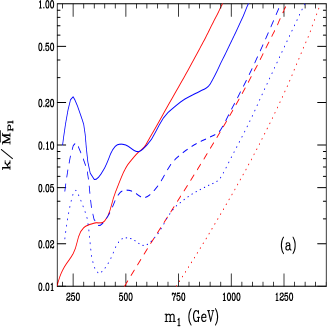
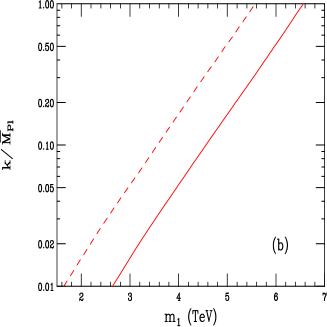
Figure 30: Exclusion region for resonance production of the first KK graviton excitation in the Drell-Yan (corresponding to the diagonal lines) and dijet (represented by the bumpy curves) channels at the Tevatron (left). The solid curves represent the results for Run I, while the dashed and dotted curves correspond to Run II with 2, 30 fb^-1 of integrated luminosity, respectively. The same for the LHC (right). The dashed, solid curves correspond to 10, 100 fb^-1 of integrated luminosity, respectively.

They show the exclusion region for resonance production of the first KK graviton excitation in the Drell-Yan and dijet channels. The excluded region lies above and to the left of the curves.

The next plots present the behaviour of the cross-section of the Drell-Yan process as a function of the invariant mass of the final leptons. It is shown for two values of $M_{1}$ for the cases of the Tevatron and the LHC in Fig. 31. One can see the characteristic peaks in the cross section for one or a series of massive graviton modes.

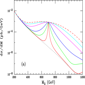
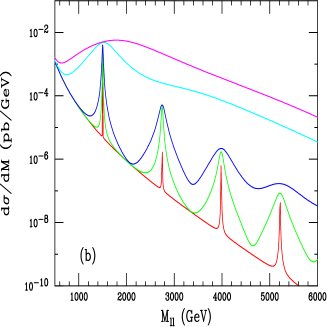
Figure 31: Drell-Yan production of the KK graviton with $M_{1}=700$ GeV at the Tevatron (left) and for the LHC (right) for $M_{1}=1500$ GeV and its subsequent tower states [68].

The possibility to detect the resonance production of the first massive graviton in the proton - proton collisions $pp\rightarrow h^{(1)}\rightarrow e^{+}e^{-}$ at the LHC depends on the cross section. The main background processes are $pp\rightarrow Z/\gamma^{*}\rightarrow e^{+}e^{-}$. The estimated cross section of the process $h^{(1)}\rightarrow e^{+}e^{-}$ as a function of $M_{1}$ in the RS model is shown in Fig. 32 [69]. One can see that the detection might be possible if $M_{1}\leq 2080\;\mbox{GeV}$ .

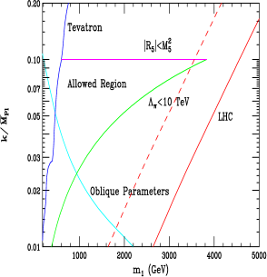
Figure 32: The cross-section times branching ratio, $\sigma\cdot B$, for $h^{(1)}\rightarrow e^{+}e^{-}$ in the RS model and the smallest detectable cross-section times the branching ratio, $(\sigma\cdot B)^{min}$ [69] (left) and the summary of experimental and theoretical constraints on the parameters $M_{1}$ and $\eta=(k/M_{Pl})e^{k\pi R}$ (right) [68]. The allowed region lies as indicated. The LHC sensitivity to graviton resonances in the Drell-Yan channel is represented by diagonal dashed and solid curves, corresponding to 10 and 100 fb^-1 of integrated luminosity, respectively

To be able to conclude that the observed resonance is a graviton and not, for example, a spin-1 $Z^{\prime}$ resonance or a similar particle, it is necessary to check that it is produced by a spin-2 intermediate state. The spin of the intermediate state can be determined from the analysis of the angular distribution function $f(\theta)$ of the process, where $\theta$ is the angle between the initial and final beams. This function is

$$Spin\ 0 => f(\theta)=1,$$

$$Spin\ 1 => f(\theta)=1+\cos^{2}\theta,$$

$$Spin\ 2 => \left\{\begin{array}[]{ll}q\bar{q}\rightarrow h^{(1)}\rightarrow e^{+}e^{-}&f(\theta)=1-3\cos^{2}\theta+4\cos^{4}\theta,\\ gg\rightarrow h^{(1)}\rightarrow e^{+}e^{-}&f(\theta)=1-\cos^{4}\theta.\end{array}\right.$$

The analysis, carried out in Ref. [69], shows that angular distributions allow one to determine the spin of the intermediate state with 90% C.L. for $M_{1}\leq 1720$ GeV.

As a next step it would be important to check the universality of the coupling of the first massive graviton $h^{(1)}$ by studying various processes, e.g. $pp\rightarrow h^{(1)}\rightarrow l^{+}l^{-},\;\mbox{jets},\;\gamma\gamma,W^{+}W^{-},HH$, etc. If it is kinematically feasible to produce higher KK modes, measuring the spacings of the spectrum will be another strong indication in favour of the RS model.

The conclusion is [68] that with the integrated luminosity ${\cal L}=100\;\mbox{fb}^{-1}$ the LHC will be able to cover the natural region of parameters $(M_{1},\eta=(k/M_{Pl})e^{k\pi R})$ and, therefore, discover or exclude the RS model. This is illustrated in the r.h.s. of Fig. 32.

2.4 Conclusion

We finish with a short summary of the main features of the ADD and RS models.

ADD Model.

1. The ADD model removes the $M_{EW}/M_{Pl}$ hierarchy, but replaces it by the hierarchy

   $$\frac{R^{-1}}{M}\sim\left(\frac{M}{M_{Pl}}\right)^{2/d}\sim 10^{-\frac{30}{d}}.$$

   For $d=2$ this relation gives $R^{-1}/M\sim 10^{-15}$. This hierarchy is of different type and might be easier to understand or explain, perhaps with no need for SUSY;

2. The model predicts the modification of the Newton law at short distances which may be checked in precision experiments;

3. For $M$ small enough high-energy physics effects, predicted by the model, can be discovered at future collider experiments.

RS model

1. The model solves the $M_{EW}/M_{Pl}$ hierarchy problem without generating a new hierarchy.

2. A large part of the allowed range of parameters of the RS model will be studied in future collider experiments which will either discover new phenomena or exclude the most ”natural” region of its parameter space.

3. With a mechanism of radion stabilization added the model is quite viable. In this case, cosmological scenarios, based on the RS model, are consistent without additional fine-tuning of parameters (except the cosmological constant problem) [70].

Acknowledgements

I am grateful to the organizers of the School at Sant-Feliu for providing very nice atmosphere during the school and to the students for their interest, patience, and attention. Financial support from RFBR grant # 99-02-16650, the grant of THE Russian Ministry of Industry, Science and Technologies # 2339.2003.2 is kindly acknowledged. I would like to thank the Theory Group of KEK, where this manuscript was finished, for support and hospitality.

References

• [1] P. Fayet and S. Ferrara, Phys. Rep. 32 (1977) 249; M. F. Sohnius, Phys. Rep. 128 (1985) 41; H. P. Nilles, Phys. Rep. 110 (1984) 1; H. E. Haber and G. L. Kane, Phys. Rep. 117 (1985) 75; A. B. Lahanas and D. V. Nanopoulos, Phys. Rep. 145 (1987) 1.
• [2] J. Wess and J. Bagger, ”Supersymmetry and Supergravity”, Princeton Univ. Press, 1983.
• [3] S. J. Gates, M. Grisaru, M. Roček and W. Siegel, ”Superspace or One Thousand and One Lessons in Supersymmetry”, Benjamin & Cummings, 1983.
• [4] P.West, Introduction to supersymmetry and supergravity, World Scientific, 2nd edition, 1990.
• [5] S.Weinberg, ”The quantum theory of fields”. Vol. 3, Cambridge, UK: Univ. Press, 2000.
• [6] D. I. Kazakov, ”Beyond the Standard Model (In search of supersymmetry)”, Lectures at the European school on high energy physics, CERN-2001-003, hep-ph/0012288.
• [7] Y. A. Golfand and E. P. Likhtman, JETP Letters 13 (1971) 452; D. V. Volkov and V. P. Akulov, JETP Letters 16 (1972) 621; J. Wess and B. Zumino, Phys. Lett. B49 (1974) 52.
• [8] S. Coleman and J .Mandula, Phys.Rev. 159 (1967) 1251.
• [9] J.Bennett, M.Donahue, N.Schneider, and M.Voit, ”The Cosmic Perspective”, Addison Wesley Pub Co, 2003.
• [10] C.L. Bennett et al., ApJS,bf 148 (2003) 1.
• [11] F. A. Berezin, ”The Method of Second Quantization”, Moscow, Nauka, 1965.
• [12] P. Fayet and J. Illiopoulos, Phys. Lett. B51 (1974) 461.
• [13] L. O’Raifeartaigh, Nucl. Phys. B96 (1975) 331.
• [14] H. E. Haber, ”Introductory Low-Energy Supersymmetry”, Lectures given at TASI 1992, (SCIPP 92/33, 1993), hep-ph/9306207.
• [15] http://atlasinfo.cern.ch/Atlas/documentation/EDUC/physics14.html
• [16] P.Fayet, Nucl. Phys. B90(1975) 104; A.Salam and J.Srathdee, Nucl. Phys. B87(1975) 85.
• [17] H. Dreiner and G. G. Ross, Nucl. Phys. B365 (1991) 597, K. Enqvist, A. Masiero and A. Riotto, Nucl. Phys. B373 (1992) 95,
H. Dreiner and P. Morawitz, Nucl. Phys. B428 (1994) 31; H. Dreiner and H. Pois, preprint NSF-ITP-95-155; hep-ph/9511444,
V. Barger, M. S. Berger , R. J. N. Philips and T. Wöhrmann, Phys. Rev. D53 (1996) 6407.
• [18] L. Hall, J. Lykken and S. Weinberg, Phys. Rev. D27 (1983) 2359; S. K. Soni and H. A. Weldon, Phys. Lett. B126 (1983) 215; I. Affleck, M. Dine and N. Seiberg, Nucl. Phys. B256 (1985) 557.
• [19] H. P. Nilles, Phys. Lett. B115 (1982) 193; A. H. Chamseddine, R. Arnowitt and P. Nath, Phys. Rev. Lett. 49 (1982) 970; Nucl. Phys. B227 (1983) 121; R. Barbieri, S. Ferrara and C. A. Savoy, Phys. Lett. B119 (1982) 343.
• [20] M. Dine and A. E. Nelson, Phys. Rev. D48 (1993) 1277, M. Dine, A. E. Nelson and Y. Shirman, Phys. Rev. D51 (1995) 1362.
• [21] L. Randall and R. Sundrum, Nucl. Phys. B557 (1999) 79; G. F. Giudice, M. A. Luty, H. Murayama and R. Rattazzi, JHEP, 9812 (1998) 027.
• [22] D. E. Kaplan, G. D. Kribs and M. Schmaltz, Phys. Rev. D62 (2000) 035010; Z. Chacko, M. A. Luty, A. E. Nelson and E. Ponton, JHEP, 0001 (2000) 003.
• [23] M. E. Peskin, ”Theoretical summary lecture for EPS HEP99”, hep-ph/0002041.
• [24] G. G. Ross and R. G. Roberts, Nucl. Phys. B377 (1992) 571.
V. Barger, M. S. Berger and P. Ohmann, Phys. Rev. D47 (1993) 1093.
D. M. Pierce, J. A. Bagger, K.T. Matchev, R. Zhang, Nucl.Phys. B491 (1997) 3.
• [25] W. de Boer, R. Ehret and D. Kazakov, Z. Phys. C67 (1995) 647;
W. de Boer et al., Z. Phys. C71 (1996) 415.
• [26] M. Sher, Phys. Lett. B317 (1993) 159; C. Ford, D. R. T. Jones, P. W. Stephenson and M. B. Einhorn, Nucl. Phys. B395 (1993) 17; G. Altarelli and I. Isidori, Phys. Lett. B337 (1994) 141; J. A. Casas, J. R. Espinosa and M. Quiros, Phys. Lett. B342 (1995) 171.
• [27] L. E. Ibáñez, C. Lopéz and C. Muñoz, Nucl. Phys. B256 (1985) 218.
• [28] U. Amaldi, W. de Boer and H. Fürstenau, Phys. Lett. B260 (1991) 447.
• [29] W. Barger, M. Berger, P. Ohman, Phys. Rev. D49 (1994) 4908.
• [30] V.Barger, M.S. Berger, P.Ohmann and R.Phillips, Phys. Lett. B314 (1993) 351.
P. Langacker and N. Polonsky, Phys. Rev. D49 (1994) 1454.
S. Kelley, J. L. Lopez and D.V. Nanopoulos, Phys. Lett. B274 (1992) 387.
• [31] S.Ahmed et al. (CLEO Collaboration), CLEO CONF 99/10, hep-ex/9908022.
• [32] R. Barate et al. (ALEPH Collaboration), Phys. Lett. B429 (1998) 169.
• [33] W.de Boer, M.Huber, C.Sander, D.I.Kazakov, Phys.Lett. B515 (2001) 283.
• [34] ALEPH Collaboration, Phys.Lett. B499 (2001) 67.
• [35] S. Abel et al. [SUGRA Working Group Collaboration], Report of the SUGRA working group for run II of the Tevatron, hep-ph/0003154.
• [36] E.Kolb and M.S.Turner, The Early Universe, Frontiers in Physics, Addison Wesley, 1990.
• [37] G.Jungman, M.Kamionkowski and K.Griest, Phys.Rep. 267 (1996) 195.
• [38] M. Drees and M. M. Nojiri, Phys. Rev. D47 (1993) 376;
J. L. Lopez, D. V. Nanopoulos and H. Pois, Phys. Rev. D47 (1993) 2468;
P. Nath and R. Arnowitt, Phys. Rev. Lett. 70 (1993) 3696.
• [39] W.de Boer and C.Sander, Phys. Lett. B585 (2004) 276.
• [40] W.de Boer, M.Herold, C.Sander, V.Zhukov, hep-ph/0309029.
• [41] W.de Boer, M.Herold, C.Sander, V.Zhukov, A.Gladyshev, and D.Kazakov, astro-ph/0408272.
• [42] S. Heinemeyer, W. Hollik and G. Weiglein, Phys. Lett. B455 (1999) 179; Eur. Phys. J. C9 (1999) 343.
• [43] W.de Boer, M.Huber, A.Gladyshev, D.Kazakov, Eur.Phys.J. C20 (2001) 689.
• [44] D. E. Groom et al., ”Review of Particle Physics”, Eur. Phys. J. C15 (2000) 1.
• [45] M. Masip, R. Muñoz-Tapia and A. Pomarol, Phys. Rev. D57 (1998) 5340.
• [46] CDF Collaboration (D. Acosta et al.), Phys.Rev.Lett. 90 (2003) 251801; CDF Collaboration (T. Affolder et al.), Phys.Rev.Lett. 87 (2003) 251803.
• [47] T.Kamon, hep-ex/0301019, Proc. of IX Int. Conf. ”SUSY-01”, WS 2001, p.196.
• [48] A.Dedes, H.R.Dreiner, U.Nierste, and P.Richardson, hep-ph/0207026.
• [49] M.Carena, D.Choudhury, R.A.Diaz, H.E.Logan, and C.E.M. Wagner, Phys.Rev. D66 (2002) 115010;
E.L.Berger, B.W.Harris, D.E.Kaplan, Z.Sullivan, T.M.P. Tait, and C.E.M. Wagner, Phys.Rev.Lett. 86 (2001) 4231;
R. Culbertson, S.P.Martin, J.Qian, S.Thomas, H.Baer, et al, ”Low-Scale and Gauge-Mediated Supersymmetry Breaking at the Fermilab Tevatron Run II”, hep-ph/0008070;
H.Baer, M.Drees, F.Paige, P.Quintana, X. Tata, Phys.Rev. D61 (2000) 095007;
K.T.Matchev and D.M.Pierce, Phys.Rev. D60 (1999) 075004; Phys.Lett. B467 (1999) 225.
H.Baer, P.G.Mercadante, X.Tata, and Y.Wang,Phys.Rev. D60 (1999) 055001;
J.D.Lykken, K.T.Matchev, Phys.Rev. D61 (2000) 015001;
M.Carena, J.S.Conway, H.E.Haber, J.D.Hobbs, et al, ”Report of the Higgs Working Group of the Tevatron Run 2 SUSY/Higgs Workshop”, hep-ph/0010338;
• [50] N.V.Krasnikov and V.A.Matveev, ”Search for new physics at LHC”, hep-ph/0309200.
• [51] http://CMSinfo.cern.ch/Welcome.html/CMSdocuments/CMSplots
• [52] F.E.Paige, ”SUSY Signatures in ATLAS at LHC”, hep-ph/0307342;
D.P.Roy, ”Higgs and SUSY Searches at LHC:an Overview”, Acta Phys.Polon. B34 (2003) 3417, hep-ph/0303106;
D.R.Tovey, ”Measuring the SUSY Mass Scale at the LHC”, Phys.Lett. B498 (2001) 1;
H.Baer, C.Balaz, A.Belyaev, T.Krupovnickas, and X.Tata, JHEP 0306 (2003) 054, hep-ph/0304303;
G.Belanger, F.Boudjema, F.Donato, R.Godbole, and S.Rosier-Lees, ”SUSY Higgs at the LHC: Effects of light charginos and neutralinos”, Nucl.Phys. B581 (2000) 3;
M.Dittmar, ”SUSY discovery strategies at the LHC”, Lectures given at Summer School on Hidden Symmetries and Higgs Phenomena, ZUOZ 16-22 August 1998, hep-ex/9901004.
• [53] V.A. Rubakov, ”Large and infinite extra dimensions”, hep-ph/0104152;
M. Besançon, ”Experimental introduction to extra dimensions”, hep-ph/0106165;
Yu.A.Kubyshin, ”Models with extra dimensions and their phenomenology”, hep-ph/0111027;
J.Hewett and M.Spiropulu, ”Particle physics probes of extra spacetime dimensions”, hep-ph/0205106; A.Kisselev, ”Higher dimensions in high energy collisions”, hep-ph/0303090.
• [54] M. B. Green, J. H. Schwarz and E. Witten, ”Superstring Theory”, Cambridge, UK: Univ. Press, 1987. Cambridge Monographs On Mathematical Physics.
• [55] T. Kaluza, Sitzungsber. Preuss. Akad. Wiss., Phys.-Math.Kl., Berlin Math. Phys., Bd. K1 (1921) 966.
O. Klein, Z. Phys. 37 (1926) 895.
• [56] N. Arkani-Hamed, S. Dimopoulos and G. Dvali, Phys. Lett. B429 (1998) 263 [hep-ph/9803315].
N. Arkani-Hamed, S. Dimopoulos and G. Dvali, Phys.Rev. D59 (1999) 086004 [hep-ph/9807344].
• [57] L. Randall and R. Sundrum, Phys. Rev. Lett. 83 (1999) 3370 [hep-ph/9905221].
L. Randall and R. Sundrum, Phys. Rev. Lett. 83 (1999) 4690 [hep-th/9906064].
• [58] V. Rubakov and M. Shaposhnikov, Phys. Rev. B125 (1983) 136.
K. Akama, Lect. Notes Phys. 176 (1982) 267 [hep-th/0001113].
G. Dvali and M. Shifman, Phys. Lett. B396 (1997) 64.
• [59] T. Appelquist, A. Chodos and P.G.O. Freund, ”Modern Kaluza-Klein Theories”. Reading, MA, Addison-Wesley, 1987.
• [60] C.D. Hoyle et al., Phys. Rev. Lett. 86 (2001) 1418 [hep-ph/0011014].
• [61] G.F. Giudice, R. Rattazzi and J.D. Wells, Nucl. Phys. B544 (1999) 3 [hep-ph/9811291].
• [62] J.L. Hewett, Phys. Rev. Lett. 82 (1999) 4765 [hep-ph/9811356].
• [63] T. Han, J.D. Lykken and Ren-Jie Zhang, Phys. Rev. D59 (1999) 105006 [hep-ph/9811350];
E.A. Mirabelli, M. Perelstein and M.E. Peskin, Phys. Rev. Lett. 82 (1999) 2236 [hep-ph/9811337].;
• [64] T.G. Rizzo, Phys. Rev. D59 (1999) 115010 [hep-ph/9901209];
• [65] K. Cheung, W.-Y. Keung, Phys. Rev. D60 (1999) 112003 [hep-ph/9903294].
• [66] G. Wilson, LC-PHSM-2001-010.
• [67] N. Arkani-Hamed, S. Dimopoulos and J. March-Russel, Phys. Rev. D63 (2001) 064020 [hep-th/9809124].
• [68] H. Davoudiasl, J.H. Hewett and T.G. Rizzo, Phys. Rev. Lett. 84 (2000) 2080 [hep-ph/9909255];
H. Davoudiasl, J.H. Hewett and T.G. Rizzo, Phys. Lett. B473 (2000) 43 [hep-ph/9911262].;
H. Davoudiasl, J.H. Hewett and T.G. Rizzo, Phys. Rev. D63 (2001) 075004 [hep-ph/0006041].
• [69] B.C. Allanach, K. Odagiri, M.A. Parker and B.R. Webber, JHEP 0009 (2000) 019 [hep-ph/0006114].
• [70] C. Csáki, M.L. Graesser, L. Randall and J. Terning, Phys. Rev. D62 (2000) 045015 [hep-ph/9911406].
P. Binétruy, C. Deffayet, U. Ellwanger and D. Langlois, Phys. Lett. B477 (2000) 285 [hep-th/9910219].
S. Tsujikawa, K. Maeda and S. Mizuno, Phys. Rev. D63 (2001) 123511 [hep-ph/0012141].