Radiative vector meson decay

Abstract

We study the radiative $\rho$, $\omega$ and $\phi$ decay into $\pi^{0}\pi^{0}\gamma$ and $\pi^{0}\eta\gamma$ taking into account mechanisms in which there are two sequential vector-vector-pseudoscalar or axial-vector–vector–pseudoscalar steps followed by the coupling of a vector meson to the photon, considering the final state interaction of the two mesons. Other mechanisms in which two kaons are produced through the same sequential mechanisms or from vector meson decay into two kaons which undergo final state interaction leading to the final pair of pions or $\pi^{0}\eta$, are also considered. The results of the parameter free theory, together with the theoretical uncertainties, are compared with the latest experimental results at Frascati and Novosibirsk.

1 Introduction

The radiative decays of vector mesons ($\phi$, $\rho$, $\omega$) into $\pi^{0}\pi^{0}\gamma$ and $\pi^{0}\eta\gamma$ have been the subject of intense study since one can get much information about the nature of the $\sigma$, $f_{0}(980)$ and $a_{0}(980)$ resonances from the invariant mass distribution of the two pseudoscalars. The nature of these scalar meson resonances has generated a large debate, to which new light has been brought by the claim that they are dynamically generated from multiple scattering of pseudoscalars [1].

2 Radiative decays

In this section we will briefly describe the mechanisms considered to study the decays and the results obtained. The first kind of mechanisms that one can consider are the so called chiral loops (represented by diagrams a) and b) in figure 1), which account for the scalar resonances once all the loops have been resummed by using a Bethe-Salpeter equation [1]. The Lagrangians needed to evaluate these diagrams (appart from the ordinary chiral Lagrangians) are the chiral resonance Lagrangians:

$${\cal L}=\frac{F_{V}}{2\sqrt{2}}<V_{\mu\nu}f^{\mu\nu}_{+}>+\frac{iG_{V}}{\sqrt{2}}<V_{\mu\nu}u^{\mu}u^{\nu}>$$ (1)

Another kind of diagrams are the so called vector meson exchange diagrams (represented by diagrams c) in figure 1), considered in some works [2, 3] when studying these decays. These diagrams evaluated by means of the Lagrangian in eq. 1 and the Lagrangian

$${\cal L}_{VVP}=\frac{G}{\sqrt{2}}\epsilon^{\mu\nu\alpha\beta}\langle\partial_{\mu}V_{\nu}\partial_{\alpha}V_{\beta}P\rangle$$ (2)

With these two kind of diagrams, and taking into account the $\rho-\omega$ mixing, we find for the $\rho$ and $\omega$ decays the results shown in table 1.

Table 1: Branching ratios due to the different contributions to the $V\rightarrow P^{0}P^{{}^{\prime}0}\gamma$ decays considered.

BR	$\rho\rightarrow\pi^{0}\pi^{0}\gamma$	$\rho\rightarrow\pi^{0}\eta\gamma$	$\omega\rightarrow\pi^{0}\pi^{0}\gamma$	$\omega\rightarrow\pi^{0}\eta\gamma$
sequential	$1.5\cdot 10^{-5}$	$6.6\cdot 10^{-10}$	$4.3\cdot 10^{-5}$	$3.0\cdot 10^{-7}$
loops	$1.5\cdot 10^{-5}$	$5.4\cdot 10^{-11}$	$4.3\cdot 10^{-7}$	$2.2\cdot 10^{-9}$
sequential +
$\rho$-$\omega$ mixing	not evaluated	$7.5\cdot 10^{-10}$	$4.8\cdot 10^{-5}$	$3.4\cdot 10^{-7}$
Total	$4.2\cdot 10^{-5}$	$7.5\cdot 10^{-10}$	$4.7\cdot 10^{-5}$	$3.3\cdot 10^{-7}$
Experiment	$(4.8^{3.4}_{-1.8}\pm 0.2)\times 10^{-5}$		$(7.8\pm 2.7\pm 2.0)\times 10^{-5}$
			$(7.2\pm 2.5)\times 10^{-5}$
	$(4.1^{+1.0}_{-0.9}\pm 0.3)\times 10^{-5}$		$(6.6^{+1.4}_{-0.8}\pm 0.6)\times 10^{-5}$

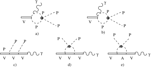
Figure 1: Diagrams considered. The thick dot in the meson-meson vertices indicates final state interaction. V denotes a vector meson, A an axial meson and P a pseudoscalar meson. The intermediate states in the loops can be $K^{+}K^{-}$ or $\pi^{+}\pi^{-}$.

As we can see, the chiral loop contribution is only relevant in the $\rho\rightarrow\pi^{0}\pi^{0}\gamma$ decay.

In the case of the $\phi$ decays[4] the sequential vector exchange diagrams give a small contribution since they occur through an OZI-violating $\phi-\omega$ mixing transition. On the other hand, the chiral loops are the dominant contribution now since the $f_{0}$, $a_{0}$ dominate the amplitudes.

The fact that we have experimental results not only on the integrated branching ratios but also on the invariant mass distributions makes these decays very appealing. In fact, when we compare the theoretical calculation provided by the contributions of diagrams 1a), 1b) and 1c) with the experimental results we see that we get a too narrow distribution in the region of the $f_{0}$, $a_{0}$. The chiral loop contribution is the responsible for the peaks, giving a pole in the right place but not with a sufficiently large width. Therefore, we should take into account more diagrams that have a sizeable effect but have not been considered in the literature when dealing with this problem. These are the unitarized sequential exchange with both an intermediate vector (see 1d)) or axial (see 1e)) particle. The evaluation of diagrams 1d) has been done by using the unitarized amplitudes for the pseudoscalar-pseudoscalar interaction [1]. As for the diagrams with axial resonances, we have built the lowest order Lagrangian consistent with chiral symmetry that accounts for these resonances[5]. This Lagangian is given in eq. 3

$${\cal L}_{BVP} = \tilde{D}<B_{\mu\nu}\{V^{\mu\nu},P\}>$$ (3)

$${\cal L}_{AVP} = i\tilde{F}<A_{\mu\nu}[V^{\mu\nu},P]>$$

where $\tilde{D}$ and $\tilde{F}$ are free parameters, $A$ and $B$ are matrices containing the axial fields, and $P$ and $V$ account for the pseudoscalar and vector mesons, respectively. To fix the values of the free parameters in the Lagrangians we have fitted them to ten different decay channels of axials to a vector and a pseudoscalar. With this we have all the parameters fixed, since the other parameters of the Lagrangians considered are well known and for the integrals we use the same cut-off of 1 GeV as the one used in reference [1] to describe the meson-meson interaction. The final results for the $\phi\rightarrow\pi^{0}\pi^{0}\gamma$ and $\phi\rightarrow\pi^{0}\eta\gamma$ are shown in figures 2 and 3.

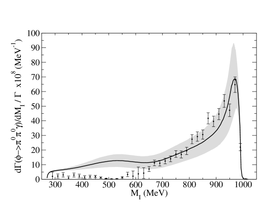
Figure 2: Final results for the $\pi^{0}\pi^{0}$ invariant mass distribution for the $\phi\to\pi^{0}\pi^{0}\gamma$ decay with the theoretical error band. Experimental data from Frascati.

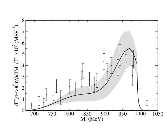
Figure 3: Final results for the $\pi^{0}\eta$ invariant mass distribution for the $\phi\to\pi^{0}\eta\gamma$ decay with the theoretical error band.

3 Conclusions

As we have seen in the previous section, the chiral loops and the sequential vector meson exchange mechanisms provide a good description of the $\rho$ and $\omega$ radiative decays. But in the case of the $\phi$ these two mechanisms are certainly not enough, since the peaks obtained for the scalar resonances are not wide enough. The novelty of this work is the parameter-free inclusion of the unitarized sequential vector exchange and the unitarized sequential axial vector exchange, which helps to widen the distributions in the resonance region. The results obtained are in agreement with the experimental data. The apparent disagreement in the region of around 500 MeV will be most likely solved once the experimental data had been reanalized.

References

- [1] J. A. Oller and E. Oset, Nucl. Phys. A 620, 438 (1997) [Erratum-ibid. A 652, 407 (1997)]
- [2] A. Bramon, R. Escribano, J. L. Lucio Martinez and M. Napsuciale, Phys. Lett. B 517, 345 (2001)
- [3] J. E. Palomar, S. Hirenzaki and E. Oset, Nucl. Phys. A 707, 161 (2002)
- [4] J. E. Palomar, L. Roca, E. Oset and M. J. Vicente Vacas, Nucl. Phys. A 729, 743 (2003)
- [5] L. Roca, J. E. Palomar and E. Oset, arXiv:hep-ph/0306188.