$B$-decays in the heavy-quark expansion

Abstract

Progress in the theoretical description of $B$-meson decays, in particular decays to light hadrons, is reviewed. The factorization properties of such decays can be analyzed using the soft-collinear effective theory. Applications of the effective theory to both inclusive and exclusive decays are discussed.

FERMILAB-CONF-04-309-T
hep-ph/0411065

1 Introduction

The first flavor physics conference I attended was devoted to studying the possibility of a future, second generation, high-luminosity $B$-factory. The title of the conference held in the year 2000 was “Beyond $10^{34}$ $e^{+}e^{-}$ workshop”. Four years later the current $B$-factories at SLAC and KEK have reached luminosities of $10^{34}cm^{-2}s^{-1}$ (the record luminosity, $1.4\times 10^{34}cm^{-2}s^{-1}$, is held by the KEKB accelerator). The impressive performance of the experiments has made it possible to apply methods that were thought to be reserved for future machines, e.g. it is now possible to obtain constraints on the CKM angle $\alpha$ from decays $B\rightarrow\pi\pi$ and $B\rightarrow\rho\rho$ using only the approximate isospin symmetry of the strong interaction as an input. Methods which use data to eliminate all strong interaction physics, like the isospin analysis of the $B\rightarrow\pi\pi$ decays Gronau:1990ka , have the advantage of being conceptually simple and therefore well controlled. The disadvantage of such techniques is that they are experimentally extremely demanding and for this reason the bounds obtained are not (yet) very stringent. More importantly, such methods can only be used to establish new physics but not to explore it, since they rely on the specific structure of the weak interaction in the Standard Model (SM).

In this talk I focus on methods which are more ambitious in that they evaluate part of the strong interaction effects in $B$-decays. All of these tools rely on an expansion of the decay amplitudes in inverse powers of the $b$-quark mass. The predictions obtained are then accurate up to terms suppressed by powers of the heavy-quark mass. The classic example is heavy-quark effective theory (HQET), which has allowed a determination of $|V_{cb}|$ at the level of a few per cent from exclusive semi-leptonic decays. However, HQET is not applicable in $B$-decays in which some of the outgoing, light particles have momenta of the order of the $b$-quark mass, since momenta of this magnitude have been integrated out in the construction of the effective theory. Because of this restriction HQET can in general not be used to analyze $B$-decays involving light hadrons, such as $B\rightarrow\pi\pi$, $B\rightarrow K^{*}\gamma$ or $B\rightarrow\pi\ell\nu$. However, since they probe small CKM elements and flavor changing neutral currents such decays are of great interest to test the Standard Model.

While HQET is not applicable, it is still true that these processes simplify in the heavy-quark limit: the larger the heavy-quark mass, the larger the energies of the outgoing light mesons become and the methods that are used to establish QCD factorization theorems at large momentum transfer become applicable. In this case the hard scale is set by the mass of the heavy $b$-quark, and factorization theorems for inclusive Neubert:1993ch ; Bigi:1993ex ; Korchemsky:1994jb as well as exclusive Beneke:1999br $B$-decays to light hadrons arise in the heavy-quark limit. In the past few years, an effective field theory framework for the analysis of such decays has been developed Bauer:2000yr ; Bauer:2001yt ; Chay:2002vy ; Beneke:2002ph ; Hill:2002vw ; Becher:2003qh : the soft-collinear effective theory (SCET) gives the heavy-quark expansion of heavy-to-light decays and permits the study of their factorization and renormalization properties.

SCET turns out to be more involved than HQET. One complication is that the low energy theory involves multiple scales. In order to get a simple counting of powers of the expansion parameter in such a situation, a single QCD quark (or gluon) field is represented by several effective theory fields whose momentum components scale differently with the heavy-quark mass $m_{b}$. The different effective theory fields are also called modes and correspond to momentum regions, where the QCD diagrams for a given process develop singularities in the heavy-quark limit. In addition to the soft fields present in HQET, SCET contains collinear fields which have large energy and carry large momentum in the direction of the outgoing light hadrons. Another complication is that the non-perturbative input needed in applications of SCET is functional. This is quite generally the case for factorization in hard processes; the most familiar example of such functional input are the parton distribution functions that are needed for the calculation of hadron-hadron scattering processes. The non-perturbative functions relevant in the case of $B$-decays are the light-cone distribution amplitudes of the $B$-meson and the light mesons for exclusive decays and the shape function for inclusive decays.

In my talk I first briefly review HQET and present it in the same diagrammatic language that is used in the construction of SCET. I then discuss the effective theory for inclusive decays to light hadrons, called SCET_I, and sketch how the factorization theorem for these decays is obtained. The effective theory for exclusive decays, SCET_II, is based on the same basic formalism, but contains different degrees of freedom. In applications, one often performs two matching steps. First one matches QCD onto SCET_I at a scale of the order of the $b$-quark mass. At a lower scale $\mu^{2}\sim m_{b}\Lambda$ between the heavy-quark mass and a typical hadronic scale $\Lambda$, one matches SCET_I onto SCET_II. As an example of an exclusive decay which has been analyzed using this two-step procedure, I discuss the factorization properties of the heavy-to-light form factors.

2 The heavy-quark expansion

Weak decays involve a large number of very disparate scales: from very large scales like the mass of the $Z$- and $W$-bosons, and the top quark mass down to very small ones such as the light-quark or the neutrino masses. There are strong interaction effects associated with all of these scales and the effects associated with large scales can be calculated in perturbation theory. To separate the calculable high-energy QCD effects from the non-perturbative low energy physics, one performs expansions in small ratios of the scales in the problem. These expansions are most easily performed by using effective theories which are obtained by integrating out the physics associated with the large scales.

The first step is to expand the weak interactions in $\Lambda/M_{W}\sim\Lambda/M_{Z}\sim\Lambda/m_{t}$, where $\Lambda$ is a momentum component or the mass of one of the lighter particles participating in the weak decay. As a result of this expansion, one obtains the low-energy effective weak Hamiltonian which has the form

$${\cal H}=\frac{G_{F}}{\sqrt{2}}\sum_{i}V^{i}_{\rm CKM}C_{i}(\mu)Q_{i}\,.$$ (1)

The operators $Q_{i}$ are local operators built from the light fields only: since the energies involved in weak decays of hadrons are much smaller than the $W$-, $Z$- and top-mass, these particles are always highly virtual and do not appear as dynamical degrees of freedom at low energies. The operators $Q_{i}$ are multiplied by the CKM factors $V^{i}_{\rm CKM}$ and Wilson coefficients $C_{i}(\mu)$. The Wilson coefficients encode the QCD effects from higher energies. They have been calculated accurately at next-to-leading order in renormalization group improved perturbation theory Buchalla:1995vs . The effective weak Hamiltonians can be viewed as a generalization of the Fermi theory to include all quarks and leptons and their electroweak and strong interactions. The rich phenomenology of hadronic and radiative weak decays (as well as some of the difficulties in their theoretical analysis) result from the fact that the effective Hamiltonian for such decays consists of many operators and a single process can thus involve several different weak decay mechanisms.

For kaon decays the remaining low-energy physics is non-perturbative and one cannot proceed further within perturbation theory. The situation is different for decays of $B$-mesons: the strong coupling constant at the mass of the $b$-quark is $\alpha_{s}(m_{b})\approx 0.2$ so that part of the decay is calculable in perturbation theory. To separate the calculable part one performs an expansion in $1/m_{b}$, the heavy-quark expansion.

2.1 Heavy-to-heavy decays: HQET and the determination of $|V_{cb}|$

The heavy-quark expansion for $B$- to $D$-meson decays was constructed quite some time ago Neubert:1993mb . In the meantime these methods have led to determinations of $|V_{cb}|$ at an accuracy of a few per-cent, from inclusive as well as exclusive measurements. The exclusive determination from the semi-leptonic decay $B^{0}\rightarrow D^{*}\,\ell\nu$ gives HFAG

$$|V_{cb}|=(41.5\pm 1.0_{\rm exp}\pm 1.8_{\rm theo})\times 10^{-3}\,.$$ (2)

To reach an accuracy of 4% in the calculation of an exclusive hadronic decay is quite an achievement. There are several reasons for this success. First of all, it turns out that in the heavy-quark limit, the relevant $B\to D^{*}$ form factor is equal to unity at zero recoil. This prediction receives radiative corrections, suppressed by $\alpha_{s}(m_{Q})$ and non-perturbative power corrections suppressed by $\Lambda/m_{Q}$, where $\Lambda$ is a typical hadronic scale and $m_{Q}$, with $Q=c,b$, is the heavy-quark mass. Both of these corrections are known. The perturbative corrections were calculated to two loops Czarnecki:1997cf . By virtue of Luke’s theorem Luke:1990eg , the first order non-perturbative corrections vanish and the terms of order $\Lambda^{2}/m_{Q}^{2}$ were evaluated with a quenched lattice simulation Hashimoto:2001nb . Preliminary unquenched results are now also available Okamoto:2004xg .

The accuracy is even higher for the inclusive $b\to c$ decay. A recent global fit to all available data yields Bauer:2004ve

$$|V_{cb}|=(41.9\pm 0.6)\times 10^{-3}\,.$$ (3)

The explanation for the tiny uncertainty is similar to the exclusive case: in the heavy-quark limit the decay rate is given by the $b$-quark decay rate and the leading corrections of order $\alpha_{s}$ or $\Lambda^{2}/m_{b}^{2}$ to this predictions have also been evaluated. The non-perturbative corrections to the decay rate are given by the $B$-meson matrix elements of the two operators that appear in the sub-leading HQET Lagrangian. One of these matrix elements can be related to the the experimental value of the mass difference between pseudoscalar and vector $B$-mesons. The second one as well as the $b$- and $c$-quark masses can be obtained from the experimental results for moments of the decay spectrum, which depend on the same parameters as the total rate. The analysis of these moments has been done independently by two groups Bauer:2002sh ; Gambino:2004qm who at this point accuse each other in turn of underestimating their theoretical uncertainties and algebraic mistakes Bauer:2004ve ; Uraltsev:2004ra .

Before discussing the heavy-to-light hadron decays, I would like to show how the HQET Lagrangian can be derived by expanding QCD Feynman diagrams around the heavy-quark limit. The same diagrammatic techniques are used in the construction of the SCET Lagrangian, discussed in the next section. At tree level the expansion is achieved after realizing that at low energies, the heavy quark is close to its mass shell so that the heavy-quark momentum can be written as $p_{Q}=m_{Q}v_{\mu}+r_{\mu}$, where $v^{2}=1$ and all components of the residual momentum $r_{\mu}$ are small compared to $m_{Q}$. The expansion of the heavy-quark propagator then reads

$$\frac{p_{Q}\!\!\!\!\!\!\!\!\!/\,\,\,+r\!\!\!\!/+m_{Q}}{(p_{Q}+r)^{2}-m_{Q}^{2}}=\frac{1+v\!\!\!\!/}{2}\frac{1}{v\cdot r}+\dots\,.$$ (4)

Note that ${\rm P}_{+}=\frac{1+v\!\!\!\!/}{2}$ is a projector, ${\rm P}_{+}^{2}={\rm P}_{+}$. Since it appears sandwiched between heavy-quark propagators, the quark-gluon vertex also simplifies and becomes

$${\rm P}_{+}\,ig\,A\!\!\!\!\!/\,{\rm P}_{+}=ig\,v\cdot A\,{\rm P}_{+}\,.$$ (5)

It is easy to write a Lagrangian that yields the above propagator and vertex, namely

$${\cal L}_{\rm HQET}=\bar{h}\,{\rm P}_{+}\,i\,v\cdot D\,h\,.$$ (6)

The field $h$ is the heavy-quark field in HQET. Since the Lagrangian involves the projector ${\rm P}_{+}$, the field $h$ is is effectively only a two component field.

For loop graphs, simply expanding the heavy-quark propagators in the integrand does not give the correct result for the expansion of the integral. The problem is that the loop momentum flowing through the heavy-quark propagator is large in some momentum regions, so that the expansion (4) is not always appropriate. However, in dimensional regularization the prescription to obtain the correct result is remarkably simple. What one needs to do is to perform two different expansions: first, one assumes the loop momentum to be small, of order $r_{\mu}$, expands the integrand and then performs the loop integration without any restriction on the integration. The contribution obtained in this way is called the soft part of the integral. In general, the soft part has ultraviolet divergences not present in the original integral. These extra divergences are regulated by dimensional regularization and manifest themselves as poles in $d-4$. One then expands the loop integrand a second time, this time assuming all components of the loop momentum to be large, of the order of the $b$-quark mass. This second part is called the hard part of the integral and it has infrared divergences that are again regulated dimensionally. In the sum the infrared divergences of the hard part cancel against the ultraviolet divergences of the soft part and expansion of full integral is recovered after adding the hard and the soft part. This technique for performing asymptotic expansions of integrals is also called the strategy of regions Smirnov:2002pj .

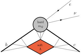
Figure 1: Semi-leptonic $B\to D$ decay. The thick lines denote the heavy quarks. The dotted lines represent soft light quarks and gluons.

While the contribution of the soft region corresponds to the effective theory Feynman diagrams, the hard part is absorbed into the Wilson coefficients of the effective theory operators. For the Lagrangian (6) of a single heavy quark at leading order, the only effect of the hard contributions is to change the normalization of the field $h$. Since the normalization is not a physical observable, it is not really necessary to introduce a Wilson coefficient to reproduce this effect.

To analyze the exclusive semileptonic $B\rightarrow D$ decay, one introduces two copies of the heavy-quark Lagrangian (6), one for the $b$-quark and another one for the $c$-quark. The four-velocity vector $v$ needed to remove the large part of the heavy-quark momenta will be different for the two quarks. However, also in this case only two momentum regions, hard and soft, are relevant, as illustrated in Figure 1. The hard-corrections are given by the Wilson coefficient of the heavy-to-heavy current operator and depend on the scalar product of the two heavy-quark velocities Falk:1990cz ; Neubert:1991tg .

2.2 Inclusive heavy-to-light decays: SCET_I

In order to obtain the decay rate of the inclusive semi-leptonic decay, one uses the optical theorem and calculates the imaginary part of the forward matrix element of two weak currents

$$T^{\mu\nu}=i\,\int d^{4}x\,e^{iqx}\,\langle\bar{B}(p_{B})|\mbox{\bf T}\left\{J^{\dagger\mu}(0),J^{\nu}(x)\right\}|\bar{B}(p_{B})\rangle\,,$$ (7)

where $J^{\mu}=\bar{u}\gamma^{\mu}\,(1-\gamma_{5})b$. To calculate the total rate, one then uses the Operator Product Expansion (OPE) which corresponds to the expansion of the total rate around the heavy-quark limit Chay:1990da . At leading order in the expansion one finds that the total rate of the meson decay is equal to the free heavy quark decay rate up to calculable radiative corrections.

Unfortunately, it is experimentally necessary to impose rather severe kinematic cuts to discriminate the $B\rightarrow X_{u}\ell\nu$ and $B\rightarrow X_{s}\gamma$ decays against the background. Such cuts typically enforce a small invariant mass of the system of outgoing hadrons $M_{X}^{2}\sim\Lambda\,m_{b}\ll E_{X}^{2}\sim m_{b}^{2}$ and lead to a breakdown of the OPE. In the heavy-quark limit, the enhanced higher order terms can be resummed into a non-perturbative shape function $S$ and for this reason the region of small $M_{X}$ is also called the shape-function region Neubert:1993ch ; Bigi:1993ex . The same function appears in the semi-leptonic and the radiative decays and one obtains a relation between the decay rates. To perform the perturbative analysis of the factorization properties of the partial decay rate in the shape function region, one replaces the in- and outgoing mesons with interpolating currents and studies the vacuum expectation value of the correlator of the weak current with the two meson currents. The structure of the diagrams contributing to this correlator is shown in Figure 2.

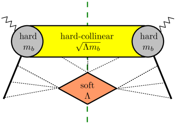
Figure 2: Inclusive semi-leptonic $B$-decay. The differential decay rate is obtained from the imaginary part of the forward matrix element of two weak currents. The thick line denotes the heavy $b$-quark. The dotted lines represent soft quarks and gluons.

It turns out that the hard and soft momentum regions are not sufficient to obtain the heavy-quark expansion of the diagrams relevant for the heavy-to-light decays. The reason is that the decay of the heavy quark typically produces a jet of energetic light particles. Since their energies are of the order of the $b$-quark mass they cannot be described by the soft fields present in HQET and require the introduction of additional, so-called collinear fields. In HQET one uses the reference unit vector $v_{\mu}$ to isolate the large part of the $b$-quark four-momentum, a common choice is $v_{\mu}=(1,0,0,0)$; in SCET, one introduces in addition a light-like reference vector, $n_{\mu}=(1,0,0,1)$, in the direction of the jet of energetic, outgoing, light particles and decomposes all momenta as

$$p_{\mu}=n\cdot p\,\frac{\bar{n}_{\mu}}{2}+\bar{n}\cdot p\,\frac{n_{\mu}}{2}+p_{\mu}^{\perp}\,=p_{+}^{\mu}+p_{-}^{\mu}+p_{\perp}^{\mu},$$ (8)

where ${\bar{n}}_{\mu}=2v_{\mu}-n_{\mu}=(1,0,0,-1)$. The leading order of the heavy-quark expansion of the diagrams in Figure 2 was first analyzed in Korchemsky:1994jb , where it was shown that three momentum regions lead to singularities in these diagrams. The scaling of the momentum components $(n\cdot p,\bar{n}\cdot p,p_{\mu}^{\perp})$ in these regions is

hard: $$(m_{b}, m_{b}, m_{b}),$$ (9)

hard-collinear: $$(\Lambda, m_{b}, \sqrt{\Lambda\,m_{b}}),$$

soft: $$(\Lambda, \Lambda, \Lambda).$$

Interestingly, an intermediate scale $\mu_{hc}=\sqrt{\Lambda\,m_{b}}$ appears, whose virtuality lies between the small virtuality $\Lambda\sim M_{B}-m_{b}$ of the external lines and the mass of the heavy quark. The presence of three scales also manifests itself in the factorization formula for the inclusive decay rate Korchemsky:1994jb

$$d\Gamma\sim H\,J\otimes S\,.$$ (10)

The function $H$ contains the hard corrections, the jet-function $J$ the contribution from the hard-collinear region and the shape function $S$ the soft contribution. The symbol “$\otimes$” indicates the convolution of the jet-function with the shape function. Let me note that while it is simple to see that the above three momentum regions are necessary to obtain the expansion of the diagrams in Figure 2, so far no formal proof has been given that these three regions are sufficient to obtain the expansion of an arbitrary multi-loop diagram.

To construct the effective theory, one introduces the soft quark field $q$, the soft gluon field $A_{s}^{\mu}$, the heavy-quark field $h$ and the hard-collinear quark and gluon fields $\xi$ and $A_{hc}^{\mu}$. The momentum components of these fields scale as in (9) and the scaling of the field components can be inferred by inspecting the propagators of the fields. One constructs the Lagrangian for these fields in such a way that its Feynman rules give the QCD diagrams expanded in the soft and collinear momentum regions. The technical details of the construction of the effective Lagrangian are beyond the scope of this talk, but let me illustrate some of its features using the leading order Lagrangian

$${\cal L}_{\rm SCET}^{(0)}=\bar{\xi}\frac{\bar{n}\!\!\!/}{2}\left(in\cdot D_{hc}+g\,n\cdot A_{s}(x_{-})+i{D\!\!\!\!\!/}_{\perp hc}\frac{1}{i\bar{n}\cdot D_{hc}}\,i{D\!\!\!\!\!/}_{\perp hc}\right)\xi\\ +\bar{q}\,iD_{s}\!\!\!\!\!\!\!\!/\,\,\,\,q+\bar{h}iv\cdot D_{s}h+{\cal L}^{(0)}_{\rm YM}.$$ (11)

The purely soft terms on the second line are exactly the leading order HQET Lagrangian. The hard-collinear quark Lagrangian has a more complicated form because not all four components of a hard-collinear quark field scale with the same power of $\Lambda/m_{b}$. One can split the original Dirac field into two-component fields $\xi$ and $\eta$

$$\psi_{hc}=\left(\frac{n\!\!\!\!/\,\bar{n}\!\!\!\!/}{4}+\frac{\bar{n}\!\!\!\!/\,n\!\!\!\!/}{4}\right)\psi_{hc}=\xi+\eta$$ (12)

so that $n\!\!\!\!/\xi=\bar{n}\!\!\!\!/\eta=0$. The field $\eta$ is suppressed by a power of $(\Lambda/m_{b})^{1/2}$ with respect to $\xi$ and can be integrated out. Since no approximation is made when $\eta$ is integrated out, the hard-collinear part of the Lagrangian (11) is, despite appearances, equivalent to the usual QCD quark Lagrangian. Finally, let me discuss the interaction term $g\,\bar{\xi}(x)\frac{\bar{n}\!\!\!\!\!/}{2}\,{n\cdot A_{s}(x_{-})}\xi(x)$. The interaction is simpler than the usual QCD quark-gluon coupling for two reasons. First of all, it only involves a single component of the soft gluon field. This is a consequence of the projection properties of the hard-collinear quark spinor $\bar{\xi}\gamma_{\perp}^{\mu}\xi=\bar{\xi}n\!\!\!\!/\,\xi=0$. Secondly, the soft gluon field only depends on the single coordinate $x_{-}=\bar{n}\cdot x\frac{n_{\mu}}{2}$. To obtain diagrams expanded in momentum space, one has to perform a derivative expansion of the effective Lagrangian in position space Beneke:2002ph : in interactions with collinear fields the soft fields are expanded as

$$\phi_{s}(x)=\phi_{s}(x_{-})+x_{\perp}\cdot\partial\phi_{s}(x_{-})+x_{+}\cdot\partial\phi_{s}(x_{-})+\dots\,.$$ (13)

Alternatively, one can use a hybrid position and momentum space representation of the collinear fields, the label formalism Bauer:2000yr . Because of the expansion (13), the interaction terms in the Lagrangian (11) are not translation invariant. However, the invariance is restored order by order after including higher order terms. Let me briefly comment on the gauge transformation properties of the above fields. One can perform separate gauge transformations on the two gluon fields $A_{s}$ and $A_{hc}$. The form of these transformations is restricted by the requirement that they should respect the power counting of the fields and the fact that the sum of the two gluon fields $A_{s}+A_{hc}$ has to transform as the usual QCD gluon field. The explicit form of the gauge transformations as well as the first three orders of the SCET Lagrangian can be found in Beneke:2002ni . In the label formalism, the sub-leading Lagrangian was given in Pirjol:2002km .

In order to analyze the inclusive semi-leptonic decay one needs the weak current $J_{\mu}$ in the effective theory. At leading order this current is represented in the effective theory as

$$J^{\mu}(x)=\sum_{i=1}^{3}\int\!ds\,\,C_{i}(s)\,e^{-im_{b}v\cdot x}\,J^{\mu}_{i}(x,s)\,.$$ (14)

The three leading order effective theory current operators are

$$J^{\mu}_{i}(x,s)=\bar{\xi}(x+s\bar{n})W_{hc}\,(1+\gamma_{5})\,\Gamma^{\mu}_{i}\,h(x_{-})\,\text{ with }\Gamma^{\mu}_{1,2,3}=\{\gamma^{\mu},v^{\mu},n^{\mu}\}\,.$$ (15)

The SCET current operators are nonlocal along the light ray in the $\bar{n}$-direction. This is a consequence of the fact that the $\bar{n}\cdot\partial$-derivative on a hard-collinear field counts as a quantity of order one and arbitrary powers of this derivative can appear at any given order in the expansion in $\Lambda/m_{b}$. The light-like, hard-collinear Wilson line $W_{hc}$ ensures gauge invariance of the operator and the phase factor $e^{-im_{b}v\cdot x}$ relates the heavy quark field $h$ to the QCD $b$-quark field.

To obtain the SCET representation of the current correlator $T^{\mu\nu}$ one inserts the above representation (14) of the current into (7). Since the initial and final state $B$-meson in (7) do not contain collinear partons, one can perform a second matching step and integrate out the hard-collinear fields in the products of effective theory currents:

$$J_{i}^{\dagger\mu}(0,t)J_{j}^{\nu}(x,s)=\bar{h}(0)\,\Gamma_{i}^{\mu}\,W^{\dagger}_{hc}\,\xi(t\bar{n})\,\bar{\xi}(x+s\bar{n})W_{hc}\,\Gamma^{\nu}_{j}\,h(x_{-})\\ \rightarrow{\cal J}(x+(s-t){\bar{n}})\,\bar{h}(0)\,\Gamma_{i}^{\mu}\,\frac{\bar{n}\!\!\!\!/}{2}\,\Gamma_{j}^{\nu}\,h(x_{-})+\dots\,.$$ (16)

The Wilson coefficient ${\cal J}$ that appears in this second step is called the jet-function. After realizing that the matrix elements of the operators $\bar{h}(0)\,\Gamma_{i}^{\mu}\frac{\bar{n}\!\!\!\!/}{2}\Gamma_{j}^{\nu}\,h(x_{-})$ can be related to the matrix element of the single operator $\bar{h}(0)\,h(x_{-})$ by heavy-quark symmetry and rewriting these above results in momentum space, one obtains the factorization theorem (10).

While the factorization theorem was originally derived diagrammatically, the SCET analysis has led to several improvements in our understanding of these decays. First of all, solving the renormalization group equations in the effective theory at the next-to-leading order, the perturbative single and double logarithms of the different scale ratios in the hard and the jet-functions have been resummed at next-to-leading order and predictions for the various decay spectra have been obtained Bauer:2003pi ; Bosch:2004th , which are free of the spurious Landau pole singularities present in earlier work Korchemsky:1994jb ; Akhoury:1995fp ; Leibovich:1999xf . Also, because of the renormalization properties of the shape function, the relation between its moments and higher order HQET parameters is more complicated than previously assumed Bauer:2003pi ; Bosch:2004th .

The SCET formalism has also been used to investigate the partial $B\rightarrow X_{s}\gamma$ decay rate with a cut $E_{\gamma}>E_{0}$ on the photon energy . For low values of this cut, the rate can be calculated using the standard OPE, while for larger values higher order effects become large and have to be resummed into the shape function. The transition between the two regimes is smooth: in the presence of a photon energy cut, the OPE becomes an expansion in $1/\Delta$, where $\Delta=m_{b}-2E_{0}$ is the energy window available after the cut. Another effect of the cut is that the rate calculated in the OPE gets perturbative corrections of order $\alpha_{s}(\Delta)$ . For realistic values of the cut the scale $\Delta$ is not much larger than 1GeV. After an analysis in renormalization group improved perturbation theory, Neubert finds that, even for the low value $E_{0}=1.8\,{\rm GeV}$, higher order perturbative corrections to the cut rate are sizable, of order 15% Neubert:2004dd . This is larger than previously estimated and larger than the power corrections of order 10%.

As the above discussion shows, the effective theory analysis of the inclusive decay rate reduces to the analysis of the weak heavy-to-light current. This analysis has been extended to sub-leading order in $\Lambda/m_{b}$ Bauer:2001mh ; Bauer:2002yu ; Lee:2004ja ; Bosch:2004cb . While a single non-perturbative shape function is sufficient to obtain the leading order rate, several shape functions appear at the next order. At leading order, one can determine $|V_{ub}|$ by taking a ratio of weighted $B\rightarrow X_{u}\ell\nu$ and $B\rightarrow X_{s}\gamma$ decay spectra for which the shape function effects drop out. An understanding of the corrections to this relation from sub-leading shape functions is important for a precise determination of $|V_{ub}|$.

2.3 Exclusive heavy-to-light decays: SCET_II

It turns out that exclusive $B$-decays have a more complicated structure than the inclusive decays studied in the previous section. To analyze the decays diagrammatically, one again replaces the mesons with interpolating currents. For example, in order to analyze the $B\rightarrow\pi$ form factor of a current $J_{\Gamma}^{\mu}(0)$, one uses the relation

$$\int\!d^{4}x\,\int\!d^{4}y\,e^{ip_{\pi}x-ip_{B}y}\langle 0\,|\,T\left\{J^{\dagger}_{B}(x)J_{\Gamma}^{\mu}(0)J_{\pi}(y)\right\}\,|\,0\rangle\\ =\frac{if_{B}^{(J)}}{p_{B}^{2}-M_{B}^{2}}\frac{if_{\pi}^{(J)}}{p_{\pi}^{2}-M_{\pi}^{2}}\,\langle\pi(p_{\pi})|\,J_{\Gamma}(0)\,|B(p_{B})\rangle+\dots$$ (17)

and analyzes the factorization properties of the correlator on the left-hand side diagrammatically.

Here, the currents $J_{B}$ and $J_{\pi}$ have the quantum numbers of the $B$-meson and the pion respectively and associated decay constants $f_{B}^{(J)}$ and $f_{\pi}^{(J)}$. The ellipsis denotes terms that do not have a pole at $p_{B}^{2}=m_{B}^{2}$ with $p_{B}^{0}<0$ and $p_{\pi}^{2}=m_{\pi}^{2}$ with $p_{\pi}^{0}>0$.

$p_{B}\,$ $p_{\pi}$

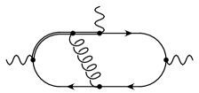
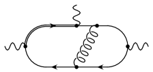
Figure 3: Lowest order QCD diagrams contributing to the correlator (17). The double line denotes the heavy quark.

The lowest order diagrams contributing to the correlator (17) are shown in Figure 3. The following momentum regions are needed to obtain their expansion Becher:2003qh

hard: $$(m_{b}, m_{b}, m_{b}),$$ (18)

hard-collinear: $$(\Lambda, m_{b}, \sqrt{\Lambda\,m_{b}}),$$

collinear: $$(\Lambda^{2}/m_{b}, m_{b}, \Lambda),$$

soft: $$(\Lambda, \Lambda, \Lambda),$$

soft-collinear: $$(\Lambda^{2}/m_{b}, \Lambda, \sqrt{\Lambda^{3}/m_{b}}),$$

where the three components denote the scaling of $(n\cdot p,\bar{n}\cdot p,p_{\perp})$ and $\Lambda$ stands for a hadronic scale in the problem that is independent of $m_{b}$. The occurrence of a collinear region in addition to the hard-collinear region is easily understood: the scaling of its components is the same as that of the external pion momentum. Since $p_{\pi}^{2}$ is independent of the $b$-quark mass, the hard-collinear scaling would not be appropriate. What is surprising is the presence of an additional region with very low virtuality: the soft-collinear region with $p^{2}_{sc}=\Lambda^{3}/m_{b}$. In the effective theory, these soft-collinear fields represent a low energy interaction between the collinear and soft sectors. The scaling of their momentum components is such that they can be emitted and absorbed by both soft and collinear particles without taking either of them off-shell. An example of a diagram where a soft-collinear contribution appears is the first diagram in Figure 3, which gets a contribution when the spectator quark is soft-collinear and almost all external momentum flows through the current quarks.

If these soft-collinear fields contribute to a given quantity in perturbation theory, factorization is explicitly violated. Since they are the only low energy interaction between the collinear and soft sectors, the opposite is also true: if they do not contribute to a given quantity, the quantity factorizes. Clearly, the physics associated with the soft-collinear fields cannot be calculated reliably in perturbation theory: as soon as there is such a contribution, the corresponding quantity will be deemed non-perturbative. The assumption on which the factorization framework relies is that if one does not find a violation of factorization in perturbation theory the quantity indeed factorizes.

Unfortunately, even the seemingly simplest decays, namely the heavy-to-light meson form-factors, do not factorize in the heavy-quark limit. At large recoil energies $E\sim M_{B}/2$, they take the form Beneke:2000wa

$$F_{i}^{B\to M}(E)=C_{i}(E)\,\zeta_{M}(E)+\int_{0}^{\infty}\!{d\omega\over\omega}\,\phi_{B}(\omega)\int_{0}^{1}\!du\,f_{M}\,\phi_{M}(u)\,T_{i}(E,\omega,u)\,,$$ (19)

up to corrections suppressed by $1/m_{b}$. The non-factorizable piece is given by the non-perturbative function $\zeta_{M}(E)$ that depends on the momentum transfer. The remainder factorizes into a convolution of a hard scattering kernel $T_{i}(E,\omega,u)$ with the light-cone distribution amplitudes $\phi_{B}(\omega)$ and $\phi_{M}(u)$ of the two mesons. The coefficients $C_{i}(E)$ and the kernels $T_{i}(E,\omega,u)$ are Wilson coefficients of effective theory operators. While the form factors do not factorize, one obtains relations between different form factors because the function $\zeta_{M}(E)$ is independent of the Dirac structure of the current under consideration Charles:1998dr . In this respect the situation is rather similar to the case of the $B\rightarrow D$ transition form factors, which in the heavy-quark limit can be expressed in terms of a single function, the Isgur-Wise function, up to perturbative corrections Isgur:1989ed .

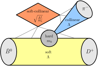
Figure 4: Momentum regions in the perturbative analysis of the exclusive decay $B\rightarrow D\pi$.

The heavy-to-light form factors are in a sense sub-leading quantities, since the superficially leading term in a diagrammatic analysis happens to vanish. By naive power counting, one would expect the third diagram in Figure 3 to be the leading contribution, but upon closer inspection one finds that the expansion of all three diagrams starts at the same order. In the effective theory this manifests itself in the fact that one needs to include sub-leading current operators to analyze the form factor to leading order. To perform the analysis, one first matches QCD onto SCET_I. The leading order effective theory currents have been discussed in the previous section, see (15). The reason for the above mentioned symmetry relations between the different form factors is that both the heavy and the hard-collinear light quark field are represented by two component fields. Two types of current operators appear at next-to-leading order: operators with an additional derivative $\partial^{\mu}_{\perp}$ on the hard-collinear quark and operators with an additional hard-collinear gluon field $A_{hc\perp}^{\mu}$. The operators with an additional derivative have the same Wilson coefficients as the leading operators and their matrix elements fulfill the same symmetry relations. The matrix elements of the remaining sub-leading operators which contain an additional hard-collinear gluon field $A_{hc\perp}^{\mu}$ violate the symmetry relations. To prove the factorization theorem (19), one matches them onto SCET_II and shows that their contribution to the form factors factorizes. This analysis has been carried out and the formula (19) was established recently Bauer:2002aj ; Beneke:2003pa ; Lange:2003pk . Also, the matching calculations have been performed to one-loop order. The coefficients $C_{i}$ were determined in Bauer:2000yr ; Beneke:2004rc , and the two matching steps for $T_{i}$ were performed in Hill:2004if ; Beneke:2004rc ; Becher:2004kk . The hard scattering kernels contain single and double (or Sudakov) logarithms of large scale ratios. These logarithms can be resummed by solving the renormalization group equations in the effective theory, which was done in Hill:2004if . The analysis in this paper also allows one to categorize the relations between the different form factors: generically, one can expect corrections of the order of $\alpha_{s}$ at the hard-collinear scale $\mu_{hc}^{2}\sim\Lambda\,m_{b}$. In some cases, however, the corrections only involve $\alpha_{s}$ at the hard scale and some relations do not receive radiative corrections at all richardQCD04 . The heavy-to-light form factors are an important element of the factorization theorem for the phenomenologically important decays to two light mesons $B\rightarrow M_{1}\,M_{2}$. Using the factorization theorem for these decays Beneke:1999br , predictions for the complete set of the almost one hundred $B^{-}$, $B^{0}$ and $B_{s}$ decay modes are given in Beneke:2003zv . These decays have been investigated using SCET Chay:2003zp ; Bauer:2004tj , but a complete analysis is not yet available.

The decays $B\rightarrow DM$, depicted in Figure 4, have a simpler structure. In this case an analysis using the effective theory at leading order is sufficient and the soft-collinear mode does not contribute in the heavy-quark limit. The amplitude factorizes into a soft part (the $B\rightarrow D$ form-factor at zero momentum transfer) and a collinear part which is given by the pion light-cone distribution amplitude and is convoluted with a hard scattering kernel Dugan:1990de ; Politzer:1991au ; Beneke:2000ry ; Bauer:2001cu . Using the effective theory framework, also the power suppressed neutral decay modes $B^{0}\rightarrow D^{(*)0}M^{0}$ have been analyzed recently and it was found that the branching ratios as well as the strong phases are equal for the decay to the vector and pseudoscalar $D$-meson Mantry:2003uz ; Mantry:2004pg ; blechman . Analogous relations also hold for non-leptonic $b\rightarrow c$ decays of baryons Leibovich:2003tw .

3 Summary

The techniques used to analyze hard-scattering factorization at large momentum transfer can also be used to analyze decays of heavy to light hadrons in the heavy-quark limit. While based on the same theoretical concepts, the factorization theorems for exclusive heavy-to-light decays are complicated in that the naively leading order term vanishes and one has to perform the diagrammatic analysis to sub-leading order. SCET allows one to perform this analysis in a controlled and transparent way. The effective theory fields correspond to the momentum regions in which the diagrams develop singularities and the hard scattering part of these processes is encoded in the Wilson coefficients of the effective theory operators. The resummation of large perturbative logarithms is achieved by solving the RG evolution equation of the corresponding operators.

Since the hard scale for these decays is given by the $b$-quark mass, it is numerically smaller than typical momentum transfers in hard processes at colliders. An understanding of the size of the power corrections is therefore important. Using the effective theory framework, these power corrections have been worked out and estimated for the inclusive semi-leptonic decays. For the exclusive decays, we have not yet reached the same level of accuracy because the leading terms in the amplitudes in general already involve the sub-leading Lagrangian. An important achievement was the analysis of the heavy-to-light form factors and the proof of the factorization theorem for this case. Using the same techniques, a complete analysis of the factorization properties of the charmless two-body decays is within reach. Some of the power corrections for these decays have been identified and estimated, but no complete treatment is available to date. While such an analysis seems difficult, it is important: Our capability to explore new flavor physics in $B$-decays can only be as good as our understanding of the strong interaction physics in their decays.

References

- (1) M. Gronau and D. London, Phys. Rev. Lett. 65, 3381 (1990).
- (2) M. Neubert, Phys. Rev. D 49, 3392 (1994) [hep-ph/9311325], Phys. Rev. D 49, 4623 (1994) [hep-ph/9312311].
- (3) I. I. Y. Bigi, M. A. Shifman, N. G. Uraltsev and A. I. Vainshtein, Int. J. Mod. Phys. A 9, 2467 (1994) [hep-ph/9312359].
- (4) G. P. Korchemsky and G. Sterman, Phys. Lett. B 340, 96 (1994) [hep-ph/9407344].
- (5) M. Beneke, G. Buchalla, M. Neubert and C. T. Sachrajda, Phys. Rev. Lett. 83, 1914 (1999) [hep-ph/9905312].
- (6) C. W. Bauer, S. Fleming, D. Pirjol and I. W. Stewart, Phys. Rev. D 63, 114020 (2001) [hep-ph/0011336].
- (7) C. W. Bauer, D. Pirjol and I. W. Stewart, Phys. Rev. D 65, 054022 (2002) [hep-ph/0109045].
- (8) J. Chay and C. Kim, Phys. Rev. D 65, 114016 (2002) [hep-ph/0201197].
- (9) M. Beneke, A. P. Chapovsky, M. Diehl and T. Feldmann, Nucl. Phys. B 643, 431 (2002) [hep-ph/0206152].
- (10) R. J. Hill and M. Neubert, Nucl. Phys. B 657, 229 (2003) [hep-ph/0211018].
- (11) T. Becher, R. J. Hill and M. Neubert, Phys. Rev. D 69, 054017 (2004) [hep-ph/0308122].
- (12) For a review see: G. Buchalla, A. J. Buras and M. E. Lautenbacher, Rev. Mod. Phys. 68, 1125 (1996) [hep-ph/9512380].
- (13) For a review see: M. Neubert, Phys. Rept. 245, 259 (1994) [hep-ph/9306320].
- (14) Heavy Flavor Averaging Group: http://www.slac.stanford.edu/xorg/hfag/.
- (15) A. Czarnecki, Phys. Rev. Lett. 76, 4124 (1996) [hep-ph/9603261]. A. Czarnecki and K. Melnikov, Nucl. Phys. B 505, 65 (1997) [hep-ph/9703277].
- (16) M. E. Luke, Phys. Lett. B 252, 447 (1990).
- (17) S. Hashimoto, A. S. Kronfeld, P. B. Mackenzie, S. M. Ryan and J. N. Simone, Phys. Rev. D 66, 014503 (2002) [hep-ph/0110253].
- (18) M. Okamoto et al., hep-lat/0409116.
- (19) C. W. Bauer, Z. Ligeti, M. Luke, A. V. Manohar and M. Trott, hep-ph/0408002.
- (20) C. W. Bauer, Z. Ligeti, M. Luke and A. V. Manohar, Phys. Rev. D 67, 054012 (2003) [hep-ph/0210027].
- (21) P. Gambino and N. Uraltsev, Eur. Phys. J. C 34, 181 (2004) [hep-ph/0401063].
- (22) N. Uraltsev, hep-ph/0409125.
- (23) For a review see: V. A. Smirnov, “Applied asymptotic expansions in momenta and masses,” (Springer tracts in modern physics. 177), Springer (2002) Berlin, Germany.
- (24) A. F. Falk and B. Grinstein, Phys. Lett. B 249, 314 (1990).
- (25) M. Neubert, Phys. Rev. D 46, 2212 (1992).
- (26) J. Chay, H. Georgi and B. Grinstein, Phys. Lett. B 247, 399 (1990).
- (27) M. Beneke and T. Feldmann, Phys. Lett. B 553, 267 (2003) [hep-ph/0211358].
- (28) D. Pirjol and I. W. Stewart, Phys. Rev. D 67, 094005 (2003) [Erratum-ibid. D 69, 019903 (2004)] [hep-ph/0211251].
- (29) C. W. Bauer and A. V. Manohar, Phys. Rev. D 70, 034024 (2004) [hep-ph/0312109].
- (30) S. W. Bosch, B. O. Lange, M. Neubert and G. Paz, Nucl. Phys. B 699, 335 (2004) [arXiv:hep-ph/0402094].
- (31) R. Akhoury and I. Z. Rothstein, Phys. Rev. D 54, 2349 (1996) [hep-ph/9512303].
- (32) A. K. Leibovich, I. Low and I. Z. Rothstein, Phys. Rev. D 61, 053006 (2000) [hep-ph/9909404].
- (33) M. Neubert, hep-ph/0408179.
- (34) C. W. Bauer, M. E. Luke and T. Mannel, Phys. Rev. D 68, 094001 (2003) [hep-ph/0102089].
- (35) C. W. Bauer, M. Luke and T. Mannel, Phys. Lett. B 543, 261 (2002) [hep-ph/0205150].
- (36) K. S. M. Lee and I. W. Stewart, hep-ph/0409045.
- (37) S. W. Bosch, M. Neubert and G. Paz, hep-ph/0409115.
- (38) M. Beneke and T. Feldmann, Nucl. Phys. B 592, 3 (2001) [hep-ph/0008255].
- (39) J. Charles, A. Le Yaouanc, L. Oliver, O. Pene and J. C. Raynal, Phys. Rev. D 60, 014001 (1999) [hep-ph/9812358].
- (40) N. Isgur and M. B. Wise, Phys. Lett. B 237, 527 (1990).
- (41) C. W. Bauer, D. Pirjol and I. W. Stewart, Phys. Rev. D 67, 071502 (2003) [hep-ph/0211069].
- (42) M. Beneke and T. Feldmann, Nucl. Phys. B 685, 249 (2004) [hep-ph/0311335].
- (43) B. O. Lange and M. Neubert, Nucl. Phys. B 690, 249 (2004) [hep-ph/0311345].
- (44) R. J. Hill, T. Becher, S. J. Lee and M. Neubert, JHEP 0407, 081 (2004) [hep-ph/0404217].
- (45) M. Beneke, Y. Kiyo and D. s. Yang, Nucl. Phys. B 692, 232 (2004) [hep-ph/0402241].
- (46) T. Becher and R. J. Hill, hep-ph/0408344.
- (47) R. J. Hill, “Symmetry relations for heavy-to-light form factors at large recoil,” to appear in the proceedings of the 11th International QCD Conference, Montpellier, July 5-10, 2004.
- (48) M. Beneke and M. Neubert, Nucl. Phys. B 675, 333 (2003) [hep-ph/0308039].
- (49) J. g. Chay and C. Kim, Phys. Rev. D 68, 071502 (2003) [hep-ph/0301055].
- (50) C. W. Bauer, D. Pirjol, I. Z. Rothstein and I. W. Stewart, hep-ph/0401188.
- (51) M. J. Dugan and B. Grinstein, Phys. Lett. B 255, 583 (1991).
- (52) H. D. Politzer and M. B. Wise, Phys. Lett. B 257, 399 (1991).
- (53) M. Beneke, G. Buchalla, M. Neubert and C. T. Sachrajda, Nucl. Phys. B 591, 313 (2000) [hep-ph/0006124].
- (54) C. W. Bauer, D. Pirjol and I. W. Stewart, Phys. Rev. Lett. 87, 201806 (2001) [hep-ph/0107002].
- (55) S. Mantry, D. Pirjol and I. W. Stewart, Phys. Rev. D 68, 114009 (2003) [hep-ph/0306254].
- (56) S. Mantry, hep-ph/0405290.
- (57) A. E. Blechman, S. Mantry, I. W. Stewart, hep-ph/0410312.
- (58) A. K. Leibovich, Z. Ligeti, I. W. Stewart and M. B. Wise, Phys. Lett. B 586, 337 (2004) [hep-ph/0312319].