Abstract

I review recent progress on exclusive $B$ meson decays made in the perturbative QCD approach, concentrating on the evolution of the $B$ meson wave function in $k_{T}$ factorization, radiative decays, polarizations in $VV$ modes, and new physics effect in $B\to\phi K_{S}$.

1 Introduction

Exclusive $B$ meson decays are important for extracting the fundamental Standard Model parameters, such as the Cabibbo-Kobayashi-Maskawa (CKM) matrix elements, and for exploring new physics. They are complicated due to strong dynamics, which must be well understood in order to achieve the above goals. Especially, QCD theories for two-body nonleptonic decays are necessary. Several approaches based on different factorization theorems have been developed, which include perturbatiove QCD (PQCD) [1, 2, 3], QCD-improved factorization (QCDF) [4], soft-collinear effective theory (SCET) [5, 6], light-cone sum rules (LCSR) [7, 8, 9], and light-front QCD (LFQCD) [10, 11]. Most of them are based on collinear factorization [12], but PQCD is based on $k_{T}$ factorization [13, 14, 15]. In this talk I will briefly explain the differences between collinear and $k_{T}$ factorizations, and review recent progress on exclusive $B$ meson decays made in PQCD, concentrating on the evolution of the $B$ meson wave function, radiative decays, polarizations in $VV$ modes, and new physics effect in $B\to\phi K_{S}$.

2 Collinear vs. $k_{T}$ Factorization

According to factorization theorems, the amplitude for an exclusive process is calculated as an expansion of $\alpha_{s}(Q)$ and $\Lambda/Q$, where $Q$ denotes a large momentum transfer, and $\Lambda$ is a small hadronic scale. For exclusive processes, such as hadron form factors, collinear factorization was developed in [16, 17, 18, 19]. Take the pion form factor $F_{\pi}$ involved in the scattering process $\pi\gamma^{*}\to\pi$ as an example. $F_{\pi}$ is expressed, up to next-to-leading order and next-to-leading power (incomplete), as

$$F_{\pi}=\phi_{\pi}\otimes H^{(0)}\otimes\phi_{\pi}+\phi_{\pi}\otimes H^{(1)}\otimes\phi_{\pi}+\phi_{p}\otimes H^{\prime(0)}\otimes\phi_{p}\;,$$ (1)

with each term being indicated in Fig. 1. In the above expression $\phi_{\pi}$ is the nonperturbative pion wave function, $\phi_{p}$ the two-parton twist-3 pion wave function, and $H$ the perturbative hard kernels. $\otimes$ stands for the convolutions in parton momentum fractions in collinear factorization, and in both parton momentum fractions and transverse momenta in $k_{T}$ factorization.

A parton momentum fraction $x$ must be integrated over in the range between 0 and 1. Hence, the end-point region with a small $x$ is not avoidable. If there is no end-point singularity developed in a formula, collinear factorization works. If such a singularity occurs, indicating the breakdown of collinear factorization, $k_{T}$ factorization should be employed [20, 21]. Moreover, factorization theorems do not only state the separation of perturbative and nonperturbative dynamics, but require controllable subleading effects.

Figure 1: Perturbative expansion of $F_{\pi}$ in $\alpha_{s}$ and in $\Lambda/Q$.

Collinear factorization theorem for the semileptonic decay $B\to\pi l\nu$ can be derived in a similar way [22]. The involved $B\to\pi$ transition form factor $F^{B\pi}$ is expressed as

$$F^{B\pi}=\int dx_{1}dx_{2}\phi_{B}(x_{1})H(x_{1},x_{2})\phi_{\pi}(x_{2})\;,$$ (2)

with the lowest-order hard kernel $H^{(0)}\propto(1+2x_{2})/(x_{1}x_{2}^{2})$. The parton momentum fractions $x_{1}$ and $x_{2}$ are carried by the spectator quarks on the $B$ meson and pion sides, respectively. Obviously, the above integral is logarithmically divergent for the asymptotic model $\phi_{\pi}\propto x(1-x)$ [23].

There are different ways to handle the end-point singularity:

An end-point singularity in collinear factorization implies that exclusive $B$ meson decays are dominated by soft dynamics. Therefore, a heavy-to-light form factor is not calculable, and $F^{B\pi}$ should be treated as a soft object [4]. As shown in Fig. 2, it is meaningless to consider a convolution of a hard kernel with meson wave functions, all of which should be parameterized into a single nonperturbative $F^{B\pi}$. This is the basis of QCDF, and subleading corrections can be added systematically [24].

Figure 2: $F^{B\pi}$ in $k_{T}$ factorization and in collinear factorization.

The above treatment has been further elucidated in the framework of SCET [25]. In fact, only the 1 term in $H^{(0)}$ contains the end-point singularity, which leads to an $O(\Lambda)$ object $f^{\rm NF}$. The $2x_{2}$ term does not, leading to an $O(\sqrt{m_{B}\Lambda})$ object $f^{\rm F}$. Therefore, at leading power in $1/m_{B}$ and all orders in $\alpha_{s}$, the $B\to\pi$ form factor can be split into the factorizable and nonfactorizable components,

$$F^{B\pi}(E) = f^{\rm F}(E)+f^{\rm NF}(E)\;,$$

$$f^{\rm NF}(E) = C(E,\mu_{I})\zeta(\mu_{I},E)\;,$$

$$f^{\rm F}(E) = \phi_{B}(x_{1},\mu)\otimes T^{\prime}(E,\sqrt{E\Lambda},\mu)\otimes\phi_{\pi}(x_{2},\mu)\;,$$ (3)

with the factorization scales $\sqrt{E\Lambda}<\mu_{I}<E$ and $\mu<\sqrt{E\Lambda}$. The kernel $T^{\prime}$ has been further factorized into a hard function characterized by the scale $m_{B}$ and a jet function $J$ characterized by the scale $\sqrt{m_{B}\Lambda}$. As shown above, the contributions characterized by $m_{B}$ and $\sqrt{m_{B}\Lambda}$ have been clearly separated. The end-point singularity arises only in the soft, nonperturbative form factors $\zeta$, which obey the large-energy symmetry relations. $f^{\rm NF}$ and $f^{\rm F}$ have been determined from the fit to the $B\to\pi\pi$ data recently [26].

The third way is to adopt $k_{T}$ factorization theorem. When the parton transverse momenta are included, $f^{\rm NF}$ does not develop an end-point singularity, and both $f^{\rm NF}$ and $f^{\rm F}$ are factorizable. $F^{B\pi}$ is then written as the convolution [1, 27],

$$F^{B\pi}=\int dx_{1}dx_{2}d^{2}k_{1T}d^{2}k_{2T}\phi_{B}(x_{1},k_{1T})H(x_{1},x_{2},k_{1T},k_{2T})\phi_{\pi}(x_{2},k_{2T})\;,$$ (4)

with the lowest-order hard kernel,

$$H^{(0)}\propto\frac{1+2x_{2}}{[x_{1}x_{2}m_{B}^{2}+({\bf k}_{1T}-{\bf k}_{2T})^{2}][x_{2}m_{B}^{2}+k_{2T}^{2}]}\;,$$ (5)

as shown by the left-hand side of Fig. 2. The end-point singularity is smeared into the large logarithm $\ln^{2}(xm_{B}/k_{T})$. Resumming this logarithm to all orders in the conjugate $b$ space [28], we have derived the Sudakov factor $S(xm_{B},b)$, which describes the parton distribution in $b$. Since $f^{\rm NF}$ has been included, the large-energy symmetry is respected in PQCD. I mention that $k_{T}$ factorization theorem has been employed in small-$x$ physics for decades.

3 Ingredients of PQCD

3.1 Predictive power

The PQCD factorization picture of two-body nonleptonic $B$ meson decays is shown in Fig. 3. The parton transverse momenta $k_{T}$, just coming out of or entering the mesons, are of $O(\Lambda_{\rm QCD})$. With infinitely many collinear gluon emissions, $k_{T}$ accumulate and reach the hard scale $\sqrt{m_{B}\Lambda_{\rm QCD}}$, such that the hard kernel is free of the end-point singularity. This effect is called Sudakov suppression. The different transverse sizes of the initial-state and final-state mesons and of the hard scattering have been made explicit in Fig. 3, and the evolution between these different sizes is described by the Sudakov factors $S$. Consequently, all topologies of diagrams for two-body decays are calculable in PQCD, including nonfactorizable and annihilation diagrams. PQCD can thus go beyond the naive factorization assumption.

The only inputs in PQCD are meson distribution amplitudes, whose information can be obtained from QCD sum rules and lattice QCD. There are no free parameters, such as the end-point cutoffs $\rho_{H}$, $\rho_{A}$, $\cdots$ in QCDF. Soft physics is under control with Sudakov suppression (see Page 271 of [29] and other independent investigations in [30, 31]). Therefore, PQCD has more predictive power than other approaches.

Figure 3: PQCD picture for two-body nonleptonic $B$ meson decays.

3.2 Penguin enhancement

As stated above, factorizable amplitudes are characterized by the scale of $O(\sqrt{m_{B}\Lambda})$. In PQCD, all amplitudes are factorizable, implying that a decay mode, if dominated by penguin contributions, will be enhanced by the large Wilson coefficients $C_{3-6}(\sqrt{m_{B}\Lambda})$ significantly. The dynamical enhancement of penguin contributions is one of the unique features of the PQCD approach. In $B\to PP$ modes with the pseudoscalar meson $P$ emitted from the weak vertex, the contributions from the $(S-P)(S+P)$ penguin operators are proportional to $m_{0}$ and to the Wilson coefficients $C_{5,6}$. Therefore, the penguin contributions are enhanced chirally by the larger $m_{0}$ in QCDF and dynamically by the larger Wilson coefficients in PQCD. The predictions for $B\to PP$ branching ratios are then roughly equal from the two approaches, and the penguin enhancing mechanism can not be distinguished in these modes.

However, $B\to VP$, $VV$ modes with the vector meson $V$ emitted from the weak vertex do not involve the chiral scale $m_{0}$, and the chiral enhancement is absent in QCDF. They still depend on the Wilson coefficients $C_{5,6}$, and exhibit the dynamical enhancement in PQCD. Hence, the predictions for $B\to VP$, $VV$ branching ratios from the two approaches can differ by a factor 2, $B({\rm PQCD})/B({\rm QCDF})\sim 2$. The predicted $B\to\phi K$ branching ratios from PQCD [32, 33, 34] and from QCDF [35, 36, 37, 38] are summarized in Table 1 for a comparison. The PQCD results have been updated by adopting the Ball and Boglione model [39] for the twist-2 kaon distribution amplitude, which become a bit smaller $(10.2\to 9.3,9.6\to 8.5)$ [34].

Branching ratio	Data (PDG)	PQCD	QCDF
$B(\phi K^{\pm})$ ($10^{-6}$)	$9.3\pm 1.0$	$9.3^{+3.1}_{-2.1}$	$4.5^{+0.5+1.8+1.9+11.8}_{-0.4-1.7-2.1-3.3}$
$B(\phi K^{0})$ ($10^{-6}$)	$8.6^{+1.3}_{-1.1}$	$8.5^{+3.0}_{-2.0}$	$4.1^{+0.4+1.7+1.8+10.6}_{-0.4-1.6-1.9-3.0}$

Table 1: Comparison of the predicted $B\to\phi K$ branching ratios with the experimental data.

3.3 Strong phases

In $k_{T}$ factorization, a (short-distance) strong phase is generated from an on-shell internal particle,

$$\frac{1}{xm_{B}^{2}-k_{T}^{2}+i\epsilon}=\frac{P}{xm_{B}^{2}-k_{T}^{2}}-i\pi\delta(xm_{B}^{2}-k_{T}^{2})\;.$$ (6)

The power counting rules for topological amplitudes vary with the factorization pictures of exclusive $B$ meson decays. Therefore, the important sources of strong phases are different in QCDF and in PQCD. Since the leading factorizable emission amplitude is real, strong phases arise from nonfactorizable emission diagrams and from annihilation diagrams. In QCDF the $O(\alpha_{s})$ weak vertex correction is the source of strong phases, which is a bit larger than the $O(\alpha_{s}m_{0}/m_{B})$ annihilation amplitude. Being subleading in $\alpha_{s}$, a strong phase obtained from QCDF is expected to be small. In PQCD the important source is the annihilation amplitude, which is only suppressed slightly by a power of $m_{0}/m_{B}\sim O(1)$. That is, a strong phase obtained from PQCD will be larger.

Mode	Belle	Babar	PQCD	QCDF
$K^{+}\pi^{-}$	$-0.088\pm 0.035\pm 0.013$ [40]	$-0.133\pm 0.030\pm 0.009$ [41]	$-0.129\sim-0.219$	$+0.05\pm 0.09$
$\pi^{+}\pi^{-}$	$+0.58\pm 0.15\pm 0.07$ [42]	$+0.30\pm 0.25\pm 0.04$ [43]	$+0.16\sim+0.30$	$-0.06\pm 0.12$

Table 2: Comparison of the predicted $B^{0}\to K^{+}\pi^{-}$, $\pi^{+}\pi^{-}$ direct CP asymmetries with the experimental data.

Explicit calculations have shown that a strong phase from PQCD is large and opposite in sign compared to that from QCDF. Because a direct CP asymmetry $A_{CP}$ in $B$ meson decays is proportional to the sine of the strong phase, the predictions from the two approaches are very different [2, 3, 44, 45]: $A_{CP}({\rm PQCD})/A_{CP}({\rm QCDF})\sim-4$ as shown in Table 2 for the $B^{0}\to K^{+}\pi^{-}$, $\pi^{+}\pi^{-}$ decays. Hence, a comparison with experimental data can discriminate the two approaches. It is observed that the central value of $A_{\pi\pi}\sim 30\%$ measured by BaBar [43] is consistent with the PQCD prediction. The predicted $S_{\pi\pi}$ varies with the angle $\phi_{2}$. The central value of $S_{\pi\pi}\sim 0$ then corresponds to $\phi_{2}\sim 80^{o}$ as shown in Fig. 4. Within the $90\%$ C.L. interval, the range of $\phi_{2}$, $60^{o}<\phi_{2}<100^{o}$, has been extracted [44].

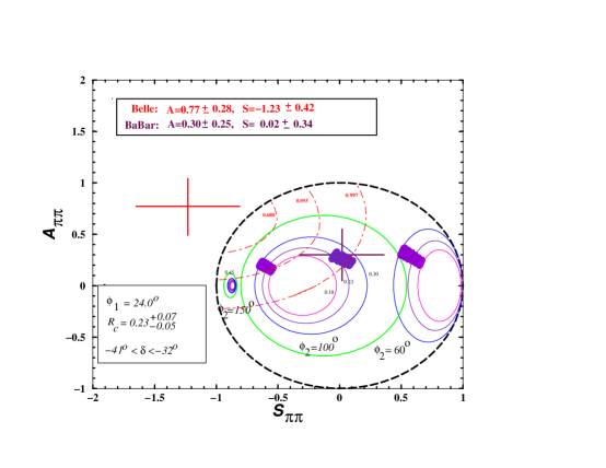
Figure 4: Correlation between $A_{\pi\pi}$ and $S_{\pi\pi}$ predicted by PQCD.

4 Recent Progress

4.1 $B$ meson wave function

The $B$ meson distribution amplitude, being the nonperturbative input for collinear factorization, is defined via the nonlocal matrix element,

$$\langle\,0\,|\,\bar{q}(y^{-})\,P\exp\left[-ig\int_{0}^{y^{-}}dzn_{-}\cdot A(zn_{-})\right]\,\Gamma\not n_{-}h(0)\,|\bar{B}(v)\rangle$$

$$\hskip 28.45274pt=-\frac{if_{B}\sqrt{m_{B}}}{2}{\tilde{\phi}}_{B}(y^{-},\mu)\,\mbox{tr}\left(\Gamma\not n_{-}\frac{1+\not v}{2}\,\gamma_{5}\right)\;,$$ (7)

where $n_{-}=(0,1,{\bf 0}_{T})$ is a null vector, $h$ the rescaled $b$ quark field characterized by the $B$ meson velocity $v$, $\mu$ the renormalization scale, and $\Gamma$ represents a Dirac matrix. The property of the $B$ meson distribution amplitude has been studied intensively in the literature [46, 47]. Especially, the asymptotic behavior of $\phi_{B}$ has been extracted from an evolution equation derived in the collinear factorization theorem [48].

Figure 5: Part of the $O(\alpha_{s})$ diagrams for $\phi_{B}$.

The analysis starts with the evaluation of the $O(\alpha_{s})$ diagrams in Fig. 6, which are drawn according to Eq. (4.1). Figures 6(a) and 6(b) give the correction,

$$Z^{(1)}_{ab}(k^{+},k^{\prime+},\mu) = -ig^{2}C_{F}\mu^{2\epsilon}\int\frac{d^{4-2\epsilon}l}{(2\pi)^{4-2\epsilon}}\frac{n_{-}\cdot v}{v\cdot ll^{2}n_{-}\cdot l}$$ (8)

$$\times\left[\delta(k^{+}-k^{\prime+})-\delta\left(k^{+}-k^{\prime+}+l^{+}\right)\right]\;.$$

The loop integral leads to the counterterm,

$$-\frac{\alpha_{s}C_{F}}{2\pi}{\frac{1}{\epsilon}}\left[\frac{k^{+}}{k^{\prime+}}\frac{\theta(k^{\prime+}-k^{+})}{(k^{\prime+}-k^{+})_{+}}+\frac{\theta(k^{+}-k^{\prime+})}{(k^{+}-k^{\prime+})_{+}}\right]\;,$$ (9)

where $1/\epsilon$ comes from the integration over $l_{T}$. The corresponding anomalous dimension, the splitting kernel, then determines the asymptotic behavior,

$${\phi_{B}(k^{+},\mu)\sim 1/k^{+}\;,\;\;{\rm for}\;\;k^{+}\to\infty}\;.$$ (10)

That is, the evolution effect ruins the normalizability of the $B$ meson distribution amplitude, and $f_{B}$ is not defined unambiguously. This feature has been confirmed in a QCD sum rule analysis [49].

Figure 6: The path of $s$.

Adopting $k_{T}$ factorization [50, 51], Eq. (4.1) is modified into

$$\langle 0|{\bar{q}}(y^{-},{b})P\exp\left[-ig\int_{0}^{(y^{-},{b})}ds\cdot A(s)\right]\Gamma\not n_{-}h(0)|{\bar{B}}(v)\rangle\;,$$ (11)

where the path of $s$ for the Wilson line consists of three pieces shown in Fig. 6. The Feynman rule for Figs. 6(a) and 6(b) is modified into

$$Z^{(1)}_{ab}(k^{+},k^{\prime+},b,\mu) = -ig^{2}C_{F}\mu^{2\epsilon}\int\frac{d^{4-2\epsilon}l}{(2\pi)^{4-2\epsilon}}\frac{n_{-}\cdot v}{v\cdot ll^{2}n_{-}\cdot l}$$ (12)

$$\times\left[\propto\delta(k^{+}-k^{\prime+})-\delta\left(k^{+}-k^{\prime+}+l^{+}\right){\exp(-i{\bf l}_{T}\cdot{\bf b})}\right]\;.$$

The extra Fourier factor $\exp(-i{\bf l}_{T}\cdot{\bf b})$ suppresses the large $l_{T}$ region, such that the integral is UV finite:

$$-\frac{\alpha_{s}C_{F}}{\pi}\left[\frac{\theta(k^{\prime+}-k^{+})}{(k^{\prime+}-k^{+})_{+}}K_{0}\left((k^{\prime+}-k^{+})b\right)-\frac{\theta(k^{+}-k^{\prime+})}{(k^{+}-k^{\prime+})_{+}}K_{0}\left((k^{+}-k^{\prime+})b\right)\right]\;.$$ (13)

Therefore, The evolution effect does not involve a splitting kernel, and does not change the $k^{+}$ distribution. The $B$ meson distribution amplitude is regarded as the small $b$ limit, $b\to 1/m_{B}\to 0$, of the $B$ meson wave function, at which the Bessel function $K_{0}$ remains UV finite. The above observation indicates that $k_{T}$ factorization is a more appropriate tool for exclusive $B$ meson decays than collinear factorization.

4.2 Radiative decays

The PQCD approach has been applied to radiative $B$ meson decays recently. We first summarize the experimental data for the $B\to K^{*}\gamma$ decays and the PQCD predictions [52] in Tables. 3 and 4, respectively, where the isospin breaking is defined as

$$\Delta_{0+} \equiv \frac{\Gamma(B^{0}\to K^{*0}\gamma)-\Gamma(B^{+}\to K^{*+}\gamma)}{\Gamma(B^{0}\to K^{*0}\gamma)+\Gamma(B^{+}\to K^{*+}\gamma)}\;.$$ (14)

Note that the large $B\to K^{*}\gamma$ branching ratios from NLO QCDF [53] just imply that the input form factor value $F^{BK^{*}}$ is too large [54, 55].

Quantities	Belle [56]	Babar [57]
$B(K^{*0}\gamma)(10^{-5})$	$4.01\pm 0.21\pm 0.17$	$3.92\pm 0.20\pm 0.24$
$B(K^{*\pm}\gamma)(10^{-5})$	$4.25\pm 0.31\pm 0.24$	$3.87\pm 0.28\pm 0.26$
$\mbox{A}_{CP}$	$-0.015\pm 0.044\pm 0.012$	$-0.013\pm 0.036\pm 0.010$
$\Delta_{0+}$	$+0.012\pm 0.044\pm 0.026$	$+0.051\pm 0.044\pm 0.023\pm 0.024$

Table 3: Data of the $B\to K^{*}\gamma$ decays.

Quantities	PQCD	QCDF
$B(K^{*0}\gamma)(10^{-5})$	$3.5^{+1.1}_{-0.8}$	7.4 ($\mu=m_{b}$)
$B(K^{*\pm}\gamma)(10^{-5})$	$3.4^{+1.2}_{-0.9}$
$\mbox{A}_{CP}$	$(0.39^{+0.06}_{-0.07})\%$	$0.3\%$
$\Delta_{0+}$	${+0.057^{+0.011}_{-0.013}}$	+0.038

Table 4: PQCD predictions for the $B\to K^{*}\gamma$ decays.

After determining the $B$ meson wave function $\phi_{B}$ from the $B\to\pi$ form factor, we can predict the above quantities in PQCD. We have considered the contributions from the operators ${O_{7\gamma}}$, ${O_{8g}}$, and $O_{2}$ (up and charm loops) and from the annihilation topology, and the long-distance contribution through the vector mesons. The theoretical errors for the branching ratios mainly come from the shape parameter in $\phi_{B}$, and those for the CP asymmetry mainly from the CKM parameters. It was found that the penguin annihilation from $O_{5,6}$ shown in Fig. 7 is the most important mechanism responsible for the positive isospin breaking.

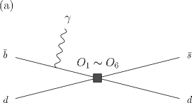
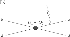
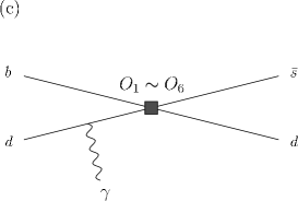
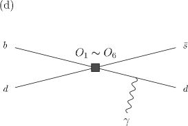
Figure 7: Annihilation diagrams from ${O_{1}\sim O_{6}}$.

We have also analyzed the $B\to\rho(\omega)\gamma$ decays. Preliminary PQCD predictions are listed in Table 5, and compared to those from QCDF. The small deviation between PQCDI and PQCDII is attributed to the different treatment of the long-distance contribution.

Branching ratio	Belle [58]	PQCDI [59]	PQCDII [60]	QCDF [61]
$B(\rho^{\pm}\gamma)$ ($10^{-6}$)	$1.8^{+0.8}_{-0.7}\pm 0.1$	2.1	$1.8^{+0.4}_{-0.5}$	1.6
$B(\rho^{0}\gamma)$ ($10^{-6}$)	$0.5^{+0.5}_{-0.4}\pm 0.2$	$0.95$	$0.9^{+0.3}_{-0.2}$	0.95
$B(\omega\gamma)$ ($10^{-6}$)	$1.3^{+0.7}_{-0.6}\pm 0.2$	$0.85$

Table 5: Branching ratios of the $B\to\rho(\omega)\gamma$ decays.

4.3 Polarizations in $VV$ modes

Pol. fraction	Belle [62, 63]	BaBar [64, 65, 66]
$R_{L}(\phi K^{*+})$		$0.46\pm 0.12\pm 0.03$
$R_{L}(\phi K^{*0})$	$0.43\pm 0.09\pm 0.04$	$0.52\pm 0.07\pm 0.02$
$R_{\perp}(\phi K^{*0})$	$0.41\pm 0.10\pm 0.02$	$0.27\pm 0.07\pm 0.02$
$R_{L}(\rho^{0}K^{*+})$		$0.96^{+0.04}_{-0.15}\pm 0.04$
$R_{L}(\rho^{0}\rho^{+})$	$0.95\pm 0.11\pm 0.02$	$0.97^{+0.03}_{-0.07}\pm 0.04$
$R_{L}(\rho^{+}\rho^{-})$		$0.98^{+0.02}_{-0.08}\pm 0.03$

Table 6: Polarization fractions in $B\to VV$ transitions.

The measured polarization fractions in $B\to VV$ modes are summarized in Table 6, whose implication will be discussed below. The power counting rules for the emission topologies are

$$R_{L}\sim 1\;,\;\;\;\;R_{\parallel}\sim R_{\perp}\sim O(m_{\phi}^{2}/m_{B}^{2})\;,$$ (15)

and those for the annihilation topologies from $O_{5,6}$ are

$${R_{L}\sim R_{\parallel}\sim R_{\perp}\sim O(m_{K^{*}}^{2}/m_{B}^{2},m_{\phi}^{2}/m_{B}^{2})}\;.$$ (16)

If the emission topologies dominate as expected, the $B\to\phi K^{*}$ data do not obey the counting rules obviously. If the annihilation contribution is enhanced by some mechanism, one could have $R_{L}\sim 0.5$. This is the strategy adopted in [67] based on QCDF.

I stress that any proposed mechanism has to explain all $VV$ modes simultaneously, especially $B\to\rho K^{*}$ [68], and that $B\to\phi K^{*}$ is so unique, since all other modes follow the expected counting rules. The annihilation amplitude is a free parameter in QCDF, since it involves the arbitrary end-point cutoff $\rho_{A}$. Because varying the free parameter to explain the data can not be conclusive, it is better to estimate the annihilation contribution in a reliable way. Viewing that the PQCD predictions for the annihilation amplitudes are consistent with the measured direct CP asymmetries in $B\to K\pi$, $\pi\pi$ [2, 3], this calculation has been performed in [69]. As shown in Table 7, the annihilation mechanism indeed helps, but is not sufficient to lower the fraction $R_{L}$ down to around 0.5.

A mechanism for enhancing the transverse polarization component in the $B\to\phi(\omega)K^{*}$ decays has been proposed in [70], which arises from the $b\to sg$ transition. The novelty is that the transverse polarization of the gluon from the transition propagates into the $\phi(\omega)$ meson, and that the constraint from the $B\to\rho K^{*}$ data is avoided. The relevant matrix element was then parameterized in terms of a dimensionless free parameter $\kappa$. By varying this parameter to $\kappa=-0.25$, the authors of [70] claimed that the $B\to\phi K^{*}$ data could be accommodated in the Standard Model. Our comment is that a reliable estimate of the $\kappa$ value is necessary. By means of the three-parton $\phi$ meson distribution amplitude and the naive factorization assumption, we have found that the order of magnitude of $\kappa$ is, unfortunately, 0.01. The detail will be supplied elsewhere.

Mode	$|A_{0}|^{2}$	$|A_{\parallel}|^{2}$	$|A_{\perp}|^{2}$	$\phi_{\parallel}(rad.)$	$\phi_{\perp}(rad.)$
$\phi K^{*0}$(I)	$0.923$	$0.040$	$0.035$	$\pi$	$\pi$
(II)	$0.860$	$0.072$	$0.063$	$3.30$	$3.33$
(III)	$0.833$	$0.089$	$0.078$	$2.37$	$2.34$
(IV)	$0.750$	$0.135$	$0.115$	$2.55$	$2.54$
$\phi K^{*+}$(I)	$0.923$	$0.040$	$0.035$	$\pi$	$\pi$
(II)	$0.860$	$0.072$	$0.063$	$3.30$	$3.33$
(III)	$0.830$	$0.094$	$0.075$	$2.37$	$2.34$
(IV)	$0.748$	$0.133$	$0.111$	$2.55$	$2.54$

Table 7: (I) Without nonfactorizable and annihilation contributions, (II) add only nonfactorizable contribution, (III) add only annihilation contribution, (IV) add both nonfactorizable and annihilation contributions.

4.4 New physics in $B\to\phi K_{S}$

It has been known that the discrepancy between the induced CP asymmetries $S_{J/\psi K_{S}}$ and $S_{\phi K_{S}}$ measured by Belle could be a possible new physics signal. The data of the $B\to\phi K_{s}$ mode are summarized below [71, 72]:

$$S_{J/\psi K_{S}} = \left\{\begin{array}[]{cl}0.741\pm 0.067\pm 0.034&(\mathrm{BaBar,\ 81\,fb}^{-1})\;,\\ 0.733\pm 0.057\pm 0.028&(\mathrm{Belle,\ 140\,fb}^{-1})\;,\\ \end{array}\right.$$

$$S_{\phi K_{S}} = \left\{\begin{array}[]{cl}0.45\pm 0.43\pm 0.07&\mathrm{(BaBar,\ 110\,fb}^{-1})\;,\\ {-0.96\pm 0.50\ {}^{+0.09}_{-0.11}}&\mathrm{(Belle,\ 140\,fb}^{-1})\;.\\ \end{array}\right.$$

There are already many works devoted to the new physics study in the above mode. Here I will not concentrate on the new physics effect, but on the advantage of exploring new physics in the PQCD framework.

It is expected that the new CP violating sources and the flavor changing neutral current in MSSM induce direct CP violations, and render $S_{\phi K_{S}}$ different from $S_{J/\psi K_{S}}$. Motivated by this observation, we have calculated the Wilson coefficients using the mass insertion approximation [34]. For example, the coefficient associated with the magnetic penguin operator is given by

$$C_{8G}^{\rm NP}(M_{S})\simeq\frac{\sqrt{2}\alpha_{s}\pi}{2G_{F}V_{ts}^{*}V_{tb}m_{\tilde{q}}^{2}}\left[(\delta_{LL}^{d})_{23}\left(\frac{1}{3}M_{3}(x)+\!3M_{4}(x)\right)+(\delta_{LR}^{d})_{23}\frac{m_{\tilde{g}}}{m_{b}}\left(\frac{1}{3}M_{1}(x)+3M_{2}(x)\right)\right]\;,$$ (19)

where $M_{S}$ is the SUSY scale, $x=m^{2}_{\tilde{g}}/m^{2}_{\tilde{q}}$ with $m_{\tilde{g}}$ and $m_{\tilde{q}}$ being the gluino and squark masses, respectively, and $B(x)$, $P(x)$ and $M(x)$ the loop functions from box and penguin diagrams [73, 74]. The relevant matrix element associated with $O_{8G}$ was then calculated in PQCD. Note that such a calculation is ambiguous in naive factorization because of the unknown gluon invariant mass $q^{2}$. In PQCD, it is written as $q^{2}=(1-x_{2})x_{3}M_{B}^{2}-|{\bf k}_{2T}-{\bf k}_{3T}|^{2}$ with $x_{2}$ and $k_{2T}$ ($x_{3}$ and $k_{3T}$) being the momentum fraction and the transverse momentum in the $K$ ($\phi$) meson.

Next step is to constrain the parameters $(\delta_{LL}^{d})_{23}$ $\cdots$ from the data of the branching ratio $B(B\to X_{s}\gamma)$ and of the $B_{s}-\overline{B_{s}}$ mixing, assuming $m_{\tilde{g}}=m_{\tilde{q}}=500$ GeV. The predicted range of $S_{\phi K_{S}}$ [34] is displayed in Fig. 8. One can further constrain the parameters from the $B\to\phi K$ branching ratios and direct CP asymmetries. Due to the larger strong phases, and the larger direct CP asymmetries from PQCD, one can extract a stronger constraint on new physics from the data. Conservatively, we have $S_{\phi K_{S}}\geq-0.28$ as exhibited in Fig. 8. Varying $m_{\tilde{g}}$ and $m_{\tilde{q}}$ arbitrarily, $S_{\phi K_{S}}$ reaches about $-40\%$. Therefore, it is difficult to explain the Belle data by the considered new physics.

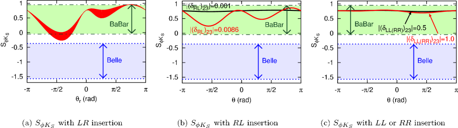
Figure 8: The result of $S_{\phi K_{S}}$ with the MSSM contribution. The dot-dashed (dotted) lines represent the $1\sigma$ error from BaBar (Belle).

5 Summary

In this talk I have summarized the recent progress on exclusive $B$ meson decays made in the PQCD approach based on $k_{T}$ factorization theorem. Both collinear and $k_{T}$ factorization theorems can be developed for these decays. In the former a heavy-to-light transition form factor exhibits an end-point singularity, while in the latter it is infrared-finite. Hence, soft dominance is postulated and a heavy-to-light form factor is parameterized as a nonperturbative input in collinear factorization. Hard dominance is postulated and a heavy-to-light form factor can be factorized into a convolution of a hard kernel with meson wave functions in $k_{T}$ factorization. Note that a mixed picture, in which soft and hard contributions are postulated to be of the same order of magnitude, has been proposed in SCET [25]. As explained above, there is no conflict between the soft-dominance and hard-dominance pictures for exclusive $B$ meson decays, which are due to the different theoretical frameworks. The $B\to\pi$ form factor $F^{B\pi}$ is not factorizable, partially factorizable, and completely factorizable in QCDF, SCET, and PQCD, respectively.

It has been found that the evolution of the $B$ meson distribution amplitude in collinear factorization ruins its normalizability, while the evolution of the $B$ meson wave function in $k_{T}$ factorization is well-behaved. The branching ratios, CP asymmetries, and isospin breaking in radiative decays have been calculated. The results are consistent with the data. The annihilation contribution can be estimated in PQCD reliably. Its effect helps, but is not sufficient for explaining the observed $B\to\phi K^{*}$ polarization fractions. We have taken the induced CP asymmetry in the $B\to\phi K_{S}$ mode as an example to demonstrate that PQCD gives a stronger constraint on new physics [75].

I did not cover the following subjects in this talk: the evaluation of the nonfactorizable contribution to the decays $B\to D^{(*)}\pi(\rho,\omega)$ [76], the analysis of three-body decays by means of two-meson distribution amplitudes [77], and the studies of decays into scalar mesons [78].

I thank the KTPQCD group members for useful comments and discussions. This work was supported in part by the National Science Council of R.O.C. under Grant No. NSC-92-2112-M-001-030 and by Taipei branch of the National Center for Theoretical Sciences of R.O.C..

References

- [1] H-n. Li and H.L. Yu, Phys. Rev. Lett. 74, 4388 (1995); Phys. Lett. B 353, 301 (1995); Phys. Rev. D 53, 2480 (1996).
- [2] Y.Y. Keum, H-n. Li, and A.I. Sanda, Phys. Lett. B 504, 6 (2001); Phys. Rev. D 63, 054008 (2001); Y.Y. Keum and H-n. Li, Phys. Rev. D63, 074006 (2001).
- [3] C. D. Lü, K. Ukai, and M. Z. Yang, Phys. Rev. D 63, 074009 (2001).
- [4] M. Beneke, G. Buchalla, M. Neubert, and C.T. Sachrajda, Phys. Rev. Lett. 83, 1914 (1999); Nucl. Phys. B591, 313 (2000).
- [5] C.W. Bauer, S. Fleming, and M. Luke, Phys. Rev. D 63, 014006 (2001).
- [6] C.W. Bauer, S. Fleming, D. Pirjol, and I.W. Stewart, Phys. Rev. D 63, 114020 (2001).
- [7] V.L. Chernyak and I.R. Zhitnitsky, Nucl. Phys. B345, 137 (1990).
- [8] A. Ali, V.M. Braun, and H. Simma, Z. Phys. C 63, 437 (1994).
- [9] A. Khodjamirian, Nucl. Phys. B605, 558 (2001).
- [10] C.Y. Cheung, W.M. Zhang, and G.L. Lin, Phys. Rev. D 52, 2915 (1995).
- [11] H.M. Choi and C.R. Ji, Phys. Lett. B 460, 461 (1999).
- [12] G. Sterman, An Introduction to Quantum Field Theory, Cambridge, 1993.
- [13] S. Catani, M. Ciafaloni and F. Hautmann, Phys. Lett. B 242, 97 (1990); Nucl. Phys. B366, 135 (1991).
- [14] J.C. Collins and R.K. Ellis, Nucl. Phys. B360, 3 (1991).
- [15] E.M. Levin, M.G. Ryskin, Yu.M. Shabelskii, and A.G. Shuvaev, Sov. J. Nucl. Phys. 53, 657 (1991).
- [16] G.P. Lepage and S.J. Brodsky, Phys. Lett. B 87, 359 (1979); Phys. Rev. D 22, 2157 (1980).
- [17] A.V. Efremov and A.V. Radyushkin, Phys. Lett. B 94, 245 (1980).
- [18] V.L. Chernyak, A.R. Zhitnitsky, and V.G. Serbo, JETP Lett. 26, 594 (1977).
- [19] V.L. Chernyak and A.R. Zhitnitsky, Sov. J. Nucl. Phys. 31, 544 (1980); Phys. Rep. 112, 173 (1984).
- [20] J. Botts and G. Sterman, Nucl. Phys. B225, 62 (1989).
- [21] H-n. Li and G. Sterman, Nucl. Phys. B381, 129 (1992).
- [22] H-n. Li, Phys. Rev. D 64, 014019 (2001); M. Nagashima and H-n. Li, hep-ph/0202127.
- [23] A. Szczepaniak, E.M. Henley, and S. Brodsky, Phys. Lett. B 243, 287 (1990).
- [24] M. Beneke and T. Feldmann, Nucl. Phys. B592, 3 (2000).
- [25] C.W. Bauer, D. Pirjol, and I.W. Stewart, Phys. Rev. D 67, 071502 (2003); R.J. Hill, T. Becher, S.J. Lee, and M. Neubert, hep-ph/0404217.
- [26] C.W. Bauer, D. Pirjol, I.Z. Rothstein, and I.W. Stewart, hep-ph/0401188.
- [27] T. Kurimoto, H-n. Li, and A.I. Sanda, Phys. Rev. D 65, 014007 (2002).
- [28] J.C. Collins, Acta. Phys. Polon. B 34, 3103 (2003).
- [29] S. Descotes-Genon and C.T. Sachrajda, Nucl. Phys. B625, 239 (2002).
- [30] Z.T. Wei and M.Z. Yang, Nucl. Phys. B642, 263 (2002); C.D. Lu and M.Z. Yang, Eur. Phys. J. C 28, 515 (2003).
- [31] N. Mahajan, hep-ph/0405161.
- [32] C.H. Chen, Y.Y. Keum, and H-n. Li, Phys. Rev. D 64, 112002 (2001).
- [33] S. Mishima, Phys. Lett. B 521, 252 (2002).
- [34] S. Mishima and A.I. Sanda, Phys. Rev. D 69, 054005 (2004).
- [35] H.Y. Cheng and K.C. Yang, Phys. Rev. D 64, 074004 (2001).
- [36] X.G. He, J.P. Ma, and C.Y. Wu, Phys. Rev. D 63, 094004 (2001).
- [37] D. Du, J. Sun, D. Yang, and G. Zhu, Phys. Rev. D 67, 014023 (2003).
- [38] M. Beneke and M. Neubert, hep-ph/0308039.
- [39] P. Ball and M. Boglione, Phys. Rev. D 68, 094006 (2003).
- [40] Y. Chao et al., [Belle Collaboration], hep-ex/0407025.
- [41] B. Aubert et al. [BABAR Collaboration], hep-ex/0407057.
- [42] K. Abe et al., [Belle Collaboration], Phys. Rev. Lett. 93, 021601 (2004).
- [43] B. Aubert et al. [BABAR Collaboration], Phys. Rev. Lett. 89, 281802 (2002).
- [44] Y.Y. Keum, H-n. Li, and A.I. Sanda, AIP Conf. Proc. 618, 229 (2002); Y.Y. Keum and A.I. Sanda, Phys. Rev. D 67, 054009 (2003).
- [45] M. Beneke, hep-ph/0207228.
- [46] A.G. Grozin and M. Neubert, Phys. Rev. D 55, 272 (1997).
- [47] H. Kawamura, J. Kodaira, C.F. Qiao, and K. Tanaka, Phys. Lett. B 5 23, 111 (2001); Erratum-ibid. 536, 344 (2002); Mod. Phys. Lett. A 18, 799 (2003).
- [48] B.O. Lange and M. Neubert, Phys. Rev. Lett. 91, 102001 (2003).
- [49] V.M. Braun, D.Yu. Ivanov, G.P. Korchemsky, Phys. Rev. D 69, 034014 (2004).
- [50] M. Nagashima and H-n. Li, Phys. Rev. D 67, 034001 (2003).
- [51] H-n. Li and H.S. Liao, hep-ph/0404050.
- [52] Y.Y. Keum, M. Matsumori, and A.I. Sanda, hep-ph/0406055.
- [53] S.W. Bosch and G. Buchalla, Nucl. Phys. B621, 459 (2002).
- [54] A. Ali, hep-ph/0210183.
- [55] H.Y. Cheng and C.K. Chua, Phys. Rev. D 69, 094007 (2004).
- [56] M. Nakao et al. [Belle Collaboration], Phys. Rev. D 69, 112001 (2004).
- [57] P. Tan et al. [BABAR Collaboration], APS Meeting, April 2004.
- [58] M. Iwasaki [Belle Collaboration], hep-ex/0406059.
- [59] C.D. Lu, M. Matsumori, A.I. Sanda, and M.Z. Yang, in preparation.
- [60] A. Ali and Y.Y. Keum, in preparation.
- [61] S.W. Bosch, hep-ph/0208204.
- [62] K.F. Chen et al. [Belle Collaboration], Phys. Rev. Lett. 91, 201801 (2003).
- [63] J. Zhang et al. [BELLE Collaboration], Phys. Rev. Lett. 91, 221801 (2003).
- [64] B. Aubert et al. [BABAR Collaboration], Phys. Rev. Lett. 91, 171802 (2003).
- [65] B. Aubert et al. [BABAR Collaboration], Phys. Rev. D 69, 031102 (2004).
- [66] A. Gritsan, talk given at LBNL, April 2004, BaBar-COLL-0028.
- [67] A.L. Kagan, hep-ph/0405134.
- [68] P. Colangelo, F. De Fazio, and T.N. Pham, hep-ph/0406162.
- [69] C.H. Chen, Y.Y. Keum, and H-n. Li, Phys. Rev. D 66, 054013 (2002).
- [70] W.S. Hou and M. Nagashima, hep-ph/0408007.
- [71] B. Aubert et al. [BABAR Collaboration], Phys. Rev. Lett. 89, 201802 (2002).
- [72] K. Abe et al. [Belle Collaboration], hep-ex/0308036.
- [73] F. Gabbiani, E. Gabrielli, A. Masiero, and L. Silvestrini, Nucl. Phys. B477, 321 (1996).
- [74] R. Harnik, D.T. Larson, H. Murayama, and A. Pierce, Phys. Rev. D 69, 094024 (2004).
- [75] S. Nandi and A. Kundu, hep-ph/0407061.
- [76] Y.Y. Keum, T. Kurimoto, H.-n. Li, C.D. Lu, and A.I. Sanda, Phys. Rev. D 69, 094018 (2004).
- [77] C.H. Chen and H-n. Li, Phys. Lett. B 561, 258 (2003); hep-ph/0404097.
- [78] C.H. Chen, Phys. Rev. D 67, 094011 (2003); Phys. Rev. D 68, 114008 (2003).