Baryon structure in a quark-confining non-local NJL model

Abstract

We study the nucleon and diquarks in a non-local Nambu-Jona-Lasinio model. For certain parameters the model exhibits quark confinement, in the form of a propagator without real poles. After truncation of the two-body channels to the scalar and axial-vector diquarks, a relativistic Faddeev equation for nucleon bound states is solved in the covariant diquark-quark picture. The dependence of the nucleon mass on diquark masses is studied in detail. We find parameters that lead to a simultaneous reasonable description of pions and nucleons. Both the diquarks contribute attractively to the nucleon mass. Axial-vector diquark correlations are seen to be important, especially in the confining phase of the model. We study the possible implications of quark confinement for the description of the diquarks and the nucleon. In particular, we find that it leads to a more compact nucleon.

I Introduction

The NJL model is a successful phenomenological field theory inspired by QCD njl . The model is constructed to obey the basic symmetries of QCD in the quark sector, but unlike the case of low-energy QCD, quarks are not confined. The basic ingredient of the model is a zero-range interaction containing four fermion fields. This means that the model is not renormalizable. Therefore at one-loop level an ultraviolet cut-off supplemented with a regularization method is required from the outsets. The value of the cut-off can be related to the scale of physical processes not included in the model, and thus determines its range of validity. Consequently, processes involving a large momentum transfer can not be described by the model. At higher orders in the loop expansion, which are necessary for calculating mesonic (baryonic) fluctuations njl-cut ; cut-b , one needs extra cut-off parameters. It is hard to determine these parameters from independent physics, and thus to build a viable phenomenology. A similar problem appears in the diquark-quark picture of baryons where an additional cut-off parameter is required to regularise the diquark-quark loops cut-b .

Another drawback of the model is the absence of confinement, which makes it questionable for the description of few-quark states and for quark matter. If energetically allowed, the mesons of the model can decay into free quark-antiquark pairs, and the presence of unphysical channels is another limitation on the applicability of NJL model. At the same time, it is also known that the NJL model exhibits a zero-temperature phase transition at unrealistically low baryon density njl-ma . This problem is caused by the formation of unphysical coloured diquark states. These may be explicitly excluded at zero density by a projection onto the physical channels, but dominate the behaviour at finite density. The model is not able to describe nuclear matter, even in the low-density regime w .

We do not know how to implement colour confinement in the model and, anyway, the exact confining mechanism of QCD is still unknown. In the context of an effective quark theory, a slightly different mechanism of “quark confinement” can be described by a quark propagator which vanishes due to infra-red singularities rho2 or which does not produce any poles corresponding to asymptotic quark states rho1 ; asy . Another realisation of quark confinement can be found in Ref. rho . It has been shown that a non-local covariant extension of the NJL model inspired by the instanton liquid model non1 can lead to quark confinement for acceptable values of the parameters pb . This model has previously been applied to mesons pb ; pb-2 ; a1 and in this paper it is applied to baryons based on the relativistic Faddeev approach.

The quark propagator in the model has no real pole and consequently quarks do not appear as asymptotic states. Instead the quark propagator has pairs of complex poles. This phenomenon was also noticed in Schwinger-Dyson equation studies in QED and QCD sde-p ; sde-new ; sde-qe . One can simply accept the appearance of these poles as an artifact of the naive truncation scheme involved. However, it has been recently suggested that it might be a genuine feature of the full theory, and be connected with the underlying confinement mechanism sde-new ; sde-qe . For example, it has been shown by Maris that if one removes the confining potential in QED in 2+1D the mass singularities are located almost on the time axis, and if there is a confining potential, the mass-like singularities move from the time axis to complex momenta sde-qe . In this paper, we study this kind of confinement from another viewpoint. We show that when we have quark confinement in the non-local NJL model, the baryons become more compact, compared to a situation where we have only real poles for quark propagator.

There are several other advantages of the non-local version of the model over the local NJL model: the dynamical quark mass is momentum-dependent, as also found in lattice simulations of QCD lat-m . There various methods are available for construction of a conserved current in the presence of non-local interactions non-j . In general, one can preserve the gauge invariance and anomalies by introducing additional non-local terms in the currents non-j . A Noether-like method of construction for these non-local pieces for the non-local NJL model was developed in Ref. pb . The regulator makes the theory finite to all orders in the loop expansion and leads to small next-to-leading order corrections pb-2 . As a result, the non-local version of the NJL model should have more predictive power.

We use a separable non-local interactions, similar to that of the instanton-liquid model non1 ; sep-i . This considerably simplifies the calculation. Other approaches also give non-locality but in different forms asy ; non-bir . Non-locality also emerges naturally in the Schwinger-Dyson resummation asy and in various types of gluonic field configuration within the QCD vacuum, see for an example Ref. gluon .

Considerable work has been done on these nonlocal NJL models including applications to the mesonic sector pb ; pb-2 ; a1 , phase transitions at finite temperature and densities a2 , and the study of chiral solitons a3 .

In this paper we present our first results from a calculation of the relativistic Faddeev equation for a non-local NJL model, based on the covariant diquark-quark picture of baryons njln1 ; njln2 ; njln3 ; njln4-is ; njln4 ; o1 ; o2 ; o3 ; o4 . Such an approach has been extensively employed to study baryons in the local NJL model, see, e.g., Refs. njln1 ; njln2 ; njln3 ; njln4-is ; njln4 . We include both scalar and the axial-vector diquark correlations. We do not assume a special form for the interaction Lagrangian, but we rather treat the coupling in the diquark channels as free parameters and consider the range of coupling strengths which lead to a reasonable description of the nucleon. We construct diquark and nucleon solutions and study the possible implications of the quark confinement for the solutions. The dependence of the baryon masses and waves on the diquarks parameters is investigated and the role of diquarks in the nucleon solutions, for both the confining and the non-confining phase of the model is considered separately. The nucleon wave function is studied in details. Due to the separability of the non-local interaction, the Faddeev equations can be reduced to a set of effective Bethe-Salpeter equations. This makes it possible to adopt the numerical method developed for such problems in Refs. o1 ; o2 ; o3 ; o4 .

This paper is organised as follows: In Sec. II the model is introduced. We also discuss the pionic sector of the model and fix the parameters. In Sec. III the diquark problem is solved and discussed. In Sec. IV the three-body problem based on diquark-quark picture is investigated. The numerical technique involved in solving the effective Bethe-Salpeter equation is given and the results for three-body sector are presented. Finally, a summary and outlook is given in Sec. V.

II A non-local NJL model

We consider a non-local NJL model Lagrangian with $SU(2)_{f}\times SU(3)_{c}$ symmetry.

$$\mathcal{L}=\bar{\psi}(i\partial\kern-4.49997pt/-m_{c})\psi+\mathcal{L}_{I},$$ (1)

where $m_{c}$ is the current quark mass of the $u$ and $d$ quarks and $\mathcal{L}_{I}$ is a chirally invariant non-local interaction Lagrangian. Here we restrict the interaction terms to four-quark interaction vertices.

There exist several versions of such non-local NJL models. Regardless of what version is chosen, by a Fierz transformation one can rewrite the interaction in either the quark-antiquark or quark-quark channels. We therefore use the interaction strengths in those channels as independent parameters. For simplicity we truncate the mesonic channels to the scalar ($0^{+},T=0$) and pseudoscalar ($0^{-},T=1$) ones. The quark-quark interaction is truncated to the scalar ($0^{+},T=0$) and axial vector ($1^{+},T=1$) colour $\overline{3}$ quark-quark channels (the colour $6$ channels do not contribute to the colourless three-quark state considered here). We parametrise the relevant part of interaction Lagrangian as

$$\mathcal{L}_{I} = \frac{1}{2}g_{\pi}j_{\alpha}(x)j_{\alpha}(x)+g_{s}\overline{J}_{s}(x)J_{s}(x)+g_{a}\overline{J}_{a}(x)J_{a}(x),$$

$$j_{\alpha}(x) = \int d^{4}x_{1}d^{4}x_{3}F(x-x_{3})F(x_{1}-x)\overline{\psi}(x_{1})\Gamma_{\alpha}\psi(x_{3}),$$

$$\overline{J}_{s}(x) = \int d^{4}x_{1}d^{4}x_{3}F(x-x_{3})F(x_{1}-x)\overline{\psi}(x_{1})\big{[}\gamma_{5}C\tau_{2}\beta^{A}\big{]}\overline{\psi}^{T}(x_{3}),$$

$$J_{s}(x) = \int d^{4}x_{2}d^{4}x_{4}F(x-x_{4})F(x_{2}-x)\psi^{T}(x_{2})\big{[}C^{-1}\gamma_{5}\tau_{2}\beta^{A}\big{]}\psi(x_{4}),$$

$$\overline{J}_{a}(x) = \int d^{4}x_{1}d^{4}x_{3}F(x-x_{3})F(x_{1}-x)\overline{\psi}(x_{1})\big{[}\gamma_{\mu}C\tau_{i}\tau_{2}\beta^{A}\big{]}\overline{\psi}^{T}(x_{3}),$$

$$J_{a}(x) = \int d^{4}x_{2}d^{4}x_{4}F(x-x_{4})F(x_{2}-x)\psi^{T}(x_{2})\big{[}C^{-1}\gamma^{\mu}\tau_{2}\tau_{i}\beta^{A}\big{]}\psi(x_{4}),\$$ (2)

where $\Gamma_{\alpha}=(1,i\gamma_{5}\tau)$. The matrices $\beta^{A}=\sqrt{3/2}\lambda^{A}(A=2,5,7)$ project onto the colour $\overline{3}$ channel with normalisation $\operatorname{tr}(\beta^{A}\beta^{A^{\prime}})=3\delta^{AA^{\prime}}$ and the ${\tau_{i}}$’s are flavour $SU(2)$ matrices with $\operatorname{tr}(\tau_{i}\tau_{j})=2\delta_{ij}$. The object $C=i\gamma_{2}\gamma_{5}$ is the charge conjugation matrix. It is exactly this four-way separability of the non-local interaction that is also present in the instanton liquid model sep-i .

Since we do not restrict ourselves to a specific choice of underlying interaction, we shall treat the couplings $g_{s}$, $g_{a}$ and $g_{\pi}$ as independent parameters. We assume $g_{\pi,s,a}>0$, which leads to attraction in the given channels (and repulsion in the quark-antiquark colour octet and quark-quark colour antisextet channels). The coupling parameter $g_{\pi}$ is responsible for the pions and their isoscalar partner $\sigma$. The coupling strengths $g_{s}$ and $g_{a}$ specify the behaviour in the scalar and axial-vector diquark channel, respectively.

We define the Fourier transform of the form factor by

$$F(x-x_{i})=\int\frac{d^{4}p}{(2\pi)^{4}}e^{-i(x-x_{i})\cdot p}f(p).$$ (3)

The dressed quark propagator $S(k)$ is now constructed by means of a Schwinger-Dyson equation (SDE) in the rainbow-ladder approximation. Thus the dynamical constituent quark mass, arising from spontaneously broken chiral symmetry, is obtained in Hartree approximation as

$$m(p)=m_{c}+ig_{\pi}f^{2}(p)\int\frac{d^{4}k}{(2\pi)^{4}}\operatorname{Tr}[S(k)]f^{2}(k),$$ (4)

where

$$S^{-1}(k)=k\kern-4.49997pt/-m(k).$$ (5)

One can simplify this equation by writing $m(p)$ in the form

$$m(p)=m_{c}+(m(0)-m_{c})f^{2}(p).$$ (6)

The non-linear equation can then be solved iteratively for $m(0)$.

Following Ref. pb , we choose the form factor to be Gaussian in Euclidean space, $f(p_{E})=\exp(-p_{E}^{2}/\Lambda^{2})$, where $p_{E}$ denotes the Euclidean four-momentum and $\Lambda$ is a cutoff of the theory. This choice respects Poincaré invariance and for certain values of the parameters it leads to quark, but not colour, confinement. For values of $m(0)$ satisfying

$$\frac{m(0)-m_{c}}{\sqrt{m^{2}_{c}+\Lambda^{2}}-m_{c}}>\frac{1}{2}\exp\left(-\frac{(\sqrt{m^{2}_{c}+\Lambda^{2}}+m_{c})^{2}}{2\Lambda^{2}}\right),$$ (7)

the dressed quark propagator has no poles at real $p^{2}$ in Minkowski space ($p^{2}+m^{2}(p^{2})\neq 0$). The propagator has many pairs of complex poles, both for confining and non-confining parameter sets. This is a feature of these models and due care should be taken in handling such poles, which can not be associated with asymptotic states if the theory is to satisfy unitarity. One should note that the positions of these poles depend on the details of the chosen form factor and the cut-off, hence one may regard them as a pathology of the regularisation scheme. Since the choice of the cut-off is closely related to the truncation of the mesonic channels, (for example, if one allows mixing of channels, the cut-off and the positions of poles will change). Even though the confinement in this model has no direct connection to the special properties of the pion, there is an indirect connection through the determination of the parameters from the pionic properties.

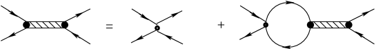
Figure 1: A graphical representation of the Bethe-Salpeter equation for the $\bar{q}q$ $T$-matrix in RPA approximation. The solid lines denote the dressed quark propagators Eq. (5) and shaded boxes denote meson propagators.

Figure 2: One-pion-to-vacuum matrix element in RPA, contributing to the weak pion decay. The lines are as defined in Fig. 1. The wavy line denotes a weak decay.

The quark-antiquark $T$-matrix in the pseudoscalar channel can be solved by using the Bethe-Salpeter equation in the random phase approximation (RPA), as shown in Fig. 1, see Ref. pb .

$$T(p_{1},p_{2},p_{3},p_{4}) = f(p_{1})f(p_{2})\big{[}i\gamma_{5}\tau_{i}\big{]}\frac{g_{\pi}i}{1+g_{\pi}J_{\pi}(q^{2})}\big{[}i\gamma_{5}\tau_{i}\big{]}f(p_{3})f(p_{4})$$ (8)

$$\times\delta(p_{1}+p_{2}-p_{3}-p_{4}),\$$

where

$$J_{\pi}(q^{2}) = i\operatorname{Tr}\int\frac{d^{4}k}{(2\pi)^{4}}f^{2}(k)\gamma_{5}\tau_{i}S(k)\gamma_{5}\tau_{i}S(q+k)f^{2}(q+k),$$ (9)

$$= 6i\int\frac{d^{4}k}{(2\pi)^{4}}\operatorname{tr}_{D}[\gamma_{5}S(k)\gamma_{5}S(k+q)]f^{2}(k)f^{2}(q+k),\$$

where $q$ denotes the total momentum of the quark-antiquark pair. The pion mass $m_{\pi}$ corresponds to the pole of $T$-matrix. One immediately finds that $m_{\pi}=0$ if the current quark mass $m_{c}$ is zero, in accordance with Goldstone’s theorem. The residue of the $T$-matrix at this pole has the form

$$V^{\pi}(p_{1},p_{2})=ig_{\pi qq}[\openone_{c}\otimes\tau^{a}\otimes\gamma_{5}]f(p_{1})f(p_{2}),$$ (10)

where $g_{\pi qq}$ is the pion-quark-antiquark coupling constant and is related to the corresponding loop integral $J_{\pi}$ by

$$g^{-2}_{\pi qq}=\left.\frac{dJ_{\pi}}{dq^{2}}\right|_{q^{2}=m^{2}_{\pi}}.$$ (11)

Table 1: The parameters for the sets $A$ and $B$, fitted to $f_{\pi}=92.4$ MeV and $m_{\pi}=139.6$ MeV. The resulting values of the dynamical quark mass $m(0)$ are also shown.

Parameter	set A	set B
$m(0)$ (MeV)	297.9	351.6
$m_{0}(0)$ (MeV)	250	300
$m_{c}$ (MeV)	7.9	11.13
$\Lambda$ (MeV)	1046.8	847.8
$g_{\pi}(\text{GeV}^{-2})$	31.6	55.80

Table 2: The first two sets of poles of the quark propagator (in magnitude) in the Minkowski frame.

set A	set B
$\pm 391$ MeV	$\pm 408\pm 238i$ MeV
$\pm 675$ MeV	$\pm 1575\pm 307i$ MeV

The pion decay constant $f_{\pi}$ is obtained from the coupling of the pion to the axial-vector current. Notice that due to the non-locality the axial-vector current is modified pb ; non-j and consequently the one-pion-to-vacuum matrix element gets the additional contribution shown in Fig. 2. This extra term is essential in order to maintain Gell-Mann-Oakes-Renner relation pb and makes a significant contribution. The pion decay constant is given by

$$f_{\pi} = \frac{ig_{\pi\bar{q}q}}{m_{\pi}^{2}}\int\frac{d^{4}k}{(2\pi)^{4}}\operatorname{Tr}[q\kern-4.49997pt/\gamma_{5}\frac{\tau_{a}}{2}(S(p_{-}))\gamma_{5}\tau_{a}(S(p_{+}))]f(p_{-})f(p_{+})$$ (12)

$$+ \frac{ig_{\pi}}{2m^{2}_{\pi}}\int\frac{d^{4}k}{(2\pi)^{4}}\operatorname{Tr}[S(k)]\int\frac{d^{4}k}{(2\pi)^{4}}\operatorname{Tr}[V^{\pi}(p_{-},p_{+})S(p_{-})\gamma_{5}\tau_{a}S(p_{+})]$$

$$\times[f^{2}(k)\left(f^{2}(p_{+})+f^{2}(p_{-})\right)-f(p_{+})f(p_{-})f(k)\left(f(k+q)+f(k-q)\right)],\$$

where $V_{\pi}(p_{-},p_{+})$ is defined in Eq. (10), with the notation $p_{\pm}=p\pm\frac{1}{2}q$.

The loop integrations in Eqs. (9,12) are evaluated in Euclidean space. For the current model, the usual analytic continuation of amplitudes from Euclidean to Minkowski space can not be used. This is due to the fact that quark propagators of the model contain many poles at complex energies leading to opening of a threshold for decay of a meson into other unphysical states. Any theory of this type needs an alternative continuation prescription consistent with unitarity and macrocausality. Let us define a fictitious two-body threshold as twice the real part of the first pole of the dressed quark propagator $m^{\text{q}}_{R}$. For a confining parameter set, each quark propagator has a pair of complex-conjugate poles. Above the two-body pseudo-threshold $q^{2}<-4(m^{\text{q}}_{R})^{2}$, where $q$ is the meson momentum, the first pair of complex poles of the quark propagator has a chance to cross the real axis. According to the Cutkosky prescription cutk , if one is to preserve the unitarity and the microcausality, the integration contour should be pinched at that point. In this way, one can ensure that there is no spurious quark-antiquark production threshold, for energies below the next pseudo-threshold, i.e. twice the real part of the second pole of the quark propagator. Note that it has been shown u that the removal of the quark-antiquark pseudo-threshold is closely related to the existence of complex poles in the form of complex-conjugate pairs. Since there is no unique analytical continuation method available for such problems, any method must be regarded as a part of the model assumptions pb ; a1 ; u . Here, we follow the method used in Ref. pb .

Our model contains five parameters: the current quark mass $m_{c}$, the cutoff ($\Lambda$), the coupling constants $g_{\pi}$ , $g_{s}$ and $g_{a}$. We fix the first three to give a pion mass of $m_{\pi}=139.6$ MeV with decay constant $f_{\pi}=92.4$ MeV, while we take the value of the zero-momentum quark mass in the chiral limit $m_{0}(0)$ as an input. We analyse two sets of parameters, as indicated in Table 1, where set $A$ is a non-confining parameter set, while set $B$ leads to quark confinement (i.e., it satisfies the condition Eq. (7)). The position of the quark poles are given in Table 2. The real part of the first pole of the dressed quark propagator $m^{\text{q}}_{R}$ can be considered in much the same as the quark mass in the ordinary NJL model. Since we do not believe in on-shell quarks or quark resonances, this is also a measure for a limit on the validity of the theory. The mass $m^{\text{q}}_{R}$ is larger than the constituent quark mass at zero momentum $m(0)$, as can be seen in Table 1. As we will see $m^{\text{q}}_{R}$ appears as an important parameter in the diquark and nucleon solution, rather than the constituent quark mass. The same feature has been seen in the studies of the soliton in this model, where $m^{\text{q}}_{R}$ determines the stability of the soliton a3 . The parameters $g_{s}$ and $g_{a}$ will be treated here as free parameters, which allows us to analyse baryon solutions in terms of a complete set of couplings. This is permissible as long as the interactions in Lagrangian are not fixed by some underlying theory via a Fierz transformation. The coupling-constant dependence is expressed through the ratios $r_{s}=g_{s}/g_{\pi}$ and $r_{a}=g_{a}/g_{\pi}$.

The quark condensate $\langle\bar{\psi}\psi\rangle=i\operatorname{Tr}S(0)$ is closely related to the gap equation, Eq. (4). In the latter there appears an extra form factor inside the loop integral. The quark condensate in the chiral limit is $-(207\text{ MeV})^{3}$ and $-(186\text{ MeV})^{3}$ for sets A and B, respectively. These values fall within the limits extracted from QCD sum rules qcdsum and lattice calculations lat-con , having in mind that QCD condensate is a renormalised and scale-dependent quantity. In contrast to the local NJL model, here the dynamical quark mass Eq. (6) is momentum dependent and follows a trend similar to that estimated from lattice simulations lat-m .

III Diquark channels

In the rainbow-ladder approximation the scalar quark-quark $T$-matrix can be calculated from a very similar diagram to that shown in Fig. 1 (the only change is that the anti-quark must be replaced by a quark with opposite momentum). It can be written as

$$T(p_{1},p_{2},p_{3},p_{4}) = f(p_{1})f(p_{2})\big{[}\gamma_{5}C\tau_{2}\beta^{A}\big{]}\tau(q)\big{[}C^{-1}\gamma_{5}\tau_{2}\beta^{A}\big{]}f(p_{3})f(p_{4})$$ (13)

$$\times\delta(p_{1}+p_{2}-p_{3}-p_{4}),\$$

with

$$\tau(q)=\frac{2g_{s}i}{1+g_{s}J_{s}(q^{2})},$$ (14)

where $q=p_{1}+p_{2}=p_{3}+p_{4}$ is the total momentum of the quark-quark pair, and

$$J_{s}(q^{2}) = i\operatorname{Tr}\int\frac{d^{4}k}{(2\pi)^{4}}f^{2}(-k)\big{[}\gamma_{5}C\tau_{2}\beta^{A}\big{]}S(-k)^{T}\big{[}C^{-1}\gamma_{5}\tau_{2}\beta^{A}\big{]}S(q+k)f^{2}(q+k),$$ (15)

$$= 6i\int\frac{d^{4}k}{(2\pi)^{4}}\operatorname{tr}_{D}[\gamma_{5}S(k)\gamma_{5}S(k+q)]f^{2}(k)f^{2}(q+k).$$

In the above equation the quark propagator $S(k)$ is the solution of the rainbow SDE Eq. (5). The denominator of Eq. (14) is the same as in the expression for the pion channel, Eq. (8), if $g_{s}=g_{\pi}$. One may thus conclude that at $r_{s}=1$ the diquark and pion are degenerate. This puts an upper limit to the choice of $r_{s}$, since diquarks should not condense in vacuum. One can approximate $\tau(q)$ by an effective diquark “exchange” between the external quarks, and parametrise $\tau(q)$ near the pole as

$$\tau(q)=2ig^{2}_{dsqq}V^{s}(q)D(q),\hskip 56.9055ptD^{-1}(q)=q^{2}-M^{2}_{ds},$$ (16)

where $M_{ds}$ is the scalar diquark mass, defined as the position of the pole of $\tau(q)$. The strength of the on-shell coupling of scalar diquark to quarks, $g_{dsqq}$ is related to the polarisation $J_{s}$ by

$$g^{-2}_{dsqq}=\frac{dJ_{s}}{dq^{2}}|_{q^{2}=M^{2}_{ds}},$$ (17)

and $V^{s}(q)$ is the ratio between the exact $T$-matrix and on-shell (one-pole) approximation and describes the off-shell correction of the $T$-matrix around the diquark solutions off-shell-d . For the “on-shell approximation” we have $V^{s}(q)=1$ njl ; cut-b , and by definition on the mass shell $q^{2}=M^{2}_{ds}$, one has $V^{s}(q)|_{q^{2}=M^{2}_{ds}}=1$.

There is no mixing between the axial-vector diquark and other channels, and so one can write the axial-vector diquark $T$-matrix in a similar form

$$T(p_{1},p_{2},p_{3},p_{4}) = f(p_{1})f(p_{2})\big{[}\gamma_{\mu}C\tau_{i}\tau_{2}\beta^{A}\big{]}\tau^{\mu\nu}(q)\big{[}C^{-1}\gamma_{\nu}\tau_{2}\tau_{i}\beta^{A}\big{]}f(p_{3})f(p_{4})$$ (18)

$$\times\delta(p_{1}+p_{2}-p_{3}-p_{4}),\$$

with

$$\tau^{\mu\nu}(q)=2g_{a}i\Big{[}\frac{g^{\mu\nu}-q^{\mu}q^{\nu}/q^{2}}{1+g_{a}J^{T}_{a}(q^{2})}+\frac{q^{\mu}q^{\nu}/q^{2}}{1+g_{a}J^{L}_{a}(q^{2})}\Big{]},$$ (19)

where we decompose the axial polarisation tensor into longitudinal and transverse components:

$$J^{\mu\nu}_{a}(q^{2}) = i\operatorname{Tr}\int\frac{d^{4}k}{(2\pi)^{4}}f^{2}(-k)\big{[}\gamma^{\mu}C\tau_{i}\tau_{2}\beta^{A}\big{]}S(-k)^{T}\big{[}C^{-1}\gamma^{\nu}\tau_{2}\tau_{i}\beta^{A}\big{]}S(q+k)f^{2}(q+k),$$ (20)

$$= 6i\int\frac{d^{4}k}{(2\pi)^{4}}\operatorname{tr}_{D}[\gamma^{\mu}S(k)\gamma^{\nu}S(k+q)]f^{2}(k)f^{2}(q+k)$$

$$= J^{T}_{a}(q^{2})(g^{\mu\nu}-q^{\mu}q^{\nu}/q^{2})+J^{L}_{a}(q^{2})q^{\mu}q^{\nu}/q^{2}.\$$

We find that the longitudinal channel does not produce a pole (see Fig. 3), and thus the bound axial-vector diquark solution corresponds to a pole of the transverse $T$-matrix. The transverse component of $\tau^{\mu\nu}(q)$ matrix can be parametrized as,

$$\tau^{\mu\nu}(q)=2ig^{2}_{daqq}V^{a}(q)D^{\mu\nu}(q),\hskip 56.9055ptD^{\mu\nu}(q)=\frac{g^{\mu\nu}-q^{\mu}q^{\nu}/q^{2}}{q^{2}-M^{2}_{da}},$$ (21)

where $V^{a}(q)$ includes the off-shell contribution to the axial-vector $T$-matrix. The coupling constant $g_{daqq}$ is related to the residue at the pole of the $T$-matrix,

$$g^{-2}_{daqq}=\frac{dJ^{T}_{a}}{dq^{2}}|_{q^{2}=M^{2}_{da}}.$$ (22)

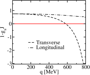
Figure 3: The denominator of the diquark $T$ matrix for the longitudinal and transverse axial vector channel. for parameter set A at $r_{a}=0.44$. Note that there is no longitudinal pole.

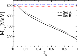
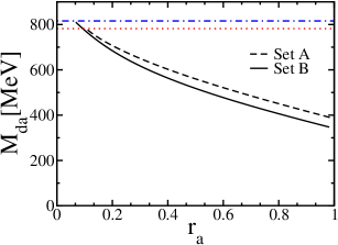
Figure 4: The scalar and axial-vector diquark mass as a function of $r_{s}$ and $r_{a}$, respectively, for both parameter sets. The dotted and the dash-dotted lines denote the quark-quark pseudo-threshold for set A and B, respectively.

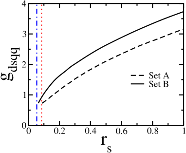
Figure 5: The scalar diquark-quark-quark coupling as a function of $r_{s}$. The dotted and dash-dotted lines indicate the quark-quark pseudo-threshold for set A and B, respectively.

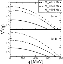
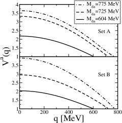
Figure 6: The ratio of the on-shell approximation compared to the exact diquark $T$-matrix for the various scalar and axial diquark masses.

III.1 Diquark Solution

The loop integrations in Eqs. (15,20) are very similar to that appeared in mesonic sector Eq. (9). Therefore, we can employ the same method to evaluate these loop integrations.

We use the parameter sets determined in the mesonic sector shown in table 1. Our numerical computation is valid below the first quark-quark pseudo-threshold. Note that the longitudinal polarizability $J^{L}_{a}(q)$ defined in Eq. (20) does not vanish here. This term will be neglected in our one-pole approximation since it does not produce any poles in the $T$-matrix, and so makes a very small contribution compared to the transverse piece (see Fig. 3). The longitudinal polarizability is not important in the local NJL model as well w ; njln3 . We find that for a wide range of $r_{s}$ and $r_{a}$, for all parameter sets, a bound scalar and axial-vector diquark exist (the results for additional sets can be found in me ). This is in contrast to the normal NJL model where a bound axial-vector diquark exists only for very strong couplings njln3 . The diquark masses for various values of $r_{s}$ and $r_{a}$ are plotted in Fig. 4. As already pointed out, the scalar diquark mass is equal to the pion mass at $r_{s}=1$. It is obvious from Fig. 4 that for $r_{s}=r_{a}$ the axial-vector diquark is heavier than the scalar diquark, and consequently is rather loosely bound. For very small $r_{s}$ and $r_{a}$, one finds no bound state in either diquark channels. In Fig. 5, we show the scalar diquark-quark-quark coupling defined in Eq. (17) with respect to various scalar diquark couplings.

One should note that the nucleon bound state in the diquark-quark picture does not require asymptotic-diquark states since the diquark state is merely an intermediate device which simplifies the three-body problem. Nevertheless, evidence for correlated diquark states in baryons is found in deep-inelastic lepton scatterings and in hyperon weak decays lep2 . At the same time, diquarks appear as bound states in many phenomenological models, and are seen in lattice calculations lat-diq1 ; lat-diq2 . In contrast to our perception of QCD colour confinement, the corresponding spectral functions for these supposedly confined objects in the colour anti-triplet channel are very similar to mesonic ones lat-diq2 .

Next we study the off-shell behaviour of the diquark $T$-matrix. In Fig. 6 we show the discrepancy between the exact $T$-matrix and the on-shell approximation $V^{s,a}(q)$. At the pole we have by definition that $V^{s,a}(q)|_{q^{2}=M^{2}_{s,a}}=1$. We see elsewhere that the off-shell contribution is very important due to the non-locality of our model. We find that the bigger the diquark mass is, the bigger the off-shell contribution. The off-shell behaviour of the scalar and the axial-vector channel for both parameter sets $A$ and $B$ are rather similar.

IV Three-body sector

In order to make the three-body problem tractable, we discard any three-particle irreducible graphs. The relativistic Faddeev equation can be then written as an effective two-body BS equation for a quark and a diquark due to the locality of the form factor in momentum space (see Eq. (3)) and accordingly the separability of the two-body interaction in momentum-space. We adopt the formulation developed by the Tübingen group o1 ; o2 ; o3 to solve the resulting BS equation. In the following we work in momentum space with Euclidean metric. The BS wave function for the octet baryons can be presented in terms of scalar and axialvector diquarks correlations,

$$\psi(p,P)u(P,s)=\left(\begin{array}[]{c}\psi^{5}(p,P)\\ \psi^{\mu}(p,P)\end{array}\right)u(P,s),$$ (23)

where $u(P,s)$ is a basis of positive-energy Dirac spinors of spin $s$ in the rest frame. The parameters $p=(1-\eta)p_{i}-\eta(p_{j}+p_{k})$ and $P=p_{i}+p_{j}+p_{k}$ are the relative and total momenta in the quark-diquark pair, respectively. The Mandelstam parameter $\eta$ describes how the total momentum of the nucleon $P$ is distributed between quark and diquark.

One may alternatively define the vertex function associated with $\psi(p,P)$ by amputating the external quark and diquark propagators (the legs) from the wave function;

$$\phi(p,P)=S^{-1}(p_{q})\tilde{D}^{-1}(p_{d})\left(\begin{array}[]{c}\psi^{5}(p,P)\\ \psi^{\nu}(p,P)\end{array}\right),$$ (24)

with

$$\tilde{D}^{-1}(p_{d})=\left(\begin{array}[]{cc}D^{-1}(p_{d})&0\\ 0&(D^{\mu\nu}(p_{d}))^{-1},\end{array}\right)$$ (25)

where $D(p),D^{\mu\nu}(p)$ and $S(p)$ are Euclidean versions of the diquark and quark propagators which are obtained by the standard transcription rules from the expressions in Minkowski space, Eqs. (16,21) and Eq. (5), respectively. The spectator quark momentum $p_{q}$ and the diquark momentum $p_{d}$ are given by

$$p_{q} = \eta P+p,$$ (26)

$$p_{d} = (1-\eta)P-p,\$$ (27)

with similar expressions for $k_{q,d}$, where we replace $p$ by $k$ on the right-hand side. The Mandelstam parameter $\eta$, parametrises different definitions of the relative momentum within the quark-diquark system. In the ladder approximation, the coupled system of BS equations for octet baryon wave functions and their vertex functions takes the compact form,

Figure 7: The coupled Bethe-Salpeter equation for the vertex function $\phi$.

$$\phi(p,P)=\int\frac{d^{4}k}{(2\pi)^{4}}K^{BS}(p,k;P)\psi(k,P),\\$$ (28)

where $K^{BS}(p,k;P)$ denotes the kernel of the nucleon BS equation representing the exchange quark within the diquark with the spectator quark (see Fig. 7), and in the colour singlet and isospin $\frac{1}{2}$ channel we find (see Ref. njln3 )

$$K^{BS}(p,k;P) = -3\left(\begin{array}[]{cc}\chi^{5}(p_{1},k_{d})S^{T}(q)\bar{\chi}^{5}(p_{2},p_{d})&-\sqrt{3}\chi^{\alpha}(p_{1},k_{d})S^{T}(q)\bar{\chi}^{5}(p_{2},p_{d})\\ -\sqrt{3}\chi^{5}(p_{1},k_{d})S^{T}(q)\bar{\chi}^{\mu}(p_{2},p_{d})&-\chi^{\alpha}(p_{1},k_{d})S^{T}(q)\bar{\chi}^{\mu}(p_{2},p_{d})\end{array}\right),$$ (31)

where $\chi$ and $\chi^{\mu}$ (and their adjoint $\bar{\chi}$ and $\bar{\chi}^{\mu}$) stand for the Dirac structures of the scalar and the axial-vector diquark-quark-quark vertices and can be read off immediately from Eqs. (13, 16) and Eqs. (18, 21), respectively. Therefore we have

$$\chi^{5}(p_{1},k_{d}) = g_{dsqq}(\gamma^{5}C)\sqrt{2V^{s}(k_{d})}f(p_{1}+(1-\sigma)k_{d})f(-p_{1}+\sigma k_{d}),$$

$$\chi^{\mu}(p_{1},k_{d}) = g_{daqq}(\gamma^{\mu}C)\sqrt{2V^{a}(k_{d})}f(p_{1}+(1-\sigma)k_{d})f(-p_{1}+\sigma k_{d}),\$$ (32)

where $\sigma$ is the Mandelstam parameter parameterising different definitions of the relative momentum within the quark-quark system. We have used an improved on-shell approximation for the contribution of diquark $T$-matrix occurring in the Faddeev equations. Instead of the exact diquark $T$-matrices we use the on-shell approximation with a correction of their off-shell contribution through $V^{s,a}(p)$. What is neglected is then the contribution to the $T$-matrix beyond the pseudo-threshold. We will see this approximation is sufficient to obtain a three-body bound state. A similar approximation has been already employed in the normal NJL model in the nucleon sector, see for examples Refs. cut-b ; under2 . One should note that here we do not have continuum states like the normal NJL model. However, there exist many complex poles beyond the pseudo-threshold which may be ignored, provided that they lie well above the energies of interest and the cutoff. For the parameter sets considered here, the next set of poles would result in another pseudo-threshold at energies of $1.3$ GeV and $3$ GeV for sets A and B, respectively. The model is not intended to be reliable at such momenta. On the other hand, as we will see in the next section, in practice, one may escape these poles far enough away by taking advantage of the above Mandelstam parametrization of the momenta.

The relative momentum of quarks in the diquark vertices $\chi$ and $\chi^{\mu}$ are defined as $p_{1}=p+k/2-(1-3\eta)P/2$ and $p_{2}=-k-p/2+(1-3\eta)P/2$, respectively. The momentum $k_{d}$ of the incoming diquark and the momentum $p_{d}$ of the outgoing diquark are defined in Eq. (27) (see Fig. 7). The momentum of the exchanged quark is fixed by momentum conservation at $q=-p-k+(1-2\eta)P$. In the expressions for the momenta we have introduced two independent Mandelstam parameters $\eta,\sigma$, which can take any value in $[0,1]$. Observables should not depend on these parameters if the formulation is Lorentz covariant. This means that for every BS solution $\psi(p,P;\eta_{1},\sigma_{1})$ there exists an equivalent family of solutions. This provides a stringent check on calculations; see the next section for details.

It is interesting to note that the non-locality of the diquark-quark-quark vertices naturally provides a regularisation of the ultraviolet divergence in the diquark-quark loop.

We now constrain the Faddeev amplitude to describe a state of positive energy, positive parity and spin $s=1/2$. The parity condition can be immediately reduced to a condition for the BS wave function:

$$\mathcal{P}\left(\begin{array}[]{c}\psi^{5}(p,P)\\ \psi^{\mu}(p,P)\end{array}\right)=\left(\begin{array}[]{c}\gamma^{4}\psi^{5}(\bar{p},\bar{P})\gamma^{4}\\ \gamma^{4}\Lambda^{\mu\nu}_{\mathcal{P}}\psi^{\nu}(\bar{p},\bar{P})\gamma^{4}\end{array}\right)=\left(\begin{array}[]{c}\psi^{5}(p,P)\\ -\psi^{\mu}(p,P)\end{array}\right),$$ (33)

where we define $\bar{p}=\Lambda_{\mathcal{P}}p$ and $\bar{P}=\Lambda_{\mathcal{P}}P$, with $\Lambda^{\mu\nu}_{\mathcal{P}}=\text{diag}(-1,-1,-1,1)$. In order to ensure the positive energy condition, we project the BS wave function with the positive-energy projector $\Lambda^{+}=(1+\hat{P\kern-6.49994pt/})$, where the hat denotes a unit four vector (in rest frame we have $\hat{P}=P/iM$). Now we expand the BS wave function $\psi(p,P)$ in Dirac space $\Gamma\in\{\textbf{1},\gamma_{5},\gamma^{\mu},\gamma_{5}\gamma^{\mu},\sigma^{\mu\nu}\}$. The above-mentioned conditions reduce the number of independent component from sixteen to eight, two for the scalar diquark channel, $S_{i},(i=1,2)$ and six for the axial-diquark channel, $A_{i},(i=1,...6)$. The most general form of the BS wave function is given by

$$\psi^{5}(p,P) = \left(S_{1}-i\hat{p\kern-4.49997pt/}_{T}S_{2}\right)\Lambda^{+},$$

$$\psi^{\mu}(p,P) = \Big{(}i\hat{P}^{\mu}\hat{p\kern-4.49997pt/}_{T}A_{1}+\hat{P}^{\mu}A_{2}-\hat{p}^{\mu}_{T}\hat{p\kern-4.49997pt/}_{T}A_{3}+i\hat{p}^{\mu}_{T}A_{4}+\left(\hat{p}^{\mu}_{T}\hat{p\kern-4.49997pt/}_{T}-\gamma^{\mu}_{T}\right)A_{5}$$ (34)

$$-(i\gamma^{\mu}_{T}\hat{p\kern-4.49997pt/}_{T}+i\hat{p}^{\mu}_{T})A_{6}\Big{)}\gamma_{5}\Lambda^{+}.\$$

Here we write $\gamma^{\mu}_{T}=\gamma^{\mu}-\hat{P\kern-6.49994pt/}\hat{P}^{\mu}$. The subscript $T$ denotes the component of a four-vector transverse to the nucleon momentum, $p_{T}=p-\hat{P}(p.\hat{P})$. In the same way, one can expand the vertex function $\phi$ in Dirac space, and since the same constraints apply to the vertex function, we obtain an expansion similar to Eq. (34), with new unknown coefficients $\mathbb{S}_{i}$ and $\mathbb{A}_{i}$. The unknown functions $S_{i}(\mathbb{S}_{i})$ and $A_{i}(\mathbb{A}_{i})$ depend on the two scalars which can be built from the nucleon momentum $P$ and relative momentum $p$, $z=\hat{P}.\hat{p}=\cos\omega$ (the cosine of the four-dimensional azimuthal angle of $p^{\mu}$) and $p^{2}$. Of course, they depend on $P^{2}$ as well, but this dependence becomes trivial in the nucleon rest frame.

In the nucleon rest frame, one can rewrite the Faddeev amplitude in terms of tri-spinors each possessing definite orbital angular momentum and spin o1 . It turns out that these tri-spinors can be written as linear combinations of the eight components defined in Eq. (34). Thus from knowledge of $S_{i}$ and $A_{i}$, a full partial wave decomposition can be immediately obtained o1 . Note that the off-shell contribution $V^{s,a}(q)$ is a function of the scalar $q^{2}$. Moreover, the form factor in our model Lagrangian is also scalar, hence the total momentum dependent part of the diquark-quark-quark vertices are scalar functions and carry no orbital angular momentum, i.e. $L^{2}\chi^{5,\mu}(q)=0$. Therefore, the partial wave decomposition obtained in Ref. o1 for pointlike diquarks can be used here. Notice that no such partial wave decomposition can be found for the BS vertex function $\phi^{5,\mu}$ since the axial-vector diquark propagator mixes the space component of the vertex function and time component of the axial-vector diquark.

IV.1 Numerical method for the coupled BS equations

To solve the BS equations we use the algorithm introduced by Oettel et al o4 . The efficiency of this algorithm has already been reported in several publications, see for example Refs. o1 ; o2 ; o3 . We will focus here only on the key ingredients of this method. The momentum dependence of quark mass in our model increases the complexity of the computation significantly. As usual, we work in the rest frame of the nucleon $P=(0,iM_{N})$. In this frame we are free to chose the spatial part of the relative momentum $p$ parallel to the third axis. Thus the momenta $p$ and $k$ are given by

$$p^{\mu} = |p|(0,0,\sqrt{1-z^{2}},z),$$

$$k^{\mu} = |k|(\sin\theta^{\prime}\sin\phi^{\prime}\sqrt{1-z^{\prime 2}},\sin\theta^{\prime}\cos\phi^{\prime}\sqrt{1-z^{\prime 2}},\cos\theta\sqrt{1-z^{\prime 2}},z^{\prime}),\$$ (35)

where we write $z=\cos\omega$ and $z^{\prime}=\cos\omega^{\prime}$. The wave function Eq. (34) consists of $2\times 2$ blocks in Dirac space can be simplified to

$$\psi^{5}(p,P) = \left(\begin{array}[]{cc}S_{1}(p^{2},z)&0\\ \sigma_{3}\sqrt{1-z^{2}}S_{2}(p^{2},z)&0\end{array}\right),\hskip 34.14322pt\psi^{4}(p,P)=\left(\begin{array}[]{cc}\sigma_{3}\sqrt{1-z^{2}}A_{1}(p^{2},z)&0\\ A_{2}(p^{2},z)&0\end{array}\right),$$ (40)

$$\psi^{3}(p,P) = \left(\begin{array}[]{cc}i\sigma_{3}A_{3}(p^{2},z)&0\\ i\sqrt{1-z^{2}}A_{4}(p^{2},z)&0\end{array}\right),\hskip 42.67912pt\psi^{2}(p,P)=\left(\begin{array}[]{cc}i\sigma_{2}A_{5}(p^{2},z)&0\\ -\sigma_{1}\sqrt{1-z^{2}}A_{6}(p^{2},z)&0\end{array}\right),$$ (45)

$$\psi^{1}(p,P) = \left(\begin{array}[]{cc}i\sigma_{1}A_{5}(p^{2},z)&0\\ \sigma_{2}\sqrt{1-z^{2}}A_{6}(p^{2},z)&0\end{array}\right).\$$ (48)

The great advantage of this representation is that the scalar and the axial-vector components are decoupled. Therefore the BS equation decomposes into two sets of coupled equations, two for the scalar diquark channel and six for the axial diquark channel. We expand the vertex (wave) functions in terms of Chebyshev polynomials of the first kind, which are closely related to the expansion into hyperspherical harmonics. This decomposition turns out to be very efficient for such problems o1 ; o2 ; o3 ; o4 . Explicitly,

$$F^{\psi}_{i}(p^{2},z) = \sum^{n_{\text{max}}}_{n=0}i^{n}F^{\psi(n)}_{i}(p^{2})T_{n}(z),$$

$$F^{\phi}_{i}(p^{2},z) = \sum^{m_{\text{max}}}_{m=0}i^{n}F^{\phi(m)}_{i}(p^{2})T_{m}(z),\$$ (49)

where $T_{n}(z)$ is the Chebyshev polynomial of the first kind. We use a generic notation where the functions $F^{\psi}_{i}$(and $F^{\phi}_{i}$) stand for any of the functions $S_{i},~{}A_{i}$ (and $\mathbb{S}_{i},~{}\mathbb{A}_{i}$),

$$S_{1,2}\to F^{\psi}_{1,2},\hskip 56.9055ptA_{1...6}\to F^{\psi}_{3...8},$$

$$\mathbb{S}_{1,2}\to F^{\phi}_{1,2},\hskip 56.9055pt\mathbb{A}_{1...6}\to F^{\phi}_{3...8}.$$ (50)

We truncate the Chebyshev expansions involved in $F^{\psi}_{i}$ and $F^{\phi}_{i}$ at different orders $n_{\text{max}}$ and $m_{\text{max}}$, respectively. We also expand the quark and diquark propagators into Chebyshev polynomials. In this way one can separate the $\hat{P}\cdot\hat{p}$ and $\hat{P}\cdot\hat{k}$ dependence in Eqs. (24,28). Using the orthogonality relation between the Chebyshev polynomials, one can reduce the four dimensional integral equation into a system of coupled one-dimensional equations. Therefore one can rewrite Eqs. (24,28) in the matrix form

$$F^{\psi(n)}_{i}(p^{2}) = \sum_{j=1}^{8}\sum_{m=0}^{m_{\text{max}}}g_{ij}^{nm}(p^{2})F^{\phi(m)}_{j}(p^{2}),$$

$$F^{\phi(m)}_{i}(p^{2}) = \sum_{j=1}^{8}\sum_{n=0}^{n_{\text{max}}}\int^{\infty}_{0}d|k||k|^{3}H_{ij}^{mn}(k^{2},p^{2})F^{\psi(n)}_{j}(k^{2}).\$$ (51)

Here $g_{ij}^{nm}$ and $H_{ij}^{mn}$ are the matrix elements of the propagator and the quark-exchange matrices, respectively. The indices $n,m$ refer to the Chebyshev moments and $i,j$ denote the individual channels. To solve Eq. (51), we first rewrite it in the form of linear eigenvalue problem. Schematically

$$\lambda(P^{2})\varphi=K(P^{2})\varphi,$$ (52)

with the constraint that $\lambda(P^{2})=1$ at $P^{2}=-M^{2}_{N}$. This can be used to determine the nucleon mass $M_{N}$ iteratively.

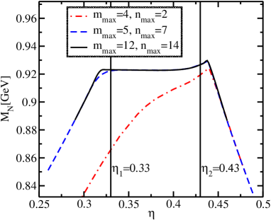
Figure 8: The dependence of the nucleon mass on the Mandelstam parameter $\eta$ for three choices of the cut-off on the Chebyshev expansion. Here we use set B, with $M_{ds}=725$ MeV and $M_{da}=630$ MeV. The vertical lines at $\eta_{1}$ and $\eta_{2}$ denote the position of the singularities defined in Eq. (53).

As already pointed out, the BS solution should be independent of the Mandelstam parameters $\eta,\sigma$. As can be seen in Fig. 8, there is indeed a large plateau for the $\eta$ dependence if we use a high cut-off on the Chebyshev moments. The limitations on the size of this area of stability can be understood by considering where the calculation contains singularities due to quark and diquark poles,

$$\eta \in \left[1-\frac{M_{ds}}{M_{N}},\frac{m^{\text{q}}_{R}}{M_{N}}\right],\hskip 56.9055pt\text{if}\hskip 28.45274ptM_{ds}<M_{da},$$

$$\eta \in \left[1-\frac{M_{da}}{M_{N}},\frac{m^{\text{q}}_{R}}{M_{N}}\right],\hskip 56.9055pt\text{if}\hskip 28.45274ptM_{da}<M_{ds}.$$ (53)

A similar plateau has been found in other applications o1 ; o2 ; o3 . The singularities in the quark-exchange propagator put another constraint on the acceptable range of $\eta$; $\eta>\frac{1}{2}(1-\frac{m^{\text{q}}_{R}}{M_{N}})$. No such constraint exists for $\sigma$, which relates to the relative momentum between two quarks. To simplify the algebra we take $\sigma=1/2$.

In what follows we use a momentum mesh of $60\times 60$ for $p,k$, mapped in a non-linear way to a finite interval. In the non-singular regime of Mandelstam parameter $\eta$ Eq. (53), the Faddeev solution is almost independent of the upper limit on the Chebyshev expansion, and for $m_{\text{max}}=10,n_{\text{max}}=12$, see the Fig. 8, this seems to be satisfied. This limit is somewhat higher than the reported values for simple models o1 ; o2 ; o3 ; o4 .

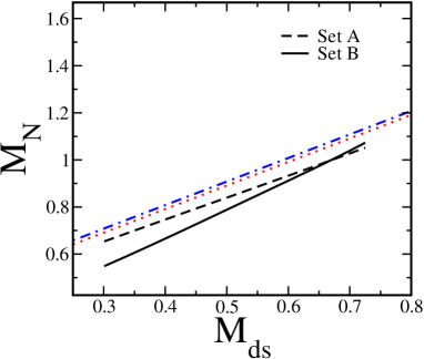
Figure 9: The nucleon mass without inclusion of the axial diquark channel. The dotted lines indicate the diquark-quark threshold. All values are given in GeV.

IV.2 Nucleon Solution

In order to understand the role of the axial diquark in nucleon solution, we first consider the choice $r_{a}=0$. For this case we find that the non-confining set A can not generate a three-body bound state without the inclusion of the off-shell contribution. For the confining set B one also has to enhance the diquark-quark-quark coupling $g_{dsqq}$ by a factor of about $1.73$ over the value defined in Eq. (17) (as we will show, this extra factor is not necessary when the axial-vector diquark is included). The situation is even more severe in the on-shell treatment of the local NJL model, since one needs to include the quark-quark continuum contribution in order to find a three-body bound state when the axial-vector diquark channel is not taken into account njln1 .

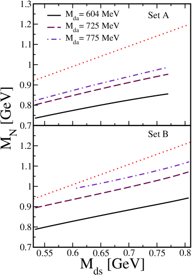
Figure 10: The nucleon mass as a function of the scalar diquark mass for various axial vector diquark masses for both parameter sets. The scalar diquark-quark threshold are shown by the dotted lines.

Figure 11: Range of parameters $(r_{s},r_{a})$ where we find a nucleon mass of $940$ MeV.

As can be seen from Fig. 4 a decrease in $r_{s}$ leads to a larger diquark mass, and an increase in the off-shell contribution to the quark-quark $T$-matrix (see Fig. 6). This off-shell correction is crucial for forming a bound nucleon. If the off-shell contribution $V^{s}(q)$ is omitted, a bound nucleon can not be found.

Table 3: Diquark masses and coupling of diquarks to quarks obtained for $M_{N}=940$ MeV. All masses are given in MeV. $E_{ds}(E_{da})$ denote the binding energy of diquarks in the nucleon, $E^{ds}_{N}(E^{da}_{N})$ denote the binding energy of the nucleon measured from scalar (axial) diquark mass.

	Set A			Set B
	Set A1	Set A2	Set A3	Set B1	Set B2	Set B3
$M_{ds}$	775	748	698	802	705	609
$g_{dsqq}$	0.74	0.83	1.04	0.73	1.31	1.79
$r_{s}$	0.09	0.12	0.17	0.06	0.14	0.24
$E_{ds}$	7	34	84	14	111	207
$E^{ds}_{N}$	226	199	149	270	173	77
$M_{da}$	705	725	775	604	660	725
$g_{daqq}$	1.08	0.98	0.79	1.99	1.67	1.28
$r_{a}$	0.20	0.17	0.11	0.32	0.23	0.15
$E_{da}$	77	57	7	212	156	91
$E^{da}_{N}$	156	176	226	72	123	193
$p_{\bot}^{\text{RMS}}$	194.88	181.51	163.70	283.99	232.86	209.95

The nucleon result is shown in Fig. 9. We also show a fictitious diquark-quark threshold defined as $M_{ds}+m^{\text{q}}_{R}$. The nucleon mass can be seen to depend roughly linearly on the scalar diquark mass. A similar behaviour is also seen in the local NJL model njln2 . Increasing the diquark mass (or decreasing $r_{s}$) increases the nucleon mass, i.e. the scalar diquark channel is attractive. In order to obtain a nucleon mass of $940$ MeV, we need diquark mases of $608$ MeV and $623$ MeV for set A and B, respectively. The corresponding nucleon binding energy measured from the diquark-quark threshold are $56$ MeV and $91$ MeV for set A and B, respectively, compared to the binding of the diquarks (relative to the quark-quark pseudo threshold) of about $174$ and $193$ MeV for set A and B, respectively. Such diquark clustering within the nucleon is also observed in the local NJL model njln2 , and is qualitatively in agreement with an instanton model i-b and lattice simulations lat-bin .

Next we investigate the effect of the axial-vector diquark channel on nucleon solution. We find that the axial-vector diquark channel contributes considerably to the nucleon mass and takes away the need for the artificial enhancement of the coupling strength for set B. In Fig. 10 we show the nucleon mass as a function of the scalar and axial-vector diquark mass. As in the scalar diquark channel, we define the axial-vector diquark-quark threshold as $M_{da}+m^{\text{q}}_{R}$. We see that as one increases the axial-vector diquark (and scalar diquark) masses, the quark-quark interaction is weakened and consequently the nucleon mass increases. Therefore the contribution of the axial-vector channel to the nucleon mass is also attractive.

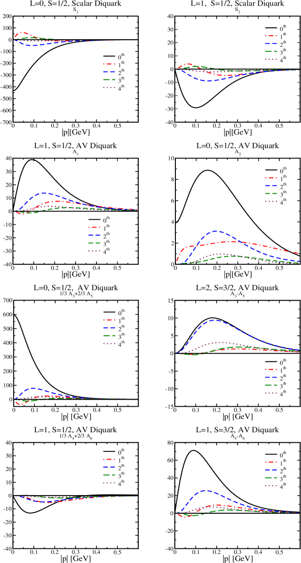
Figure 12: Chebyshev moments (labelled by $n$) of the scalar and axial-vector (AV) diquark amplitudes of the nucleon BS wave function given by Set A1.

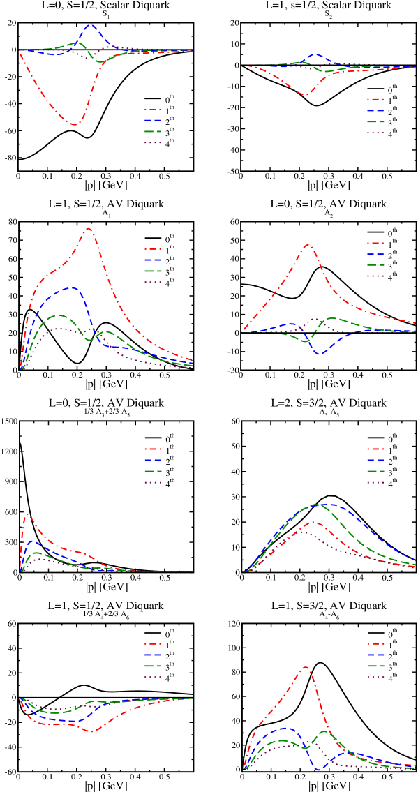
Figure 13: Chebyshev moments (labelled by the order $n$) of scalar and axial-vector (AV) diquark amplitudes for the nucleon BS wave function obtained for parameter set B1.

In Fig. 11 we plot the parameter space of the interaction Lagrangian with variable $r_{s}$ and $r_{a}$ which leads to the nucleon mass $M_{N}=940$ MeV. The trend of this plot for the non-confining set A is very similar to the one obtained in the local NJL model njln3 .

If the scalar diquark interaction $r_{s}$ is less than $0.14$, we need the axial-vector interaction to be stronger than the scalar diquark channel $r_{a}>r_{s}$ in order to get the experimental value of nucleon mass. For set B, as we approach $r_{a}=0$, the curve bends upward, reflecting the fact that we have no bound state with only the scalar diquark channel.

In Fig. 11 we see for the confining set B that the interaction is again shared between the scalar and the axial-vector diquark and for small $r_{s}<0.19$ one needs a dominant axial-vector diquark channel $r_{a}>r_{s}$. It is obvious that the axial-vector diquark channel is much more important in the confining than the non-confining phase of model.

Figure 14: Diagram corresponding to the definition of density Eq. (54).

In order to study the implications of the quark confinement for the description of the nucleon, we compare in Table 3 three representative cases for both the non-confining and confining parameter sets, which all give a nucleon mass of about $940$ MeV. The first three columns contain results for set $A$, and the last three columns for the confining set $B$.

Given the definition of diquark-quark thresholds, in the presence of both scalar and axial-vector diquark channels, the diquarks in the nucleon can be found much more loosely bound, although one obtains a very strongly bound nucleon solution near its experimental value, see table 3. Next we study the nucleon BS wave function for the various sets given in Table 3. The nucleon wave and vertex function are not physical observables, but rather they suggest how observables in this model will behave. In Figs. 12, 13 we show the leading Chebyshev moments of the scalar functions of the nucleon BS wave function for various sets (A1 and B1). They describe the strengths of the quark-diquark partial waves with $S$ as a total quark-diquark spin and $L$ as a total orbital angular momentum. They are normalised to $F_{1}^{\phi(0)}(p_{1})=1$, where $p_{1}$ is the first point of the momentum mesh. Very similar plots are found for the other sets of parameters given in table 3. It is seen that the contribution of higher moments are considerably smaller than lower ones, indicating a rapid convergence of the expansion in terms of Chebyshev polynomials. In the confining case, Fig. 13, there is a clear interference which is not present in the non-confining one, Fig. 12. Therefore in the confining case, all wave function amplitudes are shifted to higher relative four-momenta between the diquark and quark.

In order to understand the effect of this interference, we construct a density function for the various channels in the nucleon rest frame. This density is defined as

$$\rho(p_{\bot},P)=\int dp_{4}\psi^{{\dagger}}(p_{\bot},p_{4},P)\tilde{D}^{-1}(p_{d})\psi(p_{\bot},p_{4},P),$$ (54)

where $p_{\bot}$ stands for the space component of the relative momentum $p$, and $\tilde{D}^{-1}(p_{d})$ is defined in Eq. (25). This definition corresponds to a very naive diagram describing the quark density within the nucleon, see Fig. 14. In the above definition of the density function, we have integrated over the time component of the relative momentum. In this way the density function becomes very similar to its counterpart in Minkowski space. Although the above definition of density is not unique, it does provide a useful measure of the spatial extent of the wave function. Similar calculations have been done for the quark condensate in Ref. njln4-is . The results are plotted in Figs. 15 and 16.

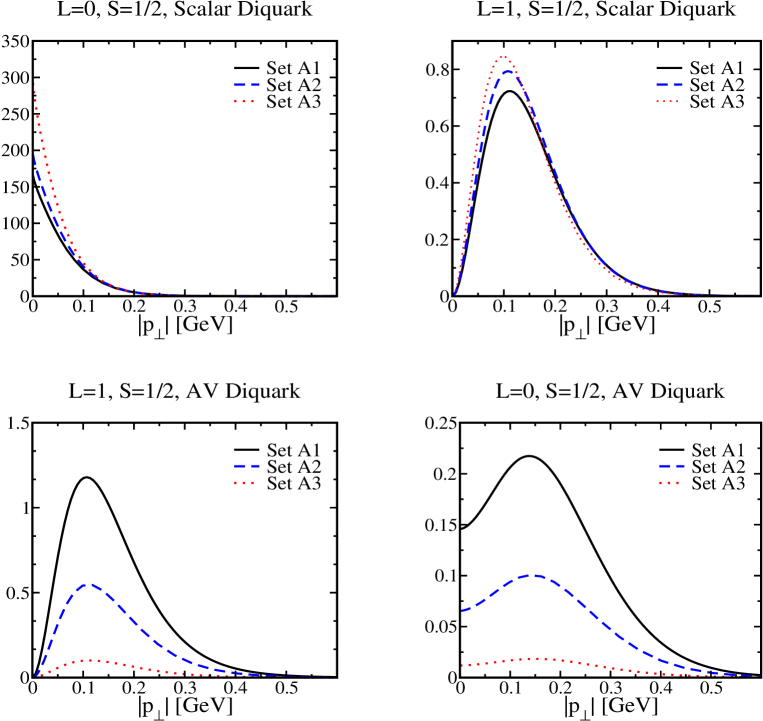
Figure 15: Shows the nucleon density ($M=940$ MeV, Set $A$) with respect to relative momentum between diquark and quark for different set of $A1,A2$ and $A3$.

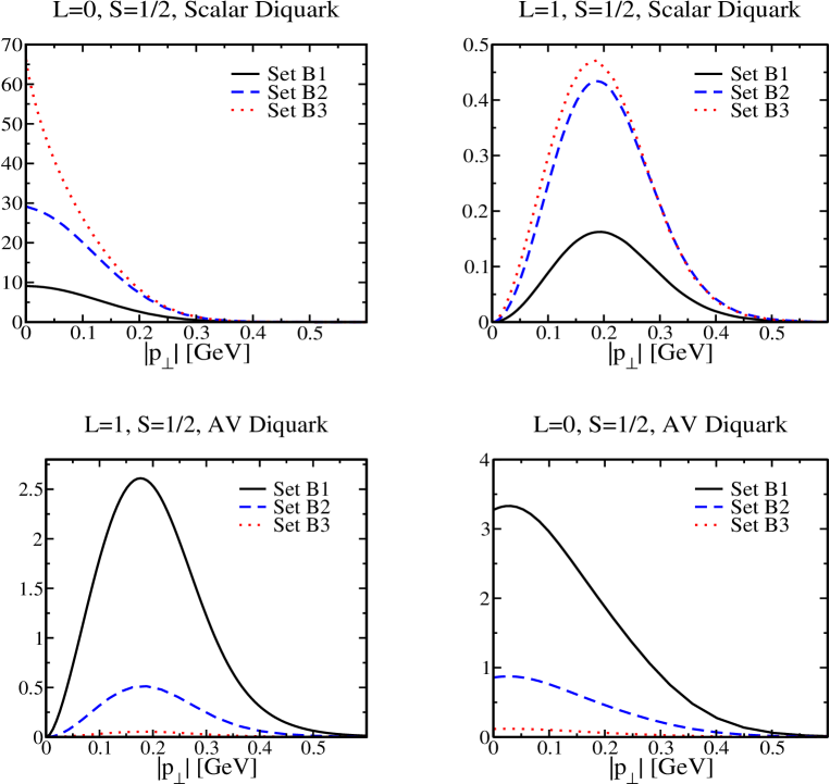
Figure 16: Shows the nucleon density ($M=940$ MeV, Set $B$) with respect to relative momentum between diquark and quark for different set of $B1,B2$ and $B3$.

It is noticeable that in all cases, the $s$-wave in scalar diquark channel is the dominant contribution to the ground state. The relative importance of the scalar and the axial diquark amplitude in the nucleon changes with the strength of the diquark-quark couplings $g_{dsqq}(g_{daqq})$ and accordingly with $r_{s}(r_{a})$. There are indications that in the confining sets, the nucleon density extends to higher relative momentum between the diquark and the quark. These imply a more compact nucleon in the confining cases. In order to find a quantitative estimate of the confinement effect in our model, we calculate $p_{\bot}^{\text{RMS}}=(\langle p^{2}_{\bot}\rangle-\langle p_{\bot}\rangle^{2})^{1/2}$; the results can be found in table 3.

We also see in the both confining and non-confining cases a decrease in $p_{\bot}^{\text{RMS}}$ with weakening axial-vector diquark interaction (and consequently increasing the scalar diquark interaction strength). This can be associated with the important role of the axial-vector diquarks. If we compare $p_{\bot}^{\text{RMS}}$ for the two sets $A2$ and $B2$, which have very similar interaction parameters $r_{s}(r_{a})$, an increase about $25\%$ is found.

V Summary and Outlook

In this work we have investigated the two- and three-quark problems in a non-local NJL model. We have truncated the diquark sector to the scalar and the axial-vector channels. We have solved the relativistic Faddeev equation for this model and have studied the behaviour of the nucleon solutions with respect to various scalar and the axial-vector interactions. We have studied the dependence of the baryon masses and waves on the interaction parameters $r_{s}$ and $r_{a}$ (and on the scalar and the axial-vector diquark mases), which can describe the pion and the nucleon simultaneously. In order to put more restrictions on these parameters, one would need to calculate the $\Delta$ mass as well.

Although the model is quark confining, it is not diquark confining (at least in the rainbow-ladder approximation). A bound diquark can be found in both scalar and the axial-vector channel for a wide range of couplings. We have found that the off-shell contribution to the diquark $T$-matrix is crucial for the calculation of the nucleon: without it the attraction in the diquark channels is too weak to form a three-body bound state. We have also found that both the scalar and the axial-vector contribute attractively to the nucleon mass. The role of axial-vector channel is much more important in the confining phase of model. The nucleon in this model is strongly bound even though the diquarks are rather loosely bound. The confining aspects of the model are more obvious in three-body, rather than the two-body sector. We decomposed the nucleon BS wave function in the nucleon rest frame in terms of spin and orbital angular momentum eigenstates and constructed the quark density function in the various channels. It was revealed that $s$-wave in scalar diquark channel is the dominant contribution to the ground state. By investigating the nucleon wave function we found that quark confinement leads to a more compact nucleon. The size of nucleon is reduced by about $25\%$ in the confining cases.

For both confining and non-confining cases, an increase in the scalar diquark channel interaction $r_{s}$ leads to a lower nucleon mass, see Fig. 10. However, the mass of the $\Delta$ should be independent of $r_{s}$ since it does not contain scalar diquarks njln3 ; o1 ; i-b . In the standard NJL model the difference between the nucleon and $\Delta$ masses is strongly dependent on the scalar diquark interaction njln3 . In the current model where the axial-vector diquark makes a larger contribution to the nucleon mass, a detailed calculation of the $\Delta$ is needed to understand the mechanism behind the $\Delta$-$N$ mass difference. Note also that neglecting $\pi N$-loops may lead to a quantitative overestimate of the axial-vector diquark role in the nucleon pion-n .

In order to understand the implications of this model in baryonic sector fully one should investigate other properties of the nucleons such as the charge radii, magnetic moments and axial coupling. On the other hand, the role of quark confinement in this model may be better clarified by investigating quark and nuclear matter in this model. Such problems can also be studied within the same Faddeev approach w ; njl-av .

References

- (1) For a review see: S. P. Klevansky, Rev. Mod. Phys. 64, 649 (1992).
- (2) M. Oertel, M. Buballa and J. Wambach, Phys. Lett. B477, 77 (2000) [hep-ph/9908475]; Nucl. Phys. A676, 247 (2000)[hep-ph/0001239]; G. Ripka, Nucl. Phys. A683 463, 486 (2001) [hep-ph/0003201].
- (3) G. Hellstern and C. Weiss, Phys. Lett. B351, 64 (1995) [hep-ph/9502217].
- (4) For examples see: M. Buballa, hep-ph/0402234 and references therein.
- (5) S. Pepin, M. C. Birse, J. A. McGovern and N. R. Walet, Phys. Rev. C61, 055209 (2000) [hep-ph/9912475].
- (6) L. von Smekal, P. A. Amundsen and R. Alkofer, Nucl. Phys. A529, 633 (1991).
- (7) J. M. Cornwall, Phys. Rev. D22, 1452 (1980); M. Stingl, Phys. Rev. D34, 3863 (1986); D36, 651 (1987); V. Sh. Gogoghia and B. A. Magradze, Phys. lett. B217, 162 (1989).
- (8) C. D. Roberts and A. G. Williams, Prog. Part. Nucl. Phys. 33, 477 (1994) [hep-ph/9403224]; C. D. Roberts and S. M. Schmidt, Prog. Part. Nucl. Phys. 45, S1 (2000) [nucl-th/0005064].
- (9) K. Langfeld and M. Rho, Nucl. Phys. A596, 451 (1996) [hep-ph/9506265]; D. Ebert, T. Feldmann and H. Reinhardt, Phys. Lett. B388, 154 (1996) [hep-ph/9608223].
- (10) D. Diakonov, V. Yu. Petrov, Sov. Phys. JETP 62, 204 (1985); Nucl. Phys. B245, 259 (1984); D. Diakonov, V. Yu. Petrov, P. V. Pobylitsa, Nucl. Phys. B306, 809 (1988); I. V. Anikin, A. E. Dorokhov and L. Tomio, Phys. Part. Nucl. 31, 509 (2000) [hep-ph/9909368].
- (11) R. D. Bowler and M. C. Birse, Nucl. Phys. A582, 655 (1995) [hep-ph/9407336]; R. S. Plant and M. C. Birse, Nucl. Phys. A628, 607 (1998) [hep-ph/9705372].
- (12) R. S. Plant and M. C. Birse, Nucl. Phys. A703, 717 (2002) [hep-ph/0007340].
- (13) A. Scarpettini, D. G. Dumm and N. N. Scoccola, Phys. Rev. D69, 114018 (2004) [ hep-ph/0311030].
- (14) D. Atkinson and D. W. E. Blatt, Nucl. Phys. B151, 342 (1979).
- (15) P. Maris and H. A. Holties, Int. J. Mod. Phys. A7, 5369 (1992); S. J. Stainsby and R. T. Cahill, Int. J. Mod. Phys. A7, 7541 (1992); P. Maris, Phys. Rev. D50, 4189 (1994).
- (16) P. Maris, Phys. Rev. D52, 6087 (1995) [hep-ph/9508323].
- (17) J. Skullerud, D. B. Leinweber and A. G. Williams, Phys. Rev. D64, 074508 (2001) [hep-lat/0102013].
- (18) B. Holdom, J. Terning and K. Verbeek, Phys. Lett. B232, 351 (1989); J. W. Bos, J. H. Koch and H. W. L. Naus, Phys. Rev. C44, 485 (1991); R. D. Ball and G. Ripka, in Many Body Physics (Coimbra 1993), edited by C. Fiolhais, M. Fiolhais, C. Sousa and J. N. Urbano (World Scientific, Singapore, 1993).
- (19) T. Schäfer and E. V. Shuryak, Rev. Mod. Phys. 70, 323 (1998) [hep-ph/9610451]; D. Diakonov, Prog. Part. Nucl. Phys. 36, 1 (1996).
- (20) H. Ito, W. W. Buck and F. Gross, Phys. Lett. B248, 28 (1990); H. Ito, W. Buck and F. Gross, Phys. Rev. C43, 2483 (1991).
- (21) G. V. Efimov and S. N. Nedelko, Phys. Rev. D51, 176 (1995); Y. V. Burdanov, G. V. Efimov, S. N. Nedelko and S. A. Solunin, Phys. Rev. D54, 4483 (1996) [hep-ph/9601344].
- (22) I. General, D. G. Dumm and N. N. Scoccola, Phys. Lett. B506, 267 (2001) [hep-ph/0010034]; D. G. Dumm and N. N. Scoccola, Phys. Rev. D65, 074021 (2002) [hep-ph/0107251].
- (23) W. Broniowski, B. Golli and G. Ripka, Nucl. Phys. A703, 667 (2002) [hep-ph/0107139]; B. Golli, W. Broniowski and G. Ripka, Phys. Lett. B437, 24 (1998) [hep-ph/9807261].
- (24) A. Buck, R. Alkofer and H. Reinhardt, Phys. Lett. B286, 29 (1992).
- (25) S. Huang and J. Tjon, Phys. Rev. C49, 1702 (1994) [hep-ph/9308362].
- (26) N. Ishii, W. Bentz, K. Yazaki, Nucl. Phys. A587,617 (1995).
- (27) H. Asami, N. Ishii, W. Bentz and K. Yazaki, Phys. Rev. C51, 3388 (1995).
- (28) C. Hanhart and S. Krewald, Phys. Lett. B344, 55 (1995).
- (29) M. Oettel, G. Hellstern, R. Alkofer and H. Reinhardt, Phys. Rev. C58, 2459, (1998) [nucl-th/9805054].
- (30) G. Hellstern, R. Alkofer, M. Oettel and H. Reinhardt, Nucl. Phys. A627, 679 (1997) [ hep-ph/9705267]; M. Oettel, R. Alkofer and L. von Smekal, Eur. Phys. J. A8, 553 (2000) [nucl-th/0006082].
- (31) S. Ahlig, R. Alkofer, C.S. Fischer, M. Oettel, H. Reinhardt and H. Weigel, Phys. Rev. D64, 014004 (2001) [ hep-ph/0012282].
- (32) M. Oettel, L. Von Smekal, R. Alkofer, Comput. Phys. Commun. 144, 63 (2002) [hep-ph/0109285].
- (33) R. E. Cutkosky, P. V. Landshoff, D. I. Olive and J. C. Polkinghorne, Nucl. Phys. B12, 281 (1969).
- (34) M. S. Bhagwat, M. A. Pichowsky and P.C. Tandy, Phys. Rev. D67, 054019 (2003).
- (35) H.G. Dosch and S. Narison, Phys. Lett.B417,173 (1998) [hep-ph/9709215].
- (36) L. Giusti, F. Rapuano, M. Talevi and A. Vladikas, Nucl. Phys. B538, 249 (1999) [hep-lat/9807014].
- (37) C. Weiss, Phys. Lett. B333, 7 (1994) [hep-ph/9404301].
- (38) A. H. Rezaeian, N. R. Walet and M. C. Birse, hep-ph/0310013.
- (39) M. Anselmino, E. Predazzi, S. Ekelin, S. Fredriksson and D. B. Lichtenberg, Rev. Mod. Phys. 65, 1199 (1993) and references therein.
- (40) M. Hess, F. Karsch, E. Laermann and I. Wetzorke, Phys. Rev. D58, 111502 (1998) [hep-lat/9804023].
- (41) I. Wetzorke and F. Karsch, hep-lat/0008008.
- (42) W. Bentz and A. W. Thomas, Nucl. Phys. A696, 138 (2001) [nucl-th/0105022].
- (43) T. Schäfer, E. V. Shuryak and J. J. M. Verbaarschot, Nucl. Phys. B412, 143 (1994) [hep-ph/9406210].
- (44) M. C. Chu, J.M. Grandy, S. Huang and J. W. Negele, Phys. Rev. D49, 6039 (1994).
- (45) N. Ishii, Phys. Lett. B431, 1 (1998); M. B. Hecht, M. Oettel, C. D. Roberts, S. M. Schmidt, P. C. Tandy and A. W. Thomas, Phys. Rev. C65, 055204 (2002) [nucl-th/0201084].
- (46) H. Mineo, W. Bentz, N. Ishii and K. Yazaki, Nucl. Phys. A703, 785 (2002) [nucl-th/0201082].