CLNS 04/1870

LMU 03/04

August 2004

Constraining the Unitarity Triangle
with $B\to V\gamma$

Stefan W. Bosch^a and Gerhard Buchalla^b
aInstitute for High-Energy Phenomenology
Newman Laboratory for Elementary-Particle Physics, Cornell University
Ithaca, NY 14853, U.S.A.
^b Ludwig-Maximilians-Universität München, Department für Physik
Theresienstraße 37, D-80333 Munich, Germany

We discuss the exclusive radiative decays $B\to K^{*}\gamma$, $B\to\rho\gamma$, and $B\to\omega\gamma$ in QCD factorization within the Standard Model. The analysis is based on the heavy-quark limit of QCD. Our results for these decays are complete to next-to-leading order in QCD and to leading order in the heavy-quark limit. Special emphasis is placed on constraining the CKM-unitarity triangle from these observables. We propose a theoretically clean method to determine CKM parameters from the ratio of the $B\to\rho l\nu$ decay spectrum to the branching fraction of $B\to\rho\gamma$. The method is based on the cancellation of soft hadronic form factors in the large energy limit, which occurs in a suitable region of phase space. The ratio of the $B\to\rho\gamma$ and $B\to K^{*}\gamma$ branching fractions determines the side $R_{t}$ of the standard unitarity triangle with reduced hadronic uncertainties. The recent Babar bound on $B(B^{0}\to\rho^{0}\gamma)$ implies $R_{t}<0.81\,(\xi/1.3)$, with the limiting uncertainty coming only from the SU(3) breaking form factor ratio $\xi$. This constraint is already getting competitive with the constraint from $B_{s}$-$\bar{B}_{s}$ mixing. Phenomenological implications from isospin-breaking effects are briefly discussed.

1 Introduction

The radiative transition $b\to s\gamma$ is one of the most important processes for the study of flavour physics. As a flavour-changing neutral current interaction it is a genuine quantum effect within the Standard Model (SM) and has a high sensitivity to new dynamics at short-distance scales. The cleanest way to probe $b\to s\gamma$ is the measurement of the inclusive decay $B\to X_{s}\gamma$, where the impact of strong interactions is well under control (see [1] for a recent review). For exclusive channels such as $B\to K^{*}\gamma$, which depend on hadronic quantities describing the hadronization of the final state quarks into a single $K^{*}$, a theoretical treatment is more difficult. At present, the decay $B\to X_{s}\gamma$ already yields strong tests of the SM and valuable constraints on its possible extensions.

In contrast, not much is currently known experimentally about $b\to d\gamma$ transitions, the Cabibbo-suppressed counterparts of $b\to s\gamma$. They depend on the less well determined weak mixing parameter $V_{td}$, rather than $V_{ts}$, and could be differently affected by new physics. For these reasons a measurement of $b\to d\gamma$ will be very important. However, the inclusive measurement of $B\to X_{d}\gamma$, theoretically prefered, appears almost impossible because of the dominating background from $B\to X_{s}\gamma$. Therefore, exclusive channels such as $B\to\rho\gamma$ and $B\to\omega\gamma$ become the only way to access $b\to d\gamma$ transitions in the foreseeable future.

The CP-averaged branching ratios of exclusive radiative channels are measured to be [2]

$$B(B^{0}\to K^{*0}\gamma) = (4.01\pm 0.20)\cdot 10^{-5}$$ (1)

$$B(B^{+}\to K^{*+}\gamma) = (4.03\pm 0.26)\cdot 10^{-5}$$ (2)

and bounded with 90% confidence level by Babar as [3]

$$B(B^{0}\to\omega^{0}\gamma) < 1.0\cdot 10^{-6}$$ (3)

$$B(B^{0}\to\rho^{0}\gamma) < 0.4\cdot 10^{-6}$$ (4)

$$B(B^{+}\to\rho^{+}\gamma) < 1.8\cdot 10^{-6}$$ (5)

The corresponding results from Belle read [4]

$$B(B^{0}\to\omega^{0}\gamma) < 0.8\cdot 10^{-6}$$ (6)

$$B(B^{0}\to\rho^{0}\gamma) < 0.8\cdot 10^{-6}$$ (7)

$$B(B^{+}\to\rho^{+}\gamma) < 2.2\cdot 10^{-6}$$ (8)

Even though a theoretical treatment of the exclusive decays $B\to\rho\gamma$, $B\to\omega\gamma$, and $B\to K^{*}\gamma$ is more challenging than of the inclusive modes, there are circumstances that help us to make this task tractable and that will eventually yield useful phenomenological results. First, recent studies of exclusive hadronic modes in the heavy-quark limit have led to a better understanding of the strong dynamics of these decays [5, 6, 7] by establishing factorization formulas in QCD. For the decays $B\to V\gamma$ [6, 7] this approach resulted in particular in a calculation of light-quark loop amplitudes that before constituted an uncontrollable source of uncertainty. In addition it became possible to extend the computation of $B\to V\gamma$ amplitudes systematically to next-to-leading order (NLO) in QCD [6, 7, 8], improving on previous analyses [9, 10]. Second, the impact of hadronic form factors, which dominates theoretical uncertainties, can be reduced by taking the ratio $B(B\to\rho\gamma)/B(B\to K^{*}\gamma)$. The ratio of the corresponding form factors is equal to unity in the limit of $SU(3)$-flavour symmetry and the hadronic uncertainty is reduced to the effect of $SU(3)$ breaking, which still needs to be estimated. Furthermore, the ratio of the $B\to\rho\gamma$ and $B\to K^{*}\gamma$ branching fractions is, at leading order in $\alpha_{s}$, directly proportional to the side $R_{t}$ in the standard unitarity triangle (UT), where

$$R_{t}\equiv\sqrt{(1-\bar{\rho})^{2}+\bar{\eta}^{2}}=\frac{1}{\lambda}\left|\frac{V_{td}}{V_{ts}}\right|$$ (9)

Here $\lambda$, $\bar{\rho}$, and $\bar{\eta}$ are Wolfenstein parameters. Having the complete NLO result for the decay amplitudes in $B\to V\gamma$ at hand, we can calculate $\alpha_{s}$ corrections to their relation with $R_{t}$ and evaluate the implications in the ($\bar{\rho},\bar{\eta})$ plane [11, 12, 13].

Another possibility to reduce hadronic uncertainties consists in taking the ratio of $B\to\rho l\nu$ and $B\to\rho\gamma$ branching fractions. Using relations between the $B\to\rho$ form factors in the large energy linit, it can be shown that this ratio is free of long-distance QCD effects in a certain region of $B\to\rho l\nu$ phase space. The form factors cancel in this situation, up to calculable ${\cal O}(\alpha_{s})$ corrections, which leads to a model-independent relationship of $B\to\rho l\nu$ and $B\to\rho\gamma$ observables to the CKM quantity

$$\left|\frac{V_{ud}V_{ub}}{V_{td}V_{tb}}\right|^{2}=\frac{\bar{\rho}^{2}+\bar{\eta}^{2}}{(1-\bar{\rho})^{2}+\bar{\eta}^{2}}$$ (10)

It is the purpose of this paper to investigate how $B\to V\gamma$ decays can be used to constrain the parameters of the unitarity triangle. Such constraints simultaneously provide a test for new physics. The various sources of uncertainty will be discussed in detail in order to quantify the potential of these important decays. In section 2 we recall the analysis of $B\to V\gamma$ decays at next-to-leading order within the framework of factorization in the heavy-quark limit. The extraction of CKM parameters based on the ratios $B(B\to\rho\gamma)/B(B\to K^{*}\gamma)$ is the subject of section 3. In section 4 we discuss how theoretically clean information on CKM quantities can be obtained from combining a measurement of $B(B\to\rho^{0}\gamma)$ with a Dalitz-plot analysis of $B\to\rho l\nu$ decays. Section 5 contains an update on observables of isospin breaking in $B\to V\gamma$ and section 6 is devoted to a discussion of the decay mode $B\to\omega\gamma$. We present our conclusions in section 7.

2 $B\to V\gamma$ at NLO in QCD

Let us briefly summarize the basic formulas relevant for the analysis of $B\to V\gamma$ at next-to-leading order in QCD. For more details we refer the reader to [6, 14]. The effective weak Hamiltonian for $b\to s\gamma$ transitions is

$${\cal H}_{eff}=\frac{G_{F}}{\sqrt{2}}\sum_{p=u,c}\lambda_{p}^{(s)}\bigg{(}\sum_{i=1}^{2}C_{i}Q^{p}_{i}+\sum_{j=3}^{8}C_{j}Q_{j}\bigg{)}$$ (11)

where

$$\lambda_{p}^{(s)}=V^{*}_{ps}V_{pb}$$ (12)

The relevant operators are the current-current operators $Q^{p}_{1,2}$, the QCD-penguin operators $Q_{3\ldots 6}$, and the electro- and chromomagnetic penguin operators $Q_{7,8}$. The most important contributions come from $Q^{p}_{1,2}$ and $Q_{7,8}$, which read

$$Q^{p}_{1}=(\bar{s}p)_{V-A}(\bar{p}b)_{V-A}\qquad Q^{p}_{2}=(\bar{s}_{i}p_{j})_{V-A}(\bar{p}_{j}b_{i})_{V-A}$$ (13)

$$Q_{7}=\frac{e}{8\pi^{2}}m_{b}\,\bar{s}_{i}\sigma^{\mu\nu}(1+\gamma_{5})b_{i}\,F_{\mu\nu}\qquad Q_{8}=\frac{g}{8\pi^{2}}m_{b}\,\bar{s}_{i}\sigma^{\mu\nu}(1+\gamma_{5})T^{a}_{ij}b_{j}\,G^{a}_{\mu\nu}$$ (14)

The impact of penguin operators $Q_{3},\ldots Q_{6}$ is very small for most applications, but will be included in the numerical results presented below. The effective Hamiltonian for $b\to d\gamma$ is obtained from (11)–(14) by the replacement $s\to d$.

To evaluate the hadronic matrix elements of these operators we employ the heavy-quark limit $m_{b}\gg\Lambda_{\mathrm{QCD}}$ to get the factorization formula [6, 7]

$$\langle V\gamma(\epsilon)|Q_{i}|\bar{B}\rangle=\Big{[}F_{V}T^{I}_{i}+\!\int^{1}_{0}\!\!d\xi\,dv\,T^{II}_{i}(\xi,v)\Phi_{B}(\xi)\Phi_{V}(v)\Big{]}\!\cdot\epsilon$$ (15)

where $\epsilon$ is the photon polarization 4-vector. Here $F_{V}$ is a $B\to V$ transition form factor, and $\Phi_{B}$, $\Phi_{V}$ are leading-twist light-cone distribution amplitudes of the $B$ meson and the vector meson $V$, respectively. These quantities are universal, nonperturbative objects. They describe the long-distance dynamics of the matrix elements, which is factorized from the perturbative, short-distance interactions expressed in the hard-scattering kernels $T^{I}_{i}$ and $T^{II}_{i}$. The QCD factorization formula (15) holds up to corrections of relative order $\Lambda_{QCD}/m_{b}$.

To leading order in QCD and leading power in the heavy-quark limit, $Q_{7}$ gives the only contribution to the $B\to V\gamma$ amplitude. Its matrix element is simply expressed in terms of the standard form factor, $T^{I}_{7}$ is a purely kinematical function, and the spectator term $T^{II}_{7}$ is absent. At ${\cal O}(\alpha_{s})$ the operators $Q_{1\ldots 6}$ and $Q_{8}$ start contributing and the factorization formula becomes nontrivial.

The relevant diagrams for the NLO hard-vertex corrections $T_{i}^{I}$ have been computed in [15, 16] to get the virtual corrections to the matrix elements for the inclusive $b\to s\gamma$ mode at next-to-leading order. For the exclusive modes the same corrections enter the perturbative type I hard-scattering kernels. The non-vanishing contributions to $T^{II}_{i}$, where the spectator participates in the hard scattering, are shown in Fig. 1.

Figure 1: ${\cal O}(\alpha_{s})$ contribution at leading power to the hard-scattering kernels $T^{II}_{i}$ from four-quark operators $Q_{i}$ (left) and from $Q_{8}$. The crosses indicate the places where the emitted photon can be attached.

We can express both the type I and type II contributions to the matrix elements $\langle Q_{i}\rangle$ in terms of the matrix element $\langle Q_{7}\rangle$, an explicit factor of $\alpha_{s}$, and hard-scattering functions $G_{i}$ and $H_{i}$, which are given in [6, 14].

Weak annihilation contributions are suppressed by one power of $\Lambda_{\mathrm{QCD}}/m_{b}$ but nevertheless calculable in QCD factorization, because in the heavy-quark limit the colour-transparency argument applies to the emitted, highly energetic vector meson. Despite their suppression in $\Lambda_{\mathrm{QCD}}/m_{b}$, they can be enhanced by large Wilson coefficients $C_{1,2}$ and thus still give important corrections. This situation is relevant for $B\to\rho\gamma$. Weak annihilation is sensitive to the charge of the decaying $B$ meson and thus leads to isospin-breaking differences between $B^{+}\to\rho^{+}\gamma$ and $B^{0}\to\rho^{0}\gamma$. The corresponding mechanism is CKM suppressed in the case of $B\to K^{*}\gamma$, where penguin operators give the dominant effect for isospin breaking.

The total $\bar{B}\to V\gamma$ amplitude then can be written as

$$A(\bar{B}\to V\gamma)=\frac{G_{F}}{\sqrt{2}}\left[\lambda_{u}a^{u}_{7}+\lambda_{c}a^{c}_{7}\right]\langle V\gamma|Q_{7}|\bar{B}\rangle$$ (16)

where the factorization coefficients $a_{7}^{p}(V\gamma)$ consist of the Wilson coefficient $C_{7}$, the contributions from the type-I and type-II hard-scattering, and annihilation corrections. One finds a sizeable enhancement of the leading order value, dominated by the $T^{I}$-type correction. The net enhancement of $a_{7}$ at NLO leads to a corresponding enhancement of the branching ratios, for fixed value of the form factor. This is illustrated in Fig. 2,

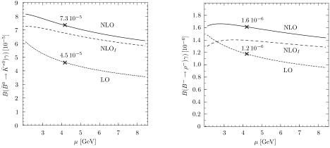
Figure 2: Dependence of the branching fractions $B(\bar{B}^{0}\to\bar{K}^{*0}\gamma)$ and $B(B^{-}\to\rho^{-}\gamma)$ on the renormalization scale $\mu$. The dotted line shows the LO, the dash-dotted line the NLO result including type-I corrections only and the solid line shows the complete NLO result.

where we show the residual scale dependence for $B(\bar{B}\to\bar{K}^{*0}\gamma)$ and $B(B^{-}\to\rho^{-}\gamma)$ at leading and next-to-leading order. As shown already in [6, 14], our central values for the $B\to K^{*}\gamma$ branching ratios are higher than the experimental measurements (1), (2). The dominant theoretical uncertainty comes from the $B\to V\gamma$ form factors. We used the light-cone sum rule (LCSR) results $F_{K^{*}}=0.38\pm 0.06$ and $F_{\rho}=0.29\pm 0.04$ from [17]. A recent preliminary lattice QCD determination, $F_{K^{*}}=0.25\pm 0.05\pm 0.02$ [18], would give a better agreement with the experimental central values. Further studies of heavy-to-light form factors will also benefit from developments based on factorization and soft-collinear effective theory (for recent discussions see [19, 20, 21, 22]).

Using the experimental results for the exclusive $B^{0}\to K^{*0}\gamma$ and inclusive $B\to X_{s}\gamma$ branching ratios together with their theory predictions, we could extract a value of the $B\to K^{*}$ form factor that is essentially independent of CKM factors and potential new physics effects. The most recent measurement of the inclusive branching ratio comes from the Belle collaboration, which reports [23]

$$B(B\to X_{s}\gamma)^{\rm exp}_{E_{\gamma>1.8\,\rm{GeV}}}=(3.59\pm 0.47)\cdot 10^{-4}$$ (17)

in the photon energy range 1.8 GeV $\leq E_{\gamma}\leq$ 2.8 GeV. The theory predicition from a complete NLO QCD calculation is [16]

$$B(B\to X_{s}\gamma)^{\rm th}_{E_{\gamma>1.6\,\rm{GeV}}}=(3.57\pm 0.30)\cdot 10^{-4}$$ (18)

for a photon energy cutoff at $E_{0}=1.6$ GeV. Using the approximate expression for the integrated branching ratio as a function of $E_{0}$ in [24], we find that 98.7% of the events with $E_{\gamma}>1.6$ GeV have $E_{\gamma}>1.8$ GeV, i.e.

$$B(B\to X_{s}\gamma)^{\rm th}_{E_{\gamma>1.8\,\rm{GeV}}}=(3.55\pm 0.30)\cdot 10^{-4}$$ (19)

Since prediction and measurement are in excellent agreement for the inclusive branching fractions, we may consider this as a confirmation of SM short-distance physics in $b\to s\gamma$ transitions. We can then proceed to directly extract $F_{K^{*}}$ from the measured $B(B^{0}\to K^{*0}\gamma)$.

With our theory prediction for the CP averaged $B(B^{0}\to K^{*0}\gamma)$ we get to very good approximation

$$F_{K^{*}}=-0.025^{+0.007}_{-0.016}+0.150^{+0.010}_{-0.002}\sqrt{10^{5}\,B(B^{0}\to K^{*0}\gamma)^{\rm exp}}$$ (20)

Here the errors are due to the variation of the renormalization scale $m_{b}/2\leq\mu\leq 2m_{b}$, which is the largest source of theoretical uncertainty [6]. Using (1) and adding errors in quadrature we get

$$F_{K^{*}}^{\rm exp}=0.28\pm 0.02$$ (21)

The input parameters used throughout this paper are collected in Table 1.

CKM parameters and coupling constants
$V_{us}$	$V_{cb}$	$\left|V_{ub}/V_{cb}\right|$	$\Lambda_{\overline{MS}}^{(5)}$	$\alpha$	$G_{F}$
0.22	0.041	$0.09\pm 0.02$	$(225\pm 25)$ MeV	1/137	$1.166\times 10^{-5}\mbox{GeV}^{-2}$

Parameters related to the $B$ mesons
$m_{B}$	$f_{B}$ [25]	$\lambda_{B}$	$\tau_{B^{+}}$	$\tau_{B^{0}}$
5.28 GeV	(200$\pm$30) MeV	$(350\pm 150)$ MeV	1.67 ps	1.54 ps

Parameters related to the $K^{*}$ meson [17]
$F_{K^{*}}$	$f_{K^{*}}^{\perp}$	$m_{K^{*}}$	$\alpha^{K^{*}}_{1}$	$\alpha^{K^{*}}_{2}$	$f_{K^{*}}$ [26]
$0.38\pm 0.06$	185 MeV	894 MeV	$0.2\pm 0.2$	0.04	218 MeV
Parameters related to the $\rho$ meson [17]
$F_{\rho}$	$f_{\rho}^{\perp}$	$m_{\rho}$	$\alpha^{\rho}_{1}$	$\alpha^{\rho}_{2}$	$f_{\rho}$ [26]
$0.29\pm 0.04$	160 MeV	770 MeV	0	$0.2\pm 0.2$	209 MeV
Parameters related to the $\omega$ meson
$F_{\omega}$	$f_{\omega}^{\perp}$	$m_{\omega}$	$\alpha^{\omega}_{1}$	$\alpha^{\omega}_{2}$	$f_{\omega}$ [26]
$0.29\pm 0.04$	160 MeV	782 MeV	0	$0.2\pm 0.2$	187 MeV

Quark and W-boson masses
$m_{b}(m_{b})$	$m_{c}(m_{b})$	$m_{t,\mbox{\scriptsize pole}}$	$M_{W}$
$(4.2\pm 0.2)$ GeV	$(1.3\pm 0.2)$ GeV	174 GeV	80.4 GeV

Table 1: Summary of input parameters.

3 CKM Parameters from $B(B\to\rho\gamma)/B(B\to K^{*}\gamma)$

Ratios of different $B\to V\gamma$ decay modes can give information on parameters in the ($\bar{\rho},\bar{\eta}$) unitarity-triangle plane with reduced hadronic uncertainties. The most natural choice is the ratio of the neutral $B^{0}\to\rho^{0}\gamma$ and $B^{0}\to K^{*0}\gamma$ branching ratios since annihilation effects in $B^{0}\to\rho^{0}\gamma$ are much reduced in comparison with $B^{\pm}\to\rho^{\pm}\gamma$. On the other hand, these effects can be estimated and the charged mode can also be used for a similar analysis.

We define

$$R(B)=\frac{B(B\to\rho\gamma)}{B(B\to K^{*}\gamma)}\qquad\mbox{and}\qquad R(\bar{B})=\frac{B(\bar{B}\to\rho\gamma)}{B(\bar{B}\to K^{*}\gamma)}$$ (22)

where the $B$ mesons have the quark content $B=(\bar{b}q)$ and $\bar{B}=(b\bar{q})$. We will also consider the CP-averaged ratios

$$R=\frac{B(B\to\rho\gamma)+B(\bar{B}\to\rho\gamma)}{B(B\to K^{*}\gamma)+B(\bar{B}\to\bar{K}^{*}\gamma)}$$ (23)

Omitting the negligible effect of direct CP violation in $B\to K^{*}\gamma$, that is assuming $B(B\to K^{*}\gamma)$ $=$ $B(\bar{B}\to\bar{K}^{*}\gamma)$, we may write for $R\equiv R_{0},R_{\pm}$

$$R_{0}=\frac{R(B^{0})+R(\bar{B}^{0})}{2}\qquad\mbox{and}\qquad R_{\pm}=\frac{R(B^{+})+R(B^{-})}{2}$$ (24)

The ratio $R(B)$ can be expressed as

$$R(B)=c_{\rho}^{2}\left|\frac{V_{td}}{V_{ts}}\right|^{2}\xi^{-2}\,r_{m}\left|\frac{a_{7}^{c}(\rho\gamma)}{a_{7}^{c}(K^{*}\gamma)}\right|^{2}\,\left|1-\delta a\frac{\bar{\rho}+i\bar{\eta}}{1-\bar{\rho}-i\bar{\eta}}\right|^{2}$$ (25)

Here $c_{\rho}=1/\sqrt{2}$ for $\rho=\rho^{0}$ and $c_{\rho}=1$ for $\rho=\rho^{\pm}$,

$$\xi=\frac{F_{K^{*}}}{F_{\rho}}\qquad\qquad r_{m}=\left(\frac{m_{B}^{2}-m_{\rho}^{2}}{m_{B}^{2}-m_{K^{*}}^{2}}\right)^{3}=1.023$$ (26)

and

$$\delta a=\frac{a_{7}^{u}(\rho\gamma)-a_{7}^{c}(\rho\gamma)}{a_{7}^{c}(\rho\gamma)}$$ (27)

The coefficients $a_{7}$ in (27) are understood to include the annihilation contributions. If annihilation effects are neglected $\delta a={\cal O}(\alpha_{s})$. The annihilation terms, on the other hand, contribute to $\delta a$ only at order $\Lambda_{QCD}/m_{b}$. To first approximation weak annihilation is induced by the leading four-quark operators $Q^{u}_{1}$ and $Q^{u}_{2}$. It enters the coefficients $a^{u}_{7}(\rho\gamma)$ as an additive term given by [6, 14]

$$\begin{array}[]{ccc}b_{u}\,a_{1}&\ {\rm for}&B^{\pm}\to\rho^{\pm}\gamma\\ b_{d}\,a_{2}&\ {\rm for}&B^{0}\to\rho^{0}\gamma\end{array}$$ (28)

Here $a_{1,2}=C_{1,2}+C_{2,1}/3$ and

$$b_{u}=\frac{4\pi^{2}}{3}\frac{f_{B}f_{\rho}m_{\rho}}{F_{\rho}m_{B}m_{b}\lambda_{B}}\qquad\qquad b_{d}=\frac{1}{2}b_{u}$$ (29)

In the derivation of (25) we have used the identity

$$\lambda_{c}a_{7}^{c}+\lambda_{u}a_{7}^{u}\equiv-\lambda_{t}a_{7}^{c}\left(1-\frac{\lambda_{u}}{\lambda_{t}}\frac{a_{7}^{u}-a_{7}^{c}}{a_{7}^{c}}\right)$$ (30)

and neglected the second term in the brackets in the case of $B\to K^{*}\gamma$ where it amounts to a correction of less than 0.2% for the neutral and less than 1% for the charged mode.

CP averaging (25) and expanding in $\delta a$ we get

$$R=c_{\rho}^{2}\left|\frac{V_{td}}{V_{ts}}\right|^{2}\xi^{-2}\,r_{m}\left|\frac{a_{7}^{c}(\rho\gamma)}{a_{7}^{c}(K^{*}\gamma)}\right|^{2}\left(1+2\,{\rm Re}\,\delta a\frac{\bar{\eta}^{2}-\bar{\rho}(1-\bar{\rho})}{(1-\bar{\rho})^{2}+\bar{\eta}^{2}}\right)$$ (31)

For the case of the neutral modes ($R_{0}$), the term proportional to ${\rm Re}\,\delta a$ is a small correction. The numerical value and the errors from various sources, indicated in brackets, are found to be

$${\rm Re}\,\delta a_{0}=0.002\ ^{-0.023}_{+0.052}\,(\mu)\ ^{+0.048}_{-0.107}\,(\lambda_{B})\ ^{-0.020}_{+0.025}\,(f_{B})\ ^{+0.021}_{-0.022}\,(F_{\rho})\ ^{-0.011}_{+0.015}\,(\alpha^{\rho}_{2})$$ (32)

The scale $\mu$ has been varied between $m_{b}/2$ and $2m_{b}$ and the remaining input according to Table 1. The central value is very small because of a somewhat accidental cancellation between the ${\cal O}(\alpha_{s})$ effects and the annihilation corrections in $\delta a$. Adding in quadrature the positive and negative deviations in (32) we find

$${\rm Re}\,\delta a_{0}=0.0\pm 0.1$$ (33)

One may note further that the CKM factor multiplying ${\rm Re}\,\delta a$ in (31) is small for the region in the ($\bar{\rho},\bar{\eta}$) plane allowed by the standard fit of the unitarity triangle. In terms of the CKM angle $\gamma$ and $R_{b}=\sqrt{\bar{\rho}^{2}+\bar{\eta}^{2}}$ this factor can be written as

$$f(\bar{\rho},\bar{\eta})\equiv\frac{\bar{\eta}^{2}-\bar{\rho}(1-\bar{\rho})}{(1-\bar{\rho})^{2}+\bar{\eta}^{2}}=\frac{R^{2}_{b}-R_{b}\cos\gamma}{1-2R_{b}\cos\gamma+R^{2}_{b}}$$ (34)

The standard fit region, which is the most interesting for precision tests of the CKM framework, is roughly characterized by

$$0.3\leq R_{b}\leq 0.5\qquad\qquad\frac{\pi}{4}\leq\gamma\leq\frac{\pi}{2}$$ (35)

This implies $-0.2\leq f(\bar{\rho},\bar{\eta})\leq 0.2$. Together with (33) we then have

$$|{\rm Re}\,\delta a_{0}\,f(\bar{\rho},\bar{\eta})|<0.02$$ (36)

This means that, under the conditions mentioned above, the correction proportional to ${\rm Re}\,\delta a$ in (31) can be safely neglected and the relation between $R_{0}$ and CKM quantities greatly simplifies.

Taking into account the uncertainties from scale dependence, $\lambda_{B}$, $f_{B}$, $F_{K^{*}}$, $F_{\rho}$, $\alpha^{K^{*}}_{1}$ and $\alpha^{\rho}_{2}$, we get

$$\left|\frac{a^{c}_{7}(\rho\gamma)}{a^{c}_{7}(K^{*}\gamma)}\right|=1.01\pm 0.02$$ (37)

We recall that $a^{c}_{7}$ is essentially free of annihilation contributions, which mainly affect $a^{u}_{7}$. Defining

$$\kappa^{-1}\equiv\sqrt{r_{m}}\,\left|\frac{a^{c}_{7}(\rho\gamma)}{a^{c}_{7}(K^{*}\gamma)}\right|\qquad\qquad\kappa=0.98\pm 0.02$$ (38)

and recalling (9), we finally have

$$R_{t}=\sqrt{2}\frac{\kappa}{\lambda}\,\xi\,\sqrt{R_{0}}=0.82\frac{\xi}{1.3}\sqrt{\frac{R_{0}}{0.01}}$$ (39)

Using $\kappa=0.98$, which leads to the second equality in (39), this formula holds to within $\pm 3\%$. In this approximation $R_{t}$, which is the radius of a circle around the point $(1,0)$ in the $(\bar{\rho},\bar{\eta})$ plane, is directly given in terms of the CP-averaged ratio of branching fractions $R_{0}=B(B^{0}\to\rho^{0}\gamma)/B(B^{0}\to K^{*0}\gamma)$. The theoretical uncertainty is essentially reduced to the SU(3) breaking parameter $\xi=F_{K^{*}}/F_{\rho}$. We use the LCSR estimate $\xi=1.31\pm 0.13$ [17]. A preliminary lattice value is $\xi=1.1\pm 0.1$ [18].

In the case of the charged modes, with a decaying $B^{\pm}$, weak annihilation dominates $\delta a$ and we typically have

$${\rm Re}\,\delta a_{\pm}=-0.4\pm 0.4$$ (40)

The uncertainty is largely due to $\lambda_{B}$ determining the strength of weak annihilation. This parameter is still not well known at present, but the situation can in principle be systematically improved [27, 28].

The constraint in the ($\bar{\rho},\bar{\eta}$) plane implied by a measurement of $R_{0}$ is shown in Fig. 3.

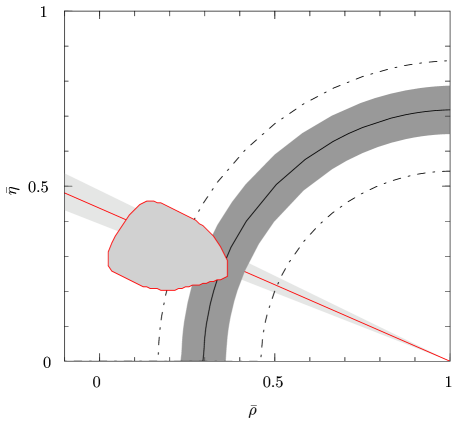
Figure 3: Constraints implied by $R_{0}$ in the ($\bar{\rho},\bar{\eta}$) plane. The experimental value used is $R_{0}=0.007\pm 0.003$ (see text for further explanation). The width of the dark band reflects a $\pm 10\%$ variation of $\xi$ for central $R_{0}$. The dash-dotted lines display the error from $R_{0}$ while $\xi$ is kept at its central value. The region obtained from a standard fit of the unitarity triangle (irregularly shaped area) and the constraint from $\sin 2\beta$ (light shaded band) are overlaid.

For the purpose of illustration we shall assume that the results in [3] and [4] can be interpreted to give

$$B(B^{0}\to\rho^{0}\gamma)=\left(0.30\pm 0.12\right)\cdot 10^{-6}$$ (41)

Here we have combined the average $\rho^{\pm}/\rho^{0}/\omega$ branching ratio from [3] and [4], obtaining $B(B\to(\rho/\omega)\gamma)=(0.64\pm 0.27)\cdot 10^{-6}$. Dividing by $2\,\tau_{B^{+}}/\tau_{B^{0}}$ then gives (41) as an estimate for $B(B^{0}\to\rho^{0}\gamma)$. We use the central value in (1) to compute the experimental ratio

$$R_{0}=\frac{B(B^{0}\to\rho^{0}\gamma)}{B(B^{0}\to K^{*0}\gamma)}=0.007\pm 0.003$$ (42)

Adopting an error of $\pm 10\%$ for the SU(3)-breaking form factor ratio $\xi=1.31\pm 0.13$ and the central value in (42), we obtain the dark shaded band in Fig. 3. Here the full expression (25) is used, without expanding in $\delta a$, and all theoretical parameters besides $\xi$ are kept at their central values. This is justified as the theoretical uncertainty is entirely dominated by $\xi$. For the same constraint, the dash-dotted lines indicate the $1\sigma$ experimental uncertainty from (42) with fixed $\xi=1.3$.

As can be seen, the intersection of the constraints from $R_{0}$ and $\sin 2\beta$ determines the apex ($\bar{\rho},\bar{\eta}$) of the unitarity triangle. For comparison, the standard fit region for the unitarity triangle in the ($\bar{\rho},\bar{\eta}$) plane [29] and the constraint from the experimental measurement of $\sin 2\beta=0.734\pm 0.054$ [30] are also shown in Fig. 3.

We finally note that the information from $R_{0}$ is already becoming comparable with the constraint from the ratio of $B_{d}$ and $B_{s}$ meson mixing frequencies $\Delta M_{B_{d}}$ and $\Delta M_{B_{s}}$ [31]. It is possible that a useful experimental measurement of $R_{0}$ might actually be achieved before the measurement of $\Delta M_{B_{s}}$. Very interesting in this respect is the recent upper bound for $B(B^{0}\to\rho^{0}\gamma)$ from Babar (4). As we have discussed above, the neutral mode is favoured theoretically because of the small impact of annihilation effects. In addition, it turns out that the upper bound for $B(B^{0}\to\rho^{0}\gamma)$ is particularly strong in comparison with the bound for the charged mode (5), even after correcting for an isospin factor of 2 and the $B^{+}/B^{0}$ lifetime difference. We thus prefer to use the neutral mode directly for placing an upper bound on $R_{t}$, rather than the combined result of the three modes $(\rho^{\pm}/\rho^{0}/\omega)\gamma$, which was the choice made in [3]. Using (39), the recent Babar limit (4) together with (1) implies

$$R_{t}<0.82\,\frac{\xi}{1.3}$$ (43)

This is equivalent to

$$\left|\frac{V_{td}}{V_{ts}}\right|<0.18\,\frac{\xi}{1.3}\qquad\qquad|V_{td}|<7.3\cdot 10^{-3}\,\frac{\xi}{1.3}$$ (44)

The bound may be compared with the $2\sigma$ range

$$6.5\cdot 10^{-3}<|V_{td}|<9.5\cdot 10^{-3}$$ (45)

obtained from a standard fit of the unitarity triangle [29]. For $30\%$ SU(3) breaking in the ratio of form factors, $\xi=1.3$, more than half of the range (45) is excluded by (44). Should the amount of SU(3) breaking be less than $30\%$, the bound would be even stronger. An illustration of the Babar bound in the $(\bar{\rho},\bar{\eta})$ plane is given in Fig. 4.

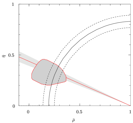
Figure 4: Upper bound on $R_{t}$ (the distance from point $(1,0)$) implied by the Babar limit $B(B^{0}\to\rho^{0}\gamma)<0.4\cdot 10^{-6}$ in the ($\bar{\rho},\bar{\eta}$) plane. The curves correspond (from left to right) to $\xi\equiv F_{K^{*}}/F_{\rho}=1.4$, $1.3$ and $1.2$. The region obtained from a standard fit of the unitarity triangle (irregularly shaped area) and the constraint from $\sin 2\beta$ (light shaded band) are overlaid.

4 $B\to\rho\gamma$ and $B\to\rho l\nu$

As we have seen, the rare decay $B\to\rho\gamma$ is a clean probe of flavour physics, except for the sizable uncertainty in the form factor $F_{\rho}$. Other uncertainties are quite well under control within a treatment of the decay at next-to-leading order in QCD and a leading-order evaluation of power-suppressed annihilation effects. This is the case in particular for the neutral channel $B^{0}\to\rho^{0}\gamma$, where weak-annihilation effects are small. The sensitivity to $F_{\rho}$ can be reduced by taking the ratio of $B\to\rho\gamma$ and $B\to K^{*}\gamma$ branching fractions, as we have discussed in the previous section. Then the impact of long-distance hadronic physics is limited to SU(3) breaking in the ratio $\xi=F_{K^{*}}/F_{\rho}$. While this is certainly an advantage, the exact deviation from the SU(3) limit $\xi=1$ remains at present a significant source of uncertainty.

In this section we discuss a possibility to reduce hadronic uncertainties in a different way, using the ratio of $B\to\rho l\nu$ and $B\to\rho\gamma$ decay rates. The simplification occurs because relations exist between the corresponding form factors in the large energy limit. Since only $B\to\rho$ transitions are involved, the problems with SU(3) breaking are avoided and only isospin symmetry needs to be assumed, which should be valid to within a few percent. The existence of relations between the form factors in the large energy limit and their potential usefulness for phenomenology were first pointed out in [32]. The results of [32] were put on a field theoretical basis within the soft-collinear effective theory (SCET) and extended to higher order in QCD [33, 22, 21]. These relations were applied to extract information on the form factor in $B\to K^{*}\gamma$ for use in other channels such as $B\to K^{*}l^{+}l^{-}$ [34]. Previously, the authors of [35] have investigated the possibility to relate $B\to\rho l\nu$ in a certain region of phase space with $B\to K^{*}\gamma$. This suggestion is similar in spirit to our proposal, but the analysis of [35] was based only on the heavy quark limit, instead of the full large energy relations from [32], and was still affected by SU(3) breaking. In addition, our discussion also includes short-distance QCD corrections at next-to-leading order.

The differential decay rate for $B\to\rho l\nu$ is given by

$$\frac{d^{2}\Gamma(B\to\rho l\nu)}{ds\,dz}=c^{2}_{\rho}\frac{G^{2}_{F}m^{5}_{B}}{256\pi^{3}}|V_{ub}|^{2}w^{1/2}\left[\frac{(1-z)^{2}}{2}H^{2}_{+}+\frac{(1+z)^{2}}{2}H^{2}_{-}+(1-z^{2})H^{2}_{0}\right]$$ (46)

Here

$$w\equiv w(s,r)=1+s^{2}+r^{2}-2s-2r-2sr$$ (47)

and

$$z=\cos\theta\qquad\qquad s=\frac{q^{2}}{m^{2}_{B}}\qquad\qquad r=\frac{m^{2}_{\rho}}{m^{2}_{B}}\approx 0.021$$ (48)

where $q^{2}$ is the dilepton invariant mass and $\theta$ is the angle between the momenta of the neutrino and the $B$ meson in the dilepton centre-of-mass frame. Equivalently, $\theta$ is the angle between the charged-lepton momentum and the direction anti-parallel to the $B$ momentum in this frame. The same definition of $\theta$ is valid for $B\to\rho l\nu$ with either a positive or a negative charged lepton. The kinematical range for $s$ and $z$ is

$$0\leq s\leq(1-\sqrt{r})^{2}\qquad-1\leq z\leq 1$$ (49)

The $H_{i}\equiv H_{i}(s)$ are helicity form factors. They can be expressed in terms of the vector and axial vector form factors $V(s)$, $A_{1}(s)$ and $A_{2}(s)$ as

$$H_{\pm} = \sqrt{s}\left[(1+\sqrt{r})A_{1}\mp\frac{\sqrt{w}}{1+\sqrt{r}}\,V\right]$$ (50)

$$H_{0} = \frac{1}{2\sqrt{r}}\left[(1-s-r)(1+\sqrt{r})A_{1}-\frac{w}{1+\sqrt{r}}A_{2}\right]$$ (51)

where we use the conventions of [32] for $V$, $A_{1}$, $A_{2}$, which, in particular, are positive real quantities.

The CP-averaged decay rate for $B\to\rho\gamma$ can be written as

$$\Gamma(B\to\rho\gamma)=\frac{G^{2}_{F}\alpha m^{3}_{B}m^{2}_{b}}{32\pi^{4}}(1-r)^{3}\,|V_{td}V_{tb}|^{2}\,|a^{c}_{7}(\rho\gamma)|^{2}\,c^{2}_{\rho}F^{2}_{\rho}$$ (52)

where we have used the approximation, explained in the previous section, that corresponds to neglecting the term $\sim{\rm Re}\,\delta a$ in (31). As we have seen, this is a very good approximation for $B^{0}\to\rho^{0}\gamma$. If a more accurate treatment is desired, or the analysis should be applied to $B^{\pm}\to\rho^{\pm}\gamma$, the following discussion can be generalized in a straightforward way using the complete expression based on (16). Combining (46) and (52) we find for the case of neutral $B$ mesons

$$k(s,z)\left|\frac{V_{ud}V_{ub}}{V_{td}V_{tb}}\right|^{2}=\frac{4\alpha}{\pi}\,\frac{m^{2}_{b}}{m^{2}_{B}}\,\frac{(1-r)^{3}|V_{ud}|^{2}|a^{c}_{7}(\rho\gamma)|^{2}}{B(B^{0}\to\rho^{0}\gamma)}\ \frac{dB(B^{0}\to\rho l\nu)}{ds\,dz}$$ (53)

Here $B^{0}\to\rho l\nu$ can be either one of the two channels $B^{0}\to\rho^{+}l^{-}\bar{\nu}$ or $B^{0}\to\rho^{-}l^{+}\nu$ and $l$ may be an electron or a muon. The hadronic quantity $k$ is defined as

$$k(s,z)=w(s,r)^{1/2}\left[\frac{(1-z)^{2}}{2}\frac{H^{2}_{+}}{F^{2}_{\rho}}+\frac{(1+z)^{2}}{2}\frac{H^{2}_{-}}{F^{2}_{\rho}}+(1-z^{2})\frac{H^{2}_{0}}{F^{2}_{\rho}}\right]$$ (54)

The differential branching ratio and the function $k$ in (53) may be replaced by their integrated versions

$$\Delta B(\bar{s},\epsilon)=\int_{0}^{\bar{s}}ds\int_{1-\epsilon}^{1}dz\frac{dB(B^{0}\to\rho l\nu)}{ds\,dz}\qquad K(\bar{s},\epsilon)=\int_{0}^{\bar{s}}ds\int_{1-\epsilon}^{1}dz\,k(s,z)$$ (55)

where

$$0\leq\bar{s}\leq s_{max}\equiv(1-\sqrt{r})^{2}\approx 0.73\qquad\quad 0\leq\epsilon\leq 2$$ (56)

such that the fully integrated branching fraction for $B^{0}\to\rho l\nu$ is given by $\Delta B(s_{max},2)$.

The relation (53) allows us to determine the CKM parameter

$$\left|\frac{V_{ud}V_{ub}}{V_{td}V_{tb}}\right|^{2}=\frac{\bar{\rho}^{2}+\bar{\eta}^{2}}{(1-\bar{\rho})^{2}+\bar{\eta}^{2}}$$ (57)

in terms of observable $B\to\rho\gamma$ and $B\to\rho l\nu$ branching fractions, known quantities, and the hadronic function $k$. The main virtue of this expression is that in the large energy limit hadronic form factors cancel in the ratios $H_{\pm}/F_{\rho}$. This is not the case for $H_{0}/F_{\rho}$, but its contribution can be suppressed by selecting events in the vicinity of $z=1$. As a consequence, (53) can be turned into a theoretically clean expression for the determination of the CKM ratio in (57).

In the large energy limit the form factors $H_{\pm}$, $H_{0}$ and $F_{\rho}$ can be written in terms of just two independent form factors $\zeta_{\perp}(s)$ and $\zeta_{\parallel}(s)$ using [32]

$$A_{1}(s)=\frac{1-s+r}{1+\sqrt{r}}\zeta_{\perp}(s)\qquad\quad V(s)=(1+\sqrt{r})\,\zeta_{\perp}(s)$$ (58)

$$A_{2}(s)=(1+\sqrt{r})\left[\zeta_{\perp}(s)-\frac{2\sqrt{r}}{1-s+r}\zeta_{\parallel}(s)\right]\qquad\quad F_{\rho}\equiv T_{1}(0)=\zeta_{\perp}(0)$$ (59)

Together with (50), (51) these relations imply

$$H_{\pm}(s) = \sqrt{s}\left[\,1-s+r\mp\sqrt{w}\,\right]\,\zeta_{\perp}(s)$$ (60)

$$H_{0}(s) = \sqrt{r}(1+s-r)\,\zeta_{\perp}(s)+\frac{w}{1-s+r}\,\zeta_{\parallel}(s)$$ (61)

These results are valid in the heavy-quark limit and the limit of large energy of the recoiling $\rho$-meson

$$E_{\rho}=\frac{m_{B}}{2}(1-s+r)$$ (62)

In this approximation the ratio $H_{+}/H_{-}$ is independent of hadronic form factors. For not too large values of $s$ this ratio is strongly suppressed, $H_{+}/H_{-}={\cal O}(r)$. More importantly, also $H_{-}(s)$ and $F_{\rho}$ depend on the same form factor $\zeta_{\perp}(s)$, which is to be evaluated at $s=0$ in the latter case. As a consequence, we may write

$$\frac{H^{2}_{-}(s)}{F^{2}_{\rho}}=4s\,(1+b_{1}s+\ldots)$$ (63)

expanding the form factor ratio in a Taylor series. The leading term in this ratio for small $s$ is largely free of hadronic uncertainties in the large energy limit. The higher-order corrections only depend on the shape of $\zeta_{\perp}(s)$, not on its absolute normalization, and can in principle be determined from a fit to the shape of the observed spectrum in $s$. The coefficient $b_{1}$ is related to the slope of $\zeta_{\perp}$ and can be written as

$$b_{1}=2\left(\frac{\zeta^{\prime}_{\perp}(0)}{\zeta_{\perp}(0)}-\frac{1}{1-r}\right)$$ (64)

When fitting the ratio in (63) to the experimental spectrum, other parametrizations for the shape may, of course, be chosen. The Taylor series $1+b_{1}s+\ldots$ could be replaced for instance by the pole form $1/(1-\beta_{1}s)^{2}$, or a combination of the two.

In [33] the corrections of order $\alpha_{s}$ have been computed to the relations between form factors in the large energy limit. There is no relative correction between $A_{1}$ and $V$ to all orders in $\alpha_{s}$ [36]. Therefore the correction of the ratio $V/F_{\rho}$ given in [33] also applies to $H_{-}/F_{\rho}$. Taking these effects into account, the leading term ($4s$) in (63) is modified to

$$\frac{H^{2}_{-}(s)}{F^{2}_{\rho}}=4s\,\left(1+\frac{2\alpha_{s}(\mu_{1})}{3\pi}\left[1+2\ln\frac{\mu_{1}}{m_{b}}\right]-\frac{\alpha_{s}(\mu_{2})}{3\pi}\frac{\Delta F_{\perp}}{V(0)}(1+\sqrt{r})\right)$$ (65)

where the first term with $\alpha_{s}(\mu_{1})\approx 0.22$ refers to the vertex correction and the second with $\alpha_{s}(\mu_{2})\approx 0.34$ to the hard spectator interaction. The usual renormalization scheme of the form factor $F_{\rho}$, adopted in this paper and used in (65), corresponds to the $\overline{MS}$ scheme with anticommuting $\gamma_{5}$ (NDR). Numerically, the QCD correction factor amounts to $(1-(0.15\pm 0.10))$ using the estimates in [33]. The dominant uncertainty comes from $\Delta F_{\perp}$, which depends on properties of the $B$-meson light-cone wave function. This quantity is poorly known at present, but improvements should be possible in the future and would lead to a reduction in the uncertainty.

It is interesting to compare the above analysis with the results for the form factors obtained using the method of light-cone QCD sum rules [17]. With the form factors computed in [17] one finds

$$\frac{H^{2}_{-}(s)}{F^{2}_{\rho}}=4.25s\,(1+0.59s+0.65s^{2}+\ldots)$$ (66)

The leading term agrees very well with the prediction at leading order in the large energy limit (63). Taking the QCD corrections into account according to (65), the prediction for this term is typically about $15\%$ lower. On the other hand, the result in (66) has an uncertainty of about $30\%$ [17]. Nevertheless, the general level of agreement of the sum rule calculations, which include subleading corrections in $1/m_{b}$, with the large energy limit, is consistent with the assumption that power corrections are of moderate size.

In contrast to $H_{\pm}$, the longitudinal form factor $H_{0}$ is dominated by $\zeta_{\parallel}$, which is not cancelled in the ratio $H_{0}/F_{\rho}$. The third term in (54) can still be estimated theoretically, but will be affected by larger uncertainites. As mentioned above, in order to reduce its importance a cut on the angular variable $z$ may be imposed, restricting $z$ to be in the vicinity of $+1$ or $-1$. The latter case is not interesting, since it would strongly suppress the $H_{-}$ contribution, leaving only the contribution from $H_{+}$, which is very small. Parametrizing the cut below $z=1$ by $\epsilon$ as defined in (55) and performing the angular integration, we find for $K(\bar{s},\epsilon)$

$$K(\bar{s},\epsilon)=\int^{\bar{s}}_{0}ds\,\sqrt{w}\left[\frac{\epsilon^{3}}{6}\frac{H^{2}_{+}}{F^{2}_{\rho}}+\left(2\epsilon-\epsilon^{2}+\frac{\epsilon^{3}}{6}\right)\frac{H^{2}_{-}}{F^{2}_{\rho}}+\left(\epsilon^{2}-\frac{\epsilon^{3}}{3}\right)\frac{H^{2}_{0}}{F^{2}_{\rho}}\right]$$ (67)

The full angular range is obtained for $\epsilon=2$ and in this case all three $\epsilon$-dependent coefficients become equal to $4/3$. For small $\epsilon$, on the other hand, a strong hierarchy exists, which is clearly visible in (67). The contribution from $H_{0}$ is suppressed with respect to the $H_{-}$-term by a factor of $\epsilon/2$, that is by one order of magnitude for $\epsilon=0.2$. The corresponding suppression of the $H_{+}$-term is even by a factor of $\epsilon^{2}/12$, in addition to the fact that $H_{+}/H_{-}$ is already small for moderate values of $s$. The contribution from $H_{+}$ is therefore entirely negligible in the following discussion.

Neglecting all terms of ${\cal O}(\epsilon^{3})$, (67) simplifies to

$$K(\bar{s},\epsilon)=\int^{\bar{s}}_{0}ds\,\sqrt{w}\left[2\epsilon\,\frac{H^{2}_{-}}{F^{2}_{\rho}}+\epsilon^{2}\frac{H^{2}_{0}-H^{2}_{-}}{F^{2}_{\rho}}\right]$$ (68)

The validity of the large energy limit, with the model-independent normalization of $H^{2}_{-}/F^{2}_{\rho}$ in (63), (65), requires moderate values of $s$. Enhancing this term in (67) requires small $\epsilon$. As a typical example one may concentrate on the part of phase space defined by $\bar{s}=0.4$ and $\epsilon=0.2$. The relative number of $B^{0}\to\rho l\nu$ events in this region ($0\leq s\leq 0.4$, $0.8\leq z\leq 1$) is given by

$$\frac{K(0.4,0.2)}{K(s_{max},2)}\approx 0.064$$ (69)

For this estimate we have evaluated $K(\bar{s},\epsilon)$ employing the form factors from [17]. A measurement of $B\to\rho l\nu$ has been reported by CLEO [37],

$$B(B^{0}\to\rho l\nu)=(2.17\pm 0.73)\cdot 10^{-4}$$ (70)

and BaBar [38]:

$$B(B^{0}\to\rho l\nu)=(2.57\pm 0.79)\cdot 10^{-4}$$ (71)

The effective branching ratio of $B\to\rho l\nu$ events in the above region of phase space would then be about $10^{-5}$.

The first term in (68) is determined by the measured shape of the $s$-distribution and the model-independent normalization in (63), (65). The small correction from the second term in (68) could either be estimated theoretically, or be isolated in the data by varying $\epsilon$. With the form factors from [17] we have for instance

$$K(0.4,\epsilon)=0.57\,\epsilon+0.25\,\epsilon^{2}$$ (72)

Once $K(\bar{s},\epsilon)$ is known, the measured values of $\Delta B(\bar{s},\epsilon)$ (55) and $B(B^{0}\to\rho^{0}\gamma)$ determine the CKM quantity in (57) using (53). This CKM ratio provides us with an interesting constraint in the ($\bar{\rho},\bar{\eta}$) plane, which is illustrated in Fig. 5 for a hypothetical measurement of $|V_{ud}V_{ub}/V_{td}|^{2}=0.16\pm 0.04$.

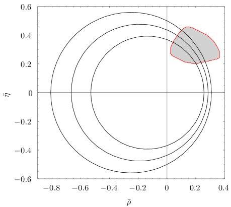
Figure 5: Constraints in the ($\bar{\rho},\bar{\eta}$) plane implied by $|V_{ud}V_{ub}/V_{td}|^{2}=0.16\pm 0.04$. For comparison, the standard fit region is indicated by the shaded area.

We observe that the constraint is quite stringent, in particular in the important region corresponding to the standard fit results, and even for the rather moderate precision of $\pm 25\%$.

5 Isospin Breaking in $B\to V\gamma$

The CP averaged isospin breaking ratio can be defined as

$$\Delta(V\gamma)=\frac{\Gamma(B^{0}\to V^{0}\gamma)-v\Gamma(B^{\pm}\to V^{\pm}\gamma)}{\Gamma(B^{0}\to V^{0}\gamma)+v\Gamma(B^{\pm}\to V^{\pm}\gamma)}$$ (73)

with $v=1$ for $V=K^{*}$ and $v=1/2$ for $V=\rho$. This ratio has a reduced sensitivity to the nonperturbative form factors. As already discussed, in our approximations, isospin breaking is generated by weak annihilation contributions. Kagan and Neubert found a large effect from the penguin operator $Q_{6}$ on the isospin asymmetry $\Delta(K^{*}\gamma)$ [39]. Our prediction $\Delta(K^{*}\gamma)=(3.9^{+3.1}_{-1.9})\%$ (see [14]) is in agreement with the experimental results (Belle in [2], Babar [40])

$$\Delta(K^{*}\gamma) = +0.034\pm 0.044\pm 0.026\pm 0.025\ \ \ \ {\rm(Belle)}$$ (74)

$$\Delta(K^{*}\gamma) = +0.051\pm 0.044\pm 0.023\pm 0.024\ \ \ \ {\rm(Babar)}$$ (75)

Here the errors are statistical, systematic and from the $B^{+}/B^{0}$ production ratio.

For $B\to\rho\gamma$ we find a strong dependence of the isospin asymmetry on the angle $\gamma$ of the unitarity triangle. As seen in Fig. 6,

Figure 6: The isospin-breaking asymmetries $\Delta(\rho\gamma)$ and $\Delta(K^{*}\gamma)$ as a function of the CKM angle $\gamma$ with (solid) and without (dashed) the inclusion of QCD penguin operator effects.

the $\gamma$ dependence is in particular pronounced for the zero crossing of $\Delta(\rho\gamma)$ around $\gamma=60^{\circ}$, the value favoured by the standard UT fits.

Once a measurement of both the charged and neutral $B\to\rho\gamma$ modes is available, the isospin-asymmetry $\Delta(\rho\gamma)$ can be used to constrain the unitarity triangle. For the purpose of illustration we plot in Fig. 7, in addition to the $R_{0}$ and $\sin 2\beta$ bands shown already in Fig. 3, the implication of an assumed measurement of $\Delta(\rho\gamma)_{exp}=0$, which would correspond to the Standard Model prediction for a CKM angle $\gamma=60^{\circ}$. The dominant theoretical uncertainty comes from the hadronic parameter $\lambda_{B}$ and from the variation of the renormalization scale.

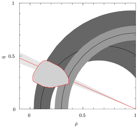
Figure 7: Same as Fig. 3 including the implication of a measurement of $\Delta(\rho\gamma)_{exp}=0$ (curved band on the right). The width of the band reflects the theoretical uncertainties from varying the hadronic parameter $\lambda_{B}$ and the renormalization scale $\mu$. (The effect of isospin breaking in the form factors is neglected here.)

6 $B\to\omega\gamma$

In this section we briefly consider the decay $\bar{B}^{0}\to\omega^{0}\gamma$ and discuss differences to the related mode $\bar{B}^{0}\to\rho^{0}\gamma$. We consider $\rho^{0}$ and $\omega^{0}$ as pure isospin-1 and isospin-0 modes, respectively, and neglect $\rho-\omega$ mixing. We use the convention $\omega^{0}=\frac{u\bar{u}+d\bar{d}}{\sqrt{2}}$, $\rho^{0}=\frac{u\bar{u}-d\bar{d}}{\sqrt{2}}$.

To leading order in the heavy-quark limit and next-to-leading order in $\alpha_{s}$ both the $\rho^{0}$ and $\omega^{0}$ meson in $B\to V\gamma$ are produced from a $d\bar{d}$ pair. Therefore, to get the $\bar{B}\to\omega^{0}\gamma$ decay amplitude, we can use the one for $\bar{B}\to\rho^{0}\gamma$ with obvious replacements for the vector meson decay constant, mass, LCDA and form factor in the factorization coefficients $a_{7}^{u/c}(\rho^{0}\gamma)$ [6, 12, 14]. The relevant input parameters for all the decay modes are compiled in Table 1.

A few comments are in order. The best known input parameter for the vector mesons is the mass, which can be found in the Review of Particle Physics [41]. Using $\tau$-decay data and the purely leptonic decay modes of $\rho^{0}$ and $\omega^{0}$ one can extract the respective decay constants $f_{\rho,\,\omega}$ with negligible uncertainty [26]. The other vector meson parameters, such as the $B\to V$ form factors were taken from QCD sum rule estimates [17]. We take the same values for the $\omega$ and $\rho$ mesons, which should be a reasonable assumption, even though this equality could be broken by Zweig-rule violating effects. The latter are, however, suppressed by $1/N_{c}$. For instance, the decay constants $f_{\rho}$ and $f_{\omega}$ differ by $10\%$.

In [6, 14] we included weak annihilation contributions to $B\to V\gamma$ although they are suppressed by one power of $\Lambda_{\mathrm{Q}CD}/m_{b}$. The reason for including these power-suppressed contributions was that they are in part enhanced by large Wilson coefficients, they are calculable in QCD factorization and they can be used to estimate isospin-breaking effects. For $B\to\omega\gamma$ annihilation contributions are also calculable and they are the source of specific differences (apart from form factors) between $\bar{B}^{0}\to\rho^{0}\gamma$ and $\bar{B}^{0}\to\omega^{0}\gamma$. Those are due to the fact that $\rho^{0}$ and $\omega^{0}$ are isospin-0 and isospin-1 states, respectively. In the following we will use the notation of section 4.5 in [14]. If, in figure 8,

Figure 8: Annihilation contribution to the $\bar{B}\to V\gamma$ decay. The dominant mechanism for operators $Q_{1\ldots 4}$ is the radiation of the photon from the light quark in the $B$ meson, as shown. This amplitude is suppressed by one power of $\Lambda_{QCD}/m_{b}$, but it is still calculable in QCD factorization. Radiation of the photon from the remaining three quark lines is suppressed by $(\Lambda_{QCD}/m_{b})^{2}$ for operators $Q_{1\ldots 4}$. For operators $Q_{5,6},$ however, radiation from the final state quarks is again of order $\Lambda_{QCD}/m_{b}$.

the photon emission is from the light quark in the $B$ meson, the annihilation amplitude contains

$$b^{V}=\frac{2\pi^{2}}{F_{V}}\frac{f_{B}m_{V}f_{V}}{m_{B}m_{b}\lambda_{B}}$$ (76)

whereas the $Q_{5,6}$ insertion with the photon emitted from one of the vector meson constituent quarks leads to

$$d^{V}_{\stackrel{{\scriptstyle(-)}}{{v}}}=-\frac{4\pi^{2}}{F_{V}}\frac{f_{B}f_{V}^{\perp}}{m_{B}m_{b}}\int_{0}^{1}\frac{dv}{\stackrel{{\scriptstyle(-)}}{{v}}}\Phi_{V}^{\perp}(v)$$ (77)

The annihilation coefficients for $\bar{B}^{0}\to\omega^{0}\gamma$ then are

$$a_{ann}^{u}(\omega^{0}\gamma) = Q_{d}\left[+a_{2}b^{\omega}-2b^{\omega}(a_{4}+a_{6})+a_{4}b^{\omega}+a_{6}(d^{\omega}_{v}+d^{\omega}_{\bar{v}})\right]$$ (78)

$$a_{ann}^{c}(\omega^{0}\gamma) = Q_{d}\left[-2b^{\omega}(a_{4}+a_{6})+a_{4}b^{\omega}+a_{6}(d^{\omega}_{v}+d^{\omega}_{\bar{v}})\right]$$ (79)

The difference compared to $a_{ann}^{u/c}(\rho^{0}\gamma)$ is the sign change of the $a_{2}$ contribution and the additional isospin-0 contribution $-2b^{\omega}(a_{4}+a_{6})$.

Numerically the $\omega$ and $\rho^{0}$ annihilation coefficients are given by

$$a_{ann}^{u}(\omega\gamma) = -\frac{1}{3}\Big{[}\begin{array}[t]{cccc}+0.0268&+0.0281&-0.0060&+0.0446\\ +a_{2}b^{\omega}&\!\!-2b^{\omega}(a_{4}+a_{6})\!\!&+a_{4}b^{\omega}&+a_{6}(d^{\omega}_{v}+d^{\omega}_{\bar{v}})\end{array}\Big{]}=-0.0312$$ (82)

$$a_{ann}^{u}(\rho^{0}\gamma) = -\frac{1}{3}\Big{[}\begin{array}[t]{ccc}-0.0296&-0.0066&+0.0446\\ -a_{2}b^{\rho}&+a_{4}b^{\rho}&+a_{6}(d^{\rho}_{v}+d^{\rho}_{\bar{v}})\end{array}\Big{]}=-0.0028$$ (85)

For comparison we quote the corresponding numbers for the $\rho^{-}\gamma$ channel

$$a_{ann}^{u}(\rho^{-}\gamma)=\frac{2}{3}\Big{[}\begin{array}[t]{cccc}+0.2902&-0.0066&-0.0112&+0.0223\\ +a_{1}b^{\rho}&+a_{4}b^{\rho}&+Q_{s}/Q_{u}a_{6}d^{\rho}_{v}&+a_{6}d^{\rho}_{\bar{v}}\end{array}\Big{]}=+0.1965$$ (86)

where the annihilation component is considerably larger. This has to be compared with $a_{7}^{u}(\omega\gamma)=a_{7}^{u}(\rho^{0}\gamma)=-0.4154-0.0685i$, to which the annihilation coefficients are added. For central values of all input parameters, $\mu=m_{b}$, and our default choice for the CKM angle $\gamma=58^{\circ}$, we get the following CP-averaged branching ratios:

$$\bar{B}(B^{0}\to\omega\gamma) = 0.84\cdot 10^{-6}$$ (87)

$$\bar{B}(B^{0}\to\rho^{0}\gamma) = 0.81\cdot 10^{-6}$$ (88)

$$\bar{B}(B^{\pm}\to\rho^{\pm}\gamma) = 1.81\cdot 10^{-6}$$ (89)

Within the parametric and theoretical uncertainties the $B^{0}\to\omega\gamma$ and $B^{0}\to\rho\gamma$ branching ratios can be considered equal, neglecting any possile difference in the respective form factors.

7 Conclusions and Outlook

We have studied constraints on the CKM unitarity triangle from observables in the exclusive radiative decays $B\to K^{*}\gamma$, $B\to\rho\gamma$, and $B\to\omega\gamma$, as well as the exclusive semileptonic decay $B\to\rho l\nu$. Within the framework of QCD factorization we have worked at next-to-leading order in $\alpha_{s}$ to leading order in the heavy-quark limit. Power corrections from weak annihilation have also been included. Important information on the unitarity-triangle parameters $\bar{\rho}$ and $\bar{\eta}$ can be obtained from the ratio $R_{0}$ of the neutral $B^{0}\to\rho^{0}\gamma$ and $B^{0}\to K^{*0}\gamma$ branching ratios. This ratio measures to very good approximation the side $R_{t}$ of the standard unitarity triangle. Annihilation effects are negligible in this case. The theoretical uncertainty in the relation to $R_{t}$ comes in essence solely from the form-factor ratio $\xi=F_{K^{*}}/F_{\rho}$, which differs from unity only because of SU(3)-breaking effects. Using the latest bound on $B(B^{0}\to\rho^{0}\gamma)$ from Babar we find $R_{t}<0.81\,(\xi/1.3)$ or $|V_{td}|<7.3\cdot 10^{-3}\,(\xi/1.3)$ (see also Fig. 4).

Similar constraints in the $(\bar{\rho},\bar{\eta})$ plane can be obtained from the isospin asymmetry $\Delta(\rho\gamma)$ once a measurement of this quantity is available.

We propose to gain complementary information in the $(\bar{\rho},\bar{\eta})$ plane through the $B\to\rho l\nu$ and $B\to\rho\gamma$ decay rates, which can be related to the CKM parameter $|V_{ud}V_{ub}/(V_{td}V_{tb})|^{2}$. For events where the momenta of the neutrino and the $B$ meson are parallel in the dilepton centre-of-mass frame, this relation is free of hadronic form factors in the large energy limit. This allows a theoretically clean determination of the above CKM ratio. We have shown that even a moderate experimental precision can yield a stringent constraint in the $(\bar{\rho},\bar{\eta})$ plane.

Finally, we have calculated the annihilation effects in the $B\to\omega\gamma$ decay amplitude which turn out to be very small.

An improved determination of the $B\to V$ form factors and, in particular, the form-factor ratio $\xi$, remains an important task for the future. More precise experimental measurements, specifically the individual measurements of $B(B^{0}\to\rho^{0}\gamma)$ and $B(B^{+}\to\rho^{+}\gamma)$ are eagerly awaited. These measurements can lead to results on $R_{t}$ competitive with those from $B_{s}$-$\bar{B}_{s}$ mixing. An experimental analysis of the differential $B\to\rho l\nu$ to $B\to\rho\gamma$ decay rate ratio can circumvent the form-factor related uncertainties to a large extent and will thus be of particular interest.

Acknowledgements: S.W.B. wants to thank Thorsten Feldmann for helpful discussion of the $B\to\omega$ form factor. This research was supported in part by the National Science Foundation under Grant PHY-0355005.

References

- [1] T. Hurth, Rev. Mod. Phys. 75 (2003) 1159.
- [2] T. E. Coan et al. [CLEO Collaboration], Phys. Rev. Lett. 84 (2000) 5283; B. Aubert et al. [BABAR Collaboration], hep-ex/0407003. M. Nakao et al. [BELLE Collaboration], Phys. Rev. D 69 (2004) 112001.
- [3] B. Aubert et al. [BABAR Collaboration], hep-ex/0408034.
- [4] H.Y.G. Yang [BELLE Collaboration], talk at ICHEP 2004, Beijing, China, August 2004.
- [5] M. Beneke, G. Buchalla, M. Neubert and C. T. Sachrajda, Phys. Rev. Lett. 83 (1999) 1914, Nucl. Phys. B 591 (2000) 313.
- [6] S. W. Bosch and G. Buchalla, Nucl. Phys. B 621 (2002) 459.
- [7] M. Beneke, T. Feldmann and D. Seidel, Nucl. Phys. B 612 (2001) 25.
- [8] A. Ali and A. Y. Parkhomenko, Eur. Phys. J. C 23 (2002) 89.
- [9] H. H. Asatrian, H. M. Asatrian and D. Wyler, Phys. Lett. B 470 (1999) 223; C. Greub, H. Simma and D. Wyler, Nucl. Phys. B 434 (1995) 39 [Erratum-ibid. B 444 (1995) 447].
- [10] N. Deshpande et al., Phys. Rev. Lett. 59 (1987) 183.
- [11] A. Ali and E. Lunghi, Eur. Phys. J. C 26 (2002) 195; A. Ali, E. Lunghi and A. Y. Parkhomenko, Phys. Lett. B 595 (2004) 323.
- [12] T. Hurth and E. Lunghi, eConf C0304052 (2003) WG206.
- [13] S. W. Bosch and G. Buchalla, eConf C0304052 (2003) WG203; S. W. Bosch, hep-ph/0310317.
- [14] S. W. Bosch, Ph.D. Thesis, MPI-PHT-2002-35, hep-ph/0208203.
- [15] C. Greub, T. Hurth and D. Wyler, Phys. Rev. D 54 (1996) 3350;
- [16] A. J. Buras, A. Czarnecki, M. Misiak and J. Urban, Nucl. Phys. B 631 (2002) 219.
- [17] P. Ball and V. M. Braun, Phys. Rev. D 58 (1998) 094016.
- [18] D. Becirevic, talk at the Ringberg Phenomenology Workshop on Heavy Flavours, Ringberg Castle, Tegernsee, May 2003.
- [19] P. Ball, hep-ph/0308249.
- [20] M. Beneke and T. Feldmann, Nucl. Phys. B 685 (2004) 249.
- [21] B. O. Lange and M. Neubert, Nucl. Phys. B 690 (2004) 249.
- [22] C. W. Bauer, S. Fleming, D. Pirjol and I. W. Stewart, Phys. Rev. D 63 (2001) 114020; C. W. Bauer, D. Pirjol and I. W. Stewart, Phys. Rev. D 67 (2003) 071502.
- [23] P. Koppenburg et al. [Belle Collaboration], hep-ex/0403004.
- [24] P. Gambino and M. Misiak, Nucl. Phys. B 611, 338 (2001).
- [25] S. M. Ryan, Nucl. Phys. Proc. Suppl. 106 (2002) 86.
- [26] M. Beneke and M. Neubert, Nucl. Phys. B 675 (2003) 333.
- [27] P. Ball and E. Kou, JHEP 0304 (2003) 029.
- [28] V. M. Braun, D. Y. Ivanov and G. P. Korchemsky, Phys. Rev. D 69 (2004) 034014.
- [29] A. Höcker et al. [CKMfitter], http://ckmfitter.in2p3.fr/; A. Höcker, H. Lacker, S. Laplace and F. Le Diberder, Eur. Phys. J. C 21 (2001) 225; J. Charles et al. [CKMfitter], hep-ph/0406184.
- [30] M. Battaglia et al., proceedings of the Workshop on the Unitarity Triangle (CERN Yellow Report to appear), hep-ph/0304132.
- [31] B. Golob [Belle Collaboration], eConf C030626 (2003) FRAT04.
- [32] J. Charles et al., Phys. Rev. D 60 (1999) 014001.
- [33] M. Beneke and T. Feldmann, Nucl. Phys. B 592 (2001) 3;
- [34] G. Burdman and G. Hiller, Phys. Rev. D 63 (2001) 113008.
- [35] G. Burdman and J. F. Donoghue, Phys. Lett. B 270 (1991) 55.
- [36] R. J. Hill, T. Becher, S. J. Lee and M. Neubert, JHEP 0407 (2004) 081.
- [37] S. B. Athar et al. [CLEO Collaboration], Phys. Rev. D 68 (2003) 072003.
- [38] B. Aubert et al. [BABAR Collaboration], hep-ex/0408068.
- [39] A. L. Kagan and M. Neubert, Phys. Lett. B 539 (2002) 227.
- [40] E. Paoloni [BABAR Collaboration], talk at the Rencontres de Moriond, Electroweak Session, La Thuile, Italy, March 2004; hep-ex/0406083.
- [41] K. Hagiwara et al. [Particle Data Group Collaboration], Phys. Rev. D 66 (2002) 010001.