HEPHY-PUB 789/04 July 2004

FACETS OF THE
SPINLESS SALPETER EQUATION
Wolfgang LUCHA
Institut für Hochenergiephysik,
Österreichische Akademie der Wissenschaften,
Nikolsdorfergasse 18, A-1050 Wien, Austria
Franz F. SCHÖBERL
Institut für Theoretische Physik, Universität Wien,
Boltzmanngasse 5, A-1090 Wien, Austria

Abstract

The spinless Salpeter equation represents the simplest, and most straightforward, generalization of the Schrödinger equation of standard nonrelativistic quantum theory towards the inclusion of relativistic kinematics. Moreover, it can be also regarded as a well-defined approximation to the Bethe–Salpeter formalism for descriptions of bound states in relativistic quantum field theories. The corresponding Hamiltonian is, in contrast to all Schrödinger operators, a nonlocal operator. Because of the nonlocality, constructing analytical solutions for such kind of equation of motion proves difficult. In view of this, different sophisticated techniques have been developed in order to extract rigorous analytical information about these solutions. This review introduces some of these methods and compares their significance by application to interactions relevant in physics.

PACS numbers: 03.65.Ge, 03.65.Pm, 11.10.St

1 Bethe–Salpeter Formalism in the “Instantaneous Approximation”

Within quantum field theory, the appropriate framework for the description of bound states is the Bethe–Salpeter formalism [1]. Therein, all bound states of two particles (in fact, of any two fermionic constituents) are governed by the homogeneous Bethe–Salpeter equation. Here we are interested in a particular well-defined approximation to this formalism, obtained by several simplifying steps:

1. The instantaneous approximation, neglecting any retardation effect, considers all interactions of the (two) bound-state constituents in their static limit.

2. The additional assumption that all the bound-state constituents propagate as free particles with some effective mass $m$ yields the Salpeter equation [2].

3. A disregard of all of their spin degrees of freedom focuses on the treatment of scalar bound particles.

4. In technical respect, the canonical transformation

   $$\mbox{\boldmath{$x$}}\to\lambda\,\mbox{\boldmath{$x$}}\ ,\quad\mbox{\boldmath{$p$}}\to\frac{\mbox{\boldmath{$p$}}}{\lambda}$$ (1)

   of position ($x$) and momentum ($p$) variables casts in the case of particles of equal mass $m$ for a scale factor $\lambda=2$ this approach into one-particle form.

(For more details of the derivation, consult, for instance, Refs. [3, 4, 5] and references therein.) Refraining from the nonrelativistic limit, we get the (nonlocal!) Hamiltonian

$$H=T+V\ .$$ (2)

This operator is composed of the “square-root operator” $T$ of the relativistically correct expression for the kinetic or free energy of a particle of mass $m$ and momentum $\mbox{\boldmath{$p$}},$

$$T=T(\mbox{\boldmath{$p$}})\equiv\sqrt{\mbox{\boldmath{$p$}}^{2}+m^{2}}\ ,$$ (3)

and a (coordinate-dependent) static interaction potential

$$V=V(\mbox{\boldmath{$x$}})\ ;$$

frequently, the potential $V(\mbox{\boldmath{$x$}})$ is assumed to be a central potential that depends merely on the radial coordinate $r$:

$$V=V(r)\ ,\quad r\equiv|\mbox{\boldmath{$x$}}|\ .$$

The eigenvalue equation for this particular Hamiltonian,

$$H\,|\chi_{k}\rangle=E_{k}\,|\chi_{k}\rangle\ ,\quad k=0,1,2,\dots\ ,$$ (4)

defining a complete system of Hilbert-space eigenstates $|\chi_{k}\rangle$ of $H$ corresponding to its (energy) eigenvalues $E_{k},$

$$E_{k}\equiv\frac{\langle\chi_{k}|\,H\,|\chi_{k}\rangle}{\langle\chi_{k}|\chi_{k}\rangle}\ ,\quad k=0,1,2,\dots\ ,$$

is commonly known as the “spinless Salpeter equation.”

2 The Relativistic Virial Theorem

Useful general statements about the solutions of explicit or implicit eigenvalue equations may be proved with the help of virial theorems obtained by generalization [6] of the well-known result of nonrelativistic quantum theory. (Ref. [7] is a brief review of relativistic virial theorems.) For eigenvalue equations of the form (4), the derivations of such virial theorems can be traced back to the (trivial) observation that expectation values taken with respect to given eigenstates $|\chi_{k}\rangle$ of $H$ — or matrix elements taken with respect to arbitrary pairs of degenerate eigenstates, $|\chi_{i}\rangle$ and $|\chi_{j}\rangle,$ of $H,$ i. e., eigenstates satisfying $E_{i}=E_{j}$ — of the commutators $[G,H]$ of the operator $H$ and any other operator $G$ (the domain of which must be assumed to contain the domain of $H$) clearly vanish. Suppressing the subscript that enumerates the eigenstates, this means

$$\langle\chi|\,[G,H]\,|\chi\rangle=0\ .$$ (5)

For the symmetrized, self-adjoint generator of dilations,

$$G\equiv\mbox{$\frac{1}{2}$}\,(\mbox{\boldmath{$x$}}\cdot\mbox{\boldmath{$p$}}+\mbox{\boldmath{$p$}}\cdot\mbox{\boldmath{$x$}})\ ,$$ (6)

and $H$ of the form (2) their commutator $[G,H]$ becomes

$$[G,H]={\rm i}\left[\mbox{\boldmath{$p$}}\cdot\frac{\partial\,T}{\partial\mbox{\boldmath{$p$}}}(\mbox{\boldmath{$p$}})-\mbox{\boldmath{$x$}}\cdot\frac{\partial\,V}{\partial\mbox{\boldmath{$x$}}}(\mbox{\boldmath{$x$}})\right].$$

In this case Eq. (5) yields the master virial theorem [6, 7]

$$\left\langle\chi\left|\,\mbox{\boldmath{$p$}}\cdot\frac{\partial\,T}{\partial\mbox{\boldmath{$p$}}}(\mbox{\boldmath{$p$}})\,\right|\chi\right\rangle=\left\langle\chi\left|\,\mbox{\boldmath{$x$}}\cdot\frac{\partial\,V}{\partial\mbox{\boldmath{$x$}}}(\mbox{\boldmath{$x$}})\,\right|\chi\right\rangle;$$ (7)

this relation expresses the equality of all the expectation values of the momentum-space radial derivative of $T(\mbox{\boldmath{$p$}})$ and the (configuration-space) radial derivative of $V(\mbox{\boldmath{$x$}}),$ it produces the specific virial theorem for a particular $H.$ For any nonrelativistic (Schrödinger) Hamiltonian, i. e.,

$$H=H_{\rm S}=m+\frac{\mbox{\boldmath{$p$}}^{2}}{2\,m}+V(\mbox{\boldmath{$x$}})\ ,$$

Theorem (7) entails, retaining the conventional factor $\mbox{$\frac{1}{2}$},$

$$\left\langle\chi\left|\,\frac{\mbox{\boldmath{$p$}}^{2}}{2\,m}\,\right|\chi\right\rangle=\frac{1}{2}\left\langle\chi\left|\,\mbox{\boldmath{$x$}}\cdot\frac{\partial\,V}{\partial\mbox{\boldmath{$x$}}}(\mbox{\boldmath{$x$}})\,\right|\chi\right\rangle.$$ (8)

For the semirelativistic “spinless-Salpeter” Hamiltonian (2), involving the square-root operator of the relativistic kinetic energy (3), our master virial theorem (7) leads to

$$\left\langle\chi\left|\,\frac{\mbox{\boldmath{$p$}}^{2}}{\sqrt{\mbox{\boldmath{$p$}}^{2}+m^{2}}}\,\right|\chi\right\rangle=\left\langle\chi\left|\,\mbox{\boldmath{$x$}}\cdot\frac{\partial\,V}{\partial\mbox{\boldmath{$x$}}}(\mbox{\boldmath{$x$}})\,\right|\chi\right\rangle.$$ (9)

In the nonrelativistic limit $m\to\infty$ (i. e., for $\mbox{\boldmath{$p$}}^{2}\ll m^{2}$), this spinless-Salpeter relativistic virial theorem, Eq. (9), necessarily reduces to its nonrelativistic counterpart (8). Similarly, the virial theorem for the Dirac equation [8, 9] is easily deduced [7] from our master virial theorem (7).

3 Bounds to Energy Eigenvalues of a Spinless-Salpeter Hamiltonian

The precise determination of eigenvalues of operators is of particular importance for any formulation of quantum theory. Unfortunately, for most cases it is not possible to determine the point spectrum (the set of all eigenvalues) of a given operator analytically. Several powerful tools, however, allow to derive analytic bounds to eigenvalues; applications of these techniques to the spinless-Salpeter operator (2) are reviewed, for instance, in Refs. [10, 11, 12, 13].

3.1 Minimum–maximum principle

The theoretical foundation of any derivation of a system of rigorous upper bounds to the (isolated) eigenvalues of some operator $H$ in Hilbert space and hence the primary tool for any localization of the discrete spectrum of $H$ is the well-known minimum–maximum principle [14, 15, 16]. Its precise formulation is based on several prerequisites:

• Let this operator $H$ be some self-adjoint operator.

• Assume that this operator is bounded from below.

• Define the eigenvalues of $H,$ $E_{k},$ $k=0,1,2,\dots,$ by the eigenvalue equation, with eigenstates $|\chi_{k}\rangle,$

  $$H\,|\chi_{k}\rangle=E_{k}\,|\chi_{k}\rangle\ ,\quad k=0,1,2,\dots\ .$$

• Let these eigenvalues $E_{k}$ be ordered, according to

  $$E_{0}\leq E_{1}\leq E_{2}\leq\cdots\ .$$

• Consider only the eigenvalues $E_{k}$ below the onset of the essential spectrum of the above operator $H.$

• Restrict all considerations to some $d$-dimensional subspace $D_{d}\subset{\cal D}(H)$ of the domain ${\cal D}(H)$ of $H.$

Then this theorem asserts that every eigenvalue $E_{k}$ of $H$ — counting multiplicity of degenerate levels — satisfies

$$E_{k}\leq\displaystyle\sup_{|\psi\rangle\in D_{k+1}}\frac{\langle\psi|\,H\,|\psi\rangle}{\langle\psi|\psi\rangle}\quad\mbox{for all}\ k=0,1,2,\dots\ .$$

In the case of one-dimensional subspaces, that is, $d=1,$ the minimum–maximum theorem reduces to Rayleigh’s principle: the ground-state eigenvalue $E_{0}$ of an operator $H$ is less than, or equal to, every expectation value of $H$:

$$E_{0}\leq\frac{\langle\psi|\,H\,|\psi\rangle}{\langle\psi|\psi\rangle}\ ,\quad|\psi\rangle\in{\cal D}(H)\ .$$

Given some operator inequality satisfied by the operator $H,$ the minimum–maximum principle may be employed to derive, by comparison, upper bounds on the (discrete) eigenvalues of $H,$ provided that a few assumptions hold:

• The operator $H,$ exhibiting all properties required by the minimum–maximum principle, is bounded from above by some other operator called ${\cal O},$ i. e., it is subject to an (operator) inequality of the form

  $$H\leq{\cal O}\ .$$

  Applying both the minimum–maximum principle and this operator inequality, any eigenvalue $E_{k}$ of $H$ must be bounded from above by the supremum of the expectation values of the operator ${\cal O}$ within the $(k+1)$-dimensional subspace $D_{k+1}$ of ${\cal D}(H)$:

  $$E_{k} \equiv \frac{\langle\chi_{k}|\,H\,|\chi_{k}\rangle}{\langle\chi_{k}|\chi_{k}\rangle}$$ (10)

  $$\leq \sup_{|\psi\rangle\in D_{k+1}}\frac{\langle\psi|\,H\,|\psi\rangle}{\langle\psi|\psi\rangle}$$

  $$\leq \sup_{|\psi\rangle\in D_{k+1}}\frac{\langle\psi|\,{\cal O}\,|\psi\rangle}{\langle\psi|\psi\rangle}$$

  $$\quad\mbox{for all}\ k=0,1,2,\dots\ .$$

• All eigenvalues $\widehat{E}_{k}$ of ${\cal O}$ are ordered according to

  $$\widehat{E}_{0}\leq\widehat{E}_{1}\leq\widehat{E}_{2}\leq\cdots\ .$$

• Every $k$-dimensional subspace $D_{k}$ in the chain of inequalities which constitutes Eq. (10) is spanned by the first $k$ eigenvectors of the operator ${\cal O},$ or by precisely those eigenvectors of ${\cal O}$ that correspond to the first $k$ eigenvalues $\widehat{E}_{0},\widehat{E}_{1},\dots,\widehat{E}_{k-1}$ of our ${\cal O}.$ For this case it is very easy to convince oneself that the supremum of all expectation values of the operator ${\cal O}$ over the $(k+1)$-dimensional subspace $D_{k+1}$ is then identical to the eigenvalue $\widehat{E}_{k}$ of ${\cal O}$:

  $$\sup_{|\psi\rangle\in D_{k+1}}\frac{\langle\psi|\,{\cal O}\,|\psi\rangle}{\langle\psi|\psi\rangle}=\widehat{E}_{k}\ .$$

Consequently, an eigenvalue $E_{k},$ $k=0,1,2,\dots,$ of the discrete spectrum of $H(\leq{\cal O})$ is bounded from above by the corresponding eigenvalue $\widehat{E}_{k},$ $k=0,1,2,\dots,$ of ${\cal O}$:

$$E_{k}\leq\widehat{E}_{k}\quad\mbox{for all}\ k=0,1,2,\dots\ .$$

It remains to prove an “appropriate” operator inequality. (Summaries of the idea to find bounds by combining the minimum–maximum principle with reasonable operator inequalities may be found, e. g., in Refs. [17, 12, 13, 18].)

3.2 Analytical upper bounds

3.2.1 The trivial nonrelativistic Schrödinger bound

The inequality $(T-m)^{2}\geq 0$ expressing nothing but the positivity of the square of the operator $T-m$ may be, for $m>0,$ written as an inequality for the kinetic energy $T$:

$$T\leq m+\frac{\mbox{\boldmath{$p$}}^{2}}{2\,m}\ .$$

(The right-hand side is the tangent line to the square root in the relativistic kinetic energy $T$ in the point of contact $\mbox{\boldmath{$p$}}^{2}=0.$) This result proves [17] that $H$ is bounded from above by a nonrelativistic Schrödinger Hamiltonian $H_{\rm S}$:

$$H\leq H_{\rm S}=m+\frac{\mbox{\boldmath{$p$}}^{2}}{2\,m}+V\ .$$

For a pure Coulomb potential $V(r)=-\alpha/r,$ the energy eigenvalues of the Schrödinger Hamiltonian $H_{\rm S}$ depend only on the principal quantum number $n,$ related to both radial and orbital angular-momentum quantum numbers by $n=n_{\rm r}+\ell+1,$ with $n_{\rm r}=0,1,2,\dots,$ $\ell=0,1,2,\dots$:

$$E_{{\rm S},n}=m\left(1-\frac{\alpha^{2}}{2\,n^{2}}\right).$$

3.2.2 A “squared” bound

A relation between the (semirelativistic) Hamiltonian $H$ and a nonrelativistic Schrödinger operator may be found [17] by considering the square $H^{2}$ of $H$ and by realizing that the anticommutator $T\,V+V\,T$ of relativistic kinetic energy $T$ and potential $V$ generated by the square fulfils

$$T\,V+V\,T\leq\mbox{\boldmath{$p$}}^{2}+V^{2}+2\,m\,V\ ,$$

as may be shown [17] by inspecting some consequences of the positivity of the square of the operator $T-m-V$:

$$H^{2} = T^{2}+V^{2}+T\,V+V\,T$$

$$\leq Q\equiv 2\,\mbox{\boldmath{$p$}}^{2}+m^{2}+2\,V^{2}+2\,m\,V\ .$$

With this inequality, the minimum–maximum principle, recalled in Subsect. 3.1, immediately guarantees that the energy eigenvalues $E_{k}$ of $H$ are bounded from above by the square root of the corresponding eigenvalues ${\cal E}_{Q,k}$ of the Schrödinger operator $Q,$ constructed by squaring $H$:

$$E_{k}\leq\sqrt{{\cal E}_{Q,k}}\ ,\quad k=0,1,2,\dots\ .$$

For the case of a pure Coulomb potential $V(r)=-\alpha/r,$ the operator $Q$ has the same structure as the Schrödinger Hamiltonian $H_{\rm S}$ of Subsect. 3.2.1, with $\ell$ replaced by an effective orbital angular momentum quantum number $L$ involving both the usual $\ell$ and the Coulomb coupling, $\alpha$:

$$L\,(L+1)=\ell\,(\ell+1)+\alpha^{2}\ ,\quad\ell=0,1,2,\dots\ .$$ (11)

The set of eigenvalues ${\cal E}_{Q}$ of a “Coulombic” operator $Q,$

$${\cal E}_{Q,N}=m^{2}\left(1-\frac{\alpha^{2}}{2\,N^{2}}\right),$$

is determined by the effective principal quantum number

$$N=n_{\rm r}+L+1\ ,\quad n_{\rm r}=0,1,2,\dots\ .$$

Unfortunately, in the Coulomb case the squared bounds are above, and thus worse than, the Schrödinger bounds.

3.3 Rigorous semianalytical upper bound

We regard an energy bound as semianalytical if it can be derived by an (in general, numerical) optimization of an analytically given expression over a single real variable. Taking advantage, as a straightforward generalization of the (simple) line of argument sketched in Subsect. 3.2.1, of the inequality $(T-\mu)^{2}\geq 0$ requiring an arbitrary real parameter $\mu$ of mass dimension 1 and obviously holding for all self-adjoint $T$ [19] implies, for the kinetic energy,

$$T\leq\frac{\mbox{\boldmath{$p$}}^{2}+m^{2}+\mu^{2}}{2\,\mu}\quad\mbox{for all}\ \mu>0\ .$$

This translates [17] to a set of inequalities for $H,$ each of these involving a Schrödinger-like Hamiltonian, $\widehat{H}_{\rm S}(\mu)$:

$$H\leq\widehat{H}_{\rm S}(\mu)=\frac{\mbox{\boldmath{$p$}}^{2}+m^{2}+\mu^{2}}{2\,\mu}+V\quad\mbox{for all}\ \mu>0\ .$$

The best “Schrödinger-like” upper bound on any energy eigenvalue $E_{k}$ of $H$ is then provided by the minimum of the $\mu$-dependent energy eigenvalues of $\widehat{H}_{\rm S}(\mu),$ $\widehat{E}_{{\rm S},k}(\mu)$:

$$E_{k}\leq\displaystyle\min_{\mu>0}\widehat{E}_{{\rm S},k}(\mu)\ ,\quad k=0,1,2,\dots\ .$$

For a pure Coulomb potential $V(r)=-\alpha/r,$ the energy eigenvalues $\widehat{E}_{{\rm S},n}(\mu)$ of $\widehat{H}_{\rm S}(\mu)$ read, with $n=n_{\rm r}+\ell+1,$

$$\widehat{E}_{{\rm S},n}(\mu)=\frac{1}{2\,\mu}\left[m^{2}+\mu^{2}\left(1-\frac{\alpha^{2}}{n^{2}}\right)\right].$$

Here, minimizing $\widehat{E}_{{\rm S},n}(\mu)$ with respect to $\mu$ entails [17]

$$\min_{\mu>0}\widehat{E}_{{\rm S},n}(\mu)=m\,\sqrt{1-\frac{\alpha^{2}}{n^{2}}}\ .$$

This (exact) upper bound [17] to the energy eigenvalues of the so-called “spinless relativistic Coulomb problem” holds for all those values of the Coulomb coupling $\alpha$ for which the Hamiltonian $H$ with a Coulomb potential can be regarded as a reasonable operator and arbitrary levels of excitation, and for any value of the principal quantum number $n$ it definitely improves the Schrödinger bound:

$$\min_{\mu>0}\widehat{E}_{{\rm S},n}(\mu)<E_{{\rm S},n}\quad\mbox{for}\ \alpha\neq 0\ .$$

Clearly, fixing $\mu=m$ recovers the Schrödinger bounds.

3.4 Exact semianalytical upper and lower bounds from the “envelope technique”

Rigorous semianalytical expressions for both upper and lower bounds to the eigenvalues $E_{n\ell}$ of the Hamiltonian $H$ are found by a geometrical operator comparison in an approach called “envelope theory.” The envelope theory constructs bounds on $E_{n\ell}$ by comparing the spectrum of $H$ with the one of a conveniently formulated “tangential Hamiltonian” $\widetilde{H}$ involving some “basis potential” $h(r),$

$$\widetilde{H}=\sqrt{m^{2}+\mbox{\boldmath{$p$}}^{2}}+c\,h(r)+\mbox{const.}\ ,\quad c>0\ ,$$

for which sufficient spectral information (i. e., either the exact eigenvalues or suitable bounds on these) is known. Let $V(r)$ be a smooth transformation $V=g(h)$ of $h(r),$ with definite convexity of $g(h).$ After optimization with respect to the point of contact of $V(r)$ and the tangential potential, this technique produces bounds on $E_{n\ell}$: lower bounds for $g(h)$ convex $(g^{\prime\prime}>0),$ and upper bounds for $g(h)$ concave $(g^{\prime\prime}<0).$ Suppressing for the moment the quantum numbers $n\ell,$ all these bounds on $E$ may be cast into a common generic form [20, 21, 22, 23, 24, 25] with the individual bounds discriminated by a dimensionless parameter, $P$:

$$E\approx\min_{r>0}\left[\sqrt{m^{2}+\frac{1}{r^{2}}}+V(P\,r)\right].$$ (12)

Here, that cryptic sign of approximate equality indicates that for any definite convexity of $g(h)$ all expressions on the right-hand side represent a lower bound for a convex $g(h)$ and an upper bound for a concave $g(h).$ The value of the parameter $P$ used in Eq. (12) is determined by the algebraic structure of the interaction potential $V(r),$ and by its convexity with respect to the basis potential, $h(r)$:

• The spinless relativistic Coulomb problem posed by $V(r)=-\alpha/r$ is well-defined if its coupling $\alpha$ is constrained to $\alpha<2/\pi$ [26]. The bottom of the corresponding spectrum of $H$ (or, its ground-state energy eigenvalue, $E_{0}$) is bounded from below by

  $$E_{0}\geq m\,\sqrt{1-\frac{\alpha^{2}}{P^{2}}}\ ,$$

  with the lower-bound parameter $P$ given either by $P=2/\pi$ for $\alpha$ fulfilling $0\leq\alpha<2/\pi$ [26], or by

  $$P\equiv P(\alpha)=\sqrt{\mbox{$\frac{1}{2}$}\left(1+\sqrt{1-4\,\alpha^{2}}\right)}$$

  for $0\leq\alpha\leq\mbox{$\frac{1}{2}$},$ which obviously covers the range

  $$P(\mbox{$\frac{1}{2}$})=\mbox{$\frac{1}{\sqrt{2}}$}\leq P(\alpha)\leq P(0)=1\ ,$$

  as derived by weakening [21, 22, 23, 25] an improved lower bound to $E_{0}$ valid only for $0\leq\alpha\leq\frac{1}{2}$ [27].

  If $V(r)$ is a convex transform $V=g(h),$ $g^{\prime\prime}>0,$ of the Coulomb potential $h(r)=-1/r,$ the above envelope approximation generates a lower bound [21, 22, 23, 25] on the ground-state eigenvalue $E_{0}$ (on the entire spectrum) of the Hamiltonian $H$ for any choice of the Coulomb lower-bound parameter $P.$

  Clearly, the quoted upper bounds on the Coulomb coupling $\alpha$ apply also to any “effective” Coulomb coupling in $\widetilde{H}.$ Consequently, they translate into a constraint on all coupling constants introduced by the interaction potential $V(r)$ under investigation. (An example for these restrictions enforced by the Coulomb menace will be given in Subsect. 3.7.2.)

• For $V(r)$ a concave transform $V=g(h),$ $g^{\prime\prime}<0,$ of the harmonic-oscillator potential $h(r)=r^{2},$ a straightforward application of the above envelope approximation yields upper bounds [21, 22, 23, 25] to all the eigenvalues $E_{n\ell}$ of the Hamiltonian $H;$ the parameter $P$ for a given energy level identified by quantum numbers $n\ell$ is, in this case, related to the explicitly algebraically known eigenvalues ${\cal E}_{n\ell}$ of the (nonrelativistic) Schrödinger operator $\mbox{\boldmath{$p$}}^{2}+r^{2}$:

  $$P\equiv P_{n\ell}(2)=\mbox{$\frac{1}{2}$}\,{\cal E}_{n\ell}=2\,n+\ell-\mbox{$\frac{1}{2}$}\ .$$

• For $V(r)$ a concave transform $V=g(h),$ $g^{\prime\prime}<0,$ of the linear potential $h(r)=r,$ the application of a “generalized” envelope approximation provides upper bounds [23, 25] to all eigenvalues $E_{n\ell}$ of $H$ if the parameters $P$ which characterize the energy levels are given, in terms of the eigenvalues ${\cal E}_{n\ell}$ of the nonrelativistic Schrödinger operator $\mbox{\boldmath{$p$}}^{2}+r,$ by

  $$P\equiv P_{n\ell}(1)=2\left(\mbox{$\frac{1}{3}$}\,{\cal E}_{n\ell}\right)^{3/2}\ ;$$ (13)

  the parameter values $P_{n\ell}(1)$ corresponding to the lowest-lying energy levels can be found in Table 1 (for more details see, for instance, Refs. [20, 21, 22, 23]).

Table 1: Numerical values of the parameter $P_{n\ell}(1)$ used in the linear-potential-based lower envelope bounds and defined in Eq. (13) for the lowest-lying energy levels $n\ell.$

$n$	$\ell$	$P_{n\ell}(1)$
1	0	1.37608
2	0	3.18131
3	0	4.99255
4	0	6.80514
5	0	8.61823
1	1	2.37192
2	1	4.15501
3	1	5.95300
4	1	7.75701
5	1	9.56408
1	2	3.37018
2	2	5.14135
3	2	6.92911
4	2	8.72515
5	2	10.52596

       $n$ $\ell$ $P_{n\ell}(1)$ 1 3 4.36923 2 3 6.13298 3 3 7.91304 4 3 9.70236 5 3 11.49748 1 4 5.36863 2 4 7.12732 3 4 8.90148 4 4 10.68521 5 4 12.47532 1 5 6.36822 2 5 8.12324 3 5 9.89276 4 5 11.67183 5 5 13.45756

If the potential $V(r)$ is the sum of several distinct terms,

$$V(r)=\sum_{i}V_{i}(r)\ ,\quad V_{i}(r)=c_{i}\,h_{i}(r)\ ,$$

where every component problem defined by the operator

$$\sqrt{m^{2}+\mbox{\boldmath{$p$}}^{2}}+c_{i}\,h_{i}(r)$$

supports, for a sufficiently large $c_{i},$ a discrete eigenvalue $E_{i,0}$ at the bottom of its spectrum and information about the lowest energy eigenvalue, $E_{i,0},$ is available, all these pieces of information can be combined to a lower bound to $E_{0}$ [24]; for sums of pure power-law terms ${\rm sgn}(q)\,r^{q},$

$$V_{\rm PL}(r)=\sum_{q}a(q)\,{\rm sgn}(q)\,r^{q}\ ,$$ (14)

where the coefficients $a(q)$ of the pure power-law terms, ${\rm sgn}(q)\,r^{q},$ in the potential are positive, that is, $a(q)\geq 0,$ and do not vanish all, this yields the “sum lower bound”

$$E_{0}\geq\min_{r>0}\left[\sqrt{m^{2}+\frac{1}{r^{2}}}+\sum_{q}a(q)\,{\rm sgn}(q)\,(\underline{P}(q)\,r)^{q}\right]$$

provided that some set of lower-bound parameters $\underline{P}(q)$ can be derived such that, whenever $V(r)$ consists of just one single component, the above inequality yields either the corresponding exact ground-state energy eigenvalue or, at least, a rigorous lower bound to this latter quantity:

• For Coulomb components, that is, $h_{i}(r)=-1/r,$ $\underline{P}(-1)$ is the Coulomb lower-bound parameter $P.$

• For linear components, that is, $h_{i}(r)=r,$ $\underline{P}(1)$ is derived from the lowest eigenvalue ${\cal E}_{0}$ of $\sqrt{\mbox{\boldmath{$p$}}^{2}}+r,$

  $$\underline{P}(1)=\mbox{$\frac{1}{4}$}\,{\cal E}_{0}^{2}=1.2457\ .$$

It is straightforward to (try to) generalize these envelope techniques from the simpler one-body case summarized in this review to systems composed of arbitrary numbers of relativistically moving interacting particles described by a semirelativistic spinless Salpeter equation [28, 29, 30]. At least for the particular case of all harmonic-oscillator potentials $V(r)=c\,r^{2}$ with $c>0$ the generalized upper bounds presented in Subsect. 3.3 and the envelope upper bounds can be shown to be equivalent to each other [23].

3.5 Rayleigh–Ritz (variational) technique

An immediate consequence of the minimum–maximum principle is the “Rayleigh–Ritz (variational) technique:”

• Introduce the restriction $\widehat{H}$ of some operator $H$ to a subspace $D_{d}$ by orthogonal projection $P$ to $D_{d}$:

  $$\left.\widehat{H}\equiv H\right|_{D_{d}}:=P\,H\,P\ .$$

• Identify all $d$ eigenvalues $\widehat{E}_{k},$ $k=0,1,\dots,d-1,$ of the restricted operator $\widehat{H}$ as the solutions of the eigenvalue equation of $\widehat{H}$ for the eigenstates $|\widehat{\chi}_{k}\rangle$:

  $$\widehat{H}\,|\widehat{\chi}_{k}\rangle=\widehat{E}_{k}\,|\widehat{\chi}_{k}\rangle\ ,\quad k=0,1,\dots,d-1\ .$$

• Let these eigenvalues $\widehat{E}_{k}$ be ordered, according to

  $$\widehat{E}_{0}\leq\widehat{E}_{1}\leq\cdots\leq\widehat{E}_{d-1}\ .$$

Then every (discrete) eigenvalue $E_{k}$ of $H$ — if counting the multiplicity of degenerate levels — is bounded from above by the eigenvalue $\widehat{E}_{k}$ of the restricted operator $\widehat{H}$:

$$E_{k}\leq\widehat{E}_{k}\quad\mbox{for all}\ k=0,1,\dots,d-1\ .$$

If that $d$-dimensional subspace $D_{d}$ is spanned by any set of $d$ (of course, linearly independent) basis vectors $|\psi_{k}\rangle,$ $k=0,1,\dots,d-1,$ the eigenvalues $\widehat{E}_{k}$ can immediately be determined, by the diagonalization of the $d\times d$ matrix

$$\left(\langle\psi_{i}|\,\widehat{H}\,|\psi_{j}\rangle\right),\quad i,j=0,1,\dots,d-1\ ,$$

that is, as the $d$ roots of the characteristic equation of $\widehat{H},$

$$\det\left(\langle\psi_{i}|\,\widehat{H}\,|\psi_{j}\rangle-\widehat{E}\,\langle\psi_{i}|\psi_{j}\rangle\right)=0\ ,$$

$$i,j=0,1,\dots,d-1\ .\,$$

To establish this, expand any eigenvector $|\widehat{\chi}_{k}\rangle$ of $\widehat{H}$ over the basis $\{|\psi_{i}\rangle,\ i=0,1,\dots,d-1\}$ of the subspace $D_{d}.$

3.6 Variational upper bounds

The quality achieved by the variational solution of some eigenvalue problem depends decisively on the definition of the trial subspace $D_{d}$ employed by the Rayleigh–Ritz technique briefly sketched in Subsect. 3.5: enlarging $D_{d}$ to higher dimensions $d$ or choosing a more sophisticated basis $\{|\psi_{i}\rangle,\ i=0,1,\dots,d-1\}$ which spans $D_{d}$ will, in general, increase the accuracy of the obtained solutions.

For spherically symmetric (central) potentials $V(r),$ that is, for all potentials which depend only on the radial coordinate $r\equiv|\mbox{\boldmath{$x$}}|,$ a convenient and thus rather popular choice for the basis vectors $\{|\psi_{i}\rangle,\ i=0,1,\dots,d-1\}$ is that one the configuration-space representation of which involves the complete orthogonal system of generalized Laguerre polynomials [31, 32, 12, 13] — cf. Appendix A.

In the one-dimensional case [33] realized in the notation of Appendix A if all quantum numbers $k=\ell=m=0,$ the Laguerre basis collapses to just a single basis vector:

$$\psi(\mbox{\boldmath{$x$}})\equiv\psi_{0,00}(\mbox{\boldmath{$x$}})=\sqrt{\frac{\mu^{3}}{\pi}}\,\exp(-\mu\,r)\ ,\quad\mu>0\ .$$

With a trial state $|\psi\rangle$ represented by this exponential and the trivial (nevertheless fundamental) general inequality

$$\frac{|\langle\psi|\,{\cal O}\,|\psi\rangle|}{\langle\psi|\psi\rangle}\leq\sqrt{\frac{\langle\psi|\,{\cal O}^{2}\,|\psi\rangle}{\langle\psi|\psi\rangle}}\ ,$$

which holds for any self-adjoint, but otherwise arbitrary, operator ${\cal O}$ (${\cal O}^{\dagger}={\cal O}$), Rayleigh’s principle entails, after optimization with respect to the variational parameter $\mu,$ for a Coulomb potential $V(r)=-\alpha/r$ the upper bound

$$E_{0}\leq m\,\sqrt{1-\alpha^{2}}\ ;$$

this is identical to the “generalized” upper energy bound on the ground-state or $n=1$ eigenvalue of the Coulomb operator $H$ found by different reasoning in Subsect. 3.3.

3.7 Application to illustrative interactions

Let us appreciate the above bounds’ beauty at examples.

3.7.1 Trivial “testing ground:” Coulomb potential

Our first example clearly must be the Coulomb potential

$$V(r)=-\frac{\alpha}{r}\ ,\quad\alpha>0\ ;$$

this potential arises from the exchange of some massless boson between the interacting objects. Therefore it is of particular interest in many areas of physics. Its effective interaction strength is given by a coupling $\alpha,$ identical to the fine structure constant in electrodynamics. We study

• the somewhat naive nonrelativistic (Schrödinger) upper bound given in Subsect. 3.2.1, equivalent to a tangent line to the relativistic kinetic operator $T,$

• the upper bound of Subsect. 3.2.2, constructed by considering just the square of the Hamiltonian $H,$

• the semianalytical upper bound of Subsect. 3.3, as derived by generalizing the idea of Subsect. 3.2.1,

• all three envelope bounds of Subsect. 3.4, namely,

  • the harmonic-oscillator-based upper bound,

  • the upper bound involving a linear potential,

  • the lower bound obtained by “loosening” an absolute lower bound on the spectrum of the “semirelativistic Coulomb operator” $H,$ and

• the “Rayleigh–Ritz” upper bound of Subsect. 3.6.

For the Coulomb potential under study, the optimization required by the envelope bounds (12) may be performed analytically, yielding a result of precisely the same form as the generalized upper bounds derived in Subsect. 3.3, or as the squared upper bounds proved in Subsect. 3.2.2:

$$E_{0}(P)\approx m\,\sqrt{1-\frac{\alpha^{2}}{P^{2}}}\ ,$$ (15)

where for the ground state characterized by the quantum numbers $n=1,$ $\ell=0$ the (single) parameter $P$ is given,

• for the “Coulomb lower bound” (Subsect. 3.4), by

  $$P\equiv P_{\rm C}=P(\alpha)=\sqrt{\mbox{$\frac{1}{2}$}\left(1+\sqrt{1-4\,\alpha^{2}}\right)}\ ,$$

• for the generalized upper bound (Subsect. 3.3), by

  $$P\equiv P_{\rm G}=n=1\ ,$$

• for the “linear upper bound” (Subsect. 3.4), as can be simply read off from the first row in Table 1, by

  $$P\equiv P_{\rm L}=P_{10}(1)=1.37608\ ,$$

• for the “squared upper bound” (Subsect. 3.2.2), in accordance with the solution of Eq. (11) for $L,$ by

  $$P\equiv P_{\rm Q}=\sqrt{2}\,N=\frac{1+\sqrt{1+4\,\alpha^{2}}}{\sqrt{2}}\ ,$$

• and, in the case of the “harmonic-oscillator upper bound” (Subsect. 3.4), from the $P_{n\ell}(2)$ results, by

  $$P\equiv P_{\rm H}=P_{10}(2)=\mbox{$\frac{3}{2}$}\ .$$

It is a very trivial observation that, for fixed values of the Coulomb coupling, the ground-state energy bounds (15) are (monotone) increasing with increasing parameter $P$:

$$\frac{\partial\,E_{0}(P)}{\partial P}\geq 0\ .$$

Thus it is straightforward to convince oneself that all the Coulomb ($E_{\rm C}$), generalized ($E_{\rm G}$), nonrelativistic ($E_{\rm N}$), linear ($E_{\rm L}$), squared ($E_{\rm Q}$) and harmonic-oscillator ($E_{\rm H}$) bounds on the ground-state energy eigenvalue $E_{0}$ of the semirelativistic Coulomb Hamiltonian $H$ have to satisfy

$$E_{\rm C}\leq E_{0}\leq E_{\rm G}\leq E_{\rm N}\leq E_{\rm L}\leq E_{\rm Q}\leq E_{\rm H}$$

$$\mbox{for}\ \alpha\leq\alpha_{0}\equiv\sqrt{\mbox{$\frac{3}{8}$}\left(3-2\,\sqrt{2}\right)}\ ,$$

$$E_{\rm C}\leq E_{0}\leq E_{\rm G}\leq E_{\rm N}\leq E_{\rm L}\leq E_{\rm H}\leq E_{\rm Q}$$

$$\mbox{for}\ \alpha\geq\alpha_{0}\equiv\sqrt{\mbox{$\frac{3}{8}$}\left(3-2\,\sqrt{2}\right)}\ ,$$

taking into account the crossing of the upper bounds $E_{\rm H}$ and $E_{\rm Q}$ at $\alpha_{0}^{2}=\frac{3}{8}\,(3-2\,\sqrt{2}),$ i. e., $E_{\rm Q}(\alpha_{0})=E_{\rm H}(\alpha_{0}).$

For Coulomb-like interactions the only dimensional quantity among the parameters of this theory is the mass $m$ of the interacting particles. Consequently, in this case all energy eigenvalues are proportional to $m$: the energy scale is set by $m.$ The ratio $E_{k}/m$ is a universal function of the coupling $\alpha;$ w. l. o. g. it thus suffices to fix $m=1.$

Figure 1 compares for the ground state ($n_{\rm r}=\ell=0$) of the spinless relativistic Coulomb problem the various bounds to the lowest energy eigenvalue, $E_{0},$ listed at the beginning of this subsection. Inspecting Fig. 1, we note:

• the squared, harmonic-oscillator, and linear upper bounds are numerically comparable to each other;

• likewise the nonrelativistic and generalized upper bounds are close to each other for all couplings $\alpha;$

• using a Laguerre trial space of dimension $d=25,$ the Rayleigh–Ritz variational upper bound can be expected to come already pretty close to the exact eigenvalue $E_{0}$ — which, in turn, clearly indicates that it is highly desirable to find improvements for the lower bounds, in particular for large couplings $\alpha$ (this stimulated, e. g., the analysis of Ref. [34]).

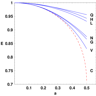
Figure 1: Both upper (full lines) and lower (dashed line) bounds on the ground-state energy eigenvalue (E) of the semirelativistic Hamiltonian $H$ with Coulomb potential $V(r)=-a/r$ as a function of the Coulomb coupling, $a,$ for the squared (Q), harmonic-oscillator (H), linear (L), nonrelativistic (N), generalized (G), variational (V) and Coulomb (C) [using the “optimized” $P(a)$] approaches.

3.7.2 Coulomb-plus-linear (or “funnel”) potential

Within the field of elementary particle physics, quantum chromodynamics (QCD) is generally accepted to be that relativistic quantum field theory that describes all strong interactions between quarks and gluons by assigning the so-called “colour” degrees of freedom to these particles. In the instantaneous approximation inherent to all of the QCD-inspired quark potential models developed for the purely phenomenological description of experimentally observed hadrons, as bound states of constituent quarks, the strong forces are assumed to derive from an effective potential generating the bound states (this description of hadrons within the framework of quark potential models involving either nonrelativistic or relativistic kinematics is reviewed, for instance, in Refs. [3, 35].) The prototype of all “realistic,” that is, phenomenologically acceptable (static) interquark potentials $V(r)$ consists of the sum of

• a Coulomb contribution generated by a one-gluon exchange between quark bound-state constituents (dominating the potential at short distances $r$) and

• a linear term including all nonperturbative effects (that dominates the potential at large distances $r$).

The resulting interaction potential $V(r)$ is characterized by a “funnel-type” Coulomb-plus-linear form; therefore it is called the Coulomb-plus-linear, or funnel, potential. Upon factorizing off a constant $v,$ which spans the range $0<v\leq 1$ in order to parametrize an overall interaction strength, we (prefer to) analyze this potential in the form

$$V(r)=-\frac{c_{1}}{r}+c_{2}\,r=v\left(-\frac{a}{r}+b\,r\right).$$ (16)

Clearly, given the overall coupling strength $v,$ the actual shape of this potential is fixed by the ratio of the positive parameters $a>0$ and $b>0;$ the coupling constants that enter, on the one hand, in the general expression (14) for sums of pure power-law terms and, on the other hand, in our funnel potential (16) must be identified according to

$$a(-1) \equiv c_{1}\equiv a\,v>0\ ,$$

$$a(1) \equiv c_{2}\equiv b\,v>0\ .$$

In view of the lack of fully analytical bounds we explore

• the three “basic” envelope bounds of Subsect. 3.4, distinguished by the adopted basis potential, viz.,

  • the upper bound from a harmonic oscillator,

  • the upper bound involving a linear potential,

  • the lower bound due to a Coulomb potential,

• the envelope sum lower bound, derived in the sum approximation recalled by Subsect. 3.4, as well as

• the “Rayleigh–Ritz” upper bound of Subsect. 3.6.

For definiteness, let us fix the potential parameters $a$ and $b$ to $a=0.2,$ $b=0.5.$ As done in the Coulomb-potential example (in Subsect. 3.7.1) in order to take advantage of upper and lower bounds, we investigate the ground-state energy $E_{0}.$ The basic envelope bounds are computed by application of Eq. (12), for the appropriate parameter $P$:

• for the “harmonic-oscillator upper bound” we use

  $$P\equiv P_{\rm H}=P_{10}(2)=\mbox{$\frac{3}{2}$}\ ;$$

• for the “linear upper bound” we find from Table 1

  $$P\equiv P_{\rm L}=P_{10}(1)=1.37608\ ;$$

• for the “Coulomb lower bound,” in order to derive the maximum value $P$ consistent with $0<v\leq 1,$ we are forced to evaluate that “Coulomb coupling constant constraint” mentioned in Subsect. 3.4, in its form [22, 23] fixed by our funnel potential (16),

  $$c_{1}+\frac{P^{4}}{1-P^{2}}\frac{c_{2}}{m^{2}}\leq P\,\sqrt{1-P^{2}}\ ,$$

  for the maximum values of $c_{1}$ and $c_{2},$ which gives

  $$P\equiv P_{\rm C}=0.728112397\quad\mbox{for}\ m=1\ .$$

The “sum lower bound” is extracted from the expression given explicitly in Subsect. 3.4 for power-law potentials by insertion of the lower-bound parameters $\underline{P}(q=\pm 1)$:

• the Coulomb lower-bound parameter $P(\alpha)$ leads, for the relevant maximum coupling $\alpha=a=0.2,$ in the Coulomb term of the sum approximation to

  $$\underline{P}(-1)=P(\alpha)=P(a)=0.9789063\ ;$$

• the lower-bound parameter required for any linear part of sum potentials is copied from Subsect. 3.4,

  $$\underline{P}(1)=1.2457\ .$$

As before, the Rayleigh–Ritz or variational upper bound is found in a trial space of dimension $d=25$ spanned by the generalized Laguerre basis (summarized in App. A).

Figure 2 depicts the bounds to the lowest eigenvalue $E_{0}$ of $H$ as function of the overall coupling strength $v$ in the funnel potential (16). Remarkably, variational upper and sum lower bounds now restrict $E_{0}$ to a narrow band.

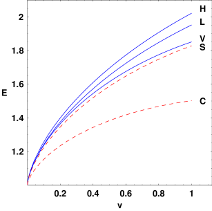
Figure 2: Three upper (full lines) and two lower (dashed lines) bounds on the ground-state energy eigenvalue (E) of the semirelativistic Hamiltonian $H$ with the so-called funnel potential $V(r)=v\,(-a/r+b\,r),$ where $a=0.2,$ $b=0.5,$ $m=1.$ These include: the harmonic-oscillator (H), linear (L) and variational (V) upper bounds and the sum-approximation (S) and Coulomb (C) lower bounds.

4 Approximate Solutions: Quality

Having determined — for instance, by application of the Rayleigh–Ritz technique sketched in Subsect. 3.5 — for some $k=0,1,2,\dots$ the state $|\widehat{\chi}_{k}\rangle\in D_{d}$ corresponding to any upper bound $\widehat{E}_{k}$ on the exact eigenvalue $E_{k}$ of $H,$ one question immediately arises: how closely resembles the approximate solution $|\widehat{\chi}_{k}\rangle$ the exact eigenstate $|\chi_{k}\rangle?$

Standard criteria, such as the (relative) distance between $\widehat{E}_{k}$ and true $E_{k},$ or the overlap of approximate and exact eigenstates, require the knowledge of the exact solution. In contrast to this, the virial theorem (Sect. 2) represents an indicator for the accuracy of approximate eigenstates that merely uses information provided by the variational approach: Since all eigenstates of $H$ satisfy any relation of the form (5), a significant imbalance in Eq. (7) reveals that this approximation is far from optimum [36, 37, 23]. Of course, because of the involvement (5) of the dilation generator (6) in the derivation of Eq. (7), any variational solution found by minimization of expectation values of $H$ with respect to the scale transformations, or dilations, (1) will necessarily satisfy our master virial theorem (7).

5 Summary, Concluding Remarks

The various efficient approaches presented here allow to analyze the semirelativistic Hamiltonians of the spinless Salpeter equation analytically; this is crucial for general considerations that aim to answer questions of principle, like operator boundedness. For numerical methods, see, for instance, Refs. [38, 39, 10] and the references therein.

Appendix A The Generalized Laguerre Basis

Assume every basis function of $L_{2}(R^{3})$ to factorize into a function of the radial variable and the angular term. Its configuration-space representation has the general form

$$\psi_{k,\ell m}(\mbox{\boldmath{$x$}})=\Phi_{k,\ell}(r)\,{\cal Y}_{\ell m}(\Omega_{r})\ ,\quad r\equiv|\mbox{\boldmath{$x$}}|\ ;$$

the spherical harmonics ${\cal Y}_{\ell m}(\Omega)$ for angular momentum $\ell$ and projection $m$ depend on the solid angle $\Omega\equiv(\theta,\phi)$ and satisfy a well-known orthonormalization condition:

$$\int{\rm d}\Omega\,{\cal Y}^{\ast}_{\ell m}(\Omega)\,{\cal Y}_{\ell^{\prime}m^{\prime}}(\Omega)=\delta_{\ell\ell^{\prime}}\,\delta_{mm^{\prime}}\ .$$

The most popular choice [31, 32, 12, 13] for the basis states which span the Hilbert space $L_{2}(R^{+})$ of [with the weight $w(x)=x^{2}$] square-integrable functions $f(x)$ on the positive real line $R^{+}$ — which is the Hilbert space of radial trial functions $\Phi_{k,\ell}(r)$ — involves the generalized Laguerre polynomials $L_{k}^{(\gamma)}(x),$ for parameter $\gamma$ [40, 41]:

$$\Phi_{k,\ell}(r)=N_{k,\ell}^{(\mu,\beta)}\,r^{\ell+\beta-1}\exp(-\mu\,r)\,L_{k}^{(2\,\ell+2\,\beta)}(2\,\mu\,r)\ ;$$

these generalized Laguerre polynomials for parameter $\gamma$ are orthogonal polynomials, defined by the power series

$$L_{k}^{(\gamma)}(x)=\sum_{t=0}^{k}\,(-1)^{t}\left(\begin{array}[]{c}k+\gamma\\ k-t\end{array}\right)\frac{x^{t}}{t!}\ ,\quad k=0,1,\dots\ ,$$

and orthonormalized with weight function $x^{\gamma}\exp(-x)$:

$$\int\limits_{0}^{\infty}{\rm d}x\,x^{\gamma}\exp(-x)\,L_{k}^{(\gamma)}(x)\,L_{k^{\prime}}^{(\gamma)}(x)$$

$$=\frac{\Gamma(\gamma+k+1)}{k!}\,\delta_{kk^{\prime}}\ ,\quad k,k^{\prime}=0,1,\dots\ .$$

The basis states defined by the generalized-Laguerre choice for the radial basis functions $\Phi_{k,\ell}(r)$ involve two parameters, both of which may be subsequently adopted for variational purposes: $\mu$ (with the dimension of mass) and $\beta$ (dimensionless); requirements of normalizability of our basis states constrain the parameters to the ranges

$$0<\mu<\infty\ ,\quad-1<2\,\beta<\infty\ .$$

Therein, the orthonormality of the generalized Laguerre polynomials, inherent to their definition, is equivalent to the orthonormality of the radial basis functions $\Phi_{k,\ell}(r)$:

$$\int\limits_{0}^{\infty}{\rm d}r\,r^{2}\,\Phi_{k,\ell}(r)\,\Phi_{k^{\prime},\ell}(r)=\delta_{kk^{\prime}}\ ,\quad k,k^{\prime}=0,1,\dots\ ;$$

this condition fixes the normalization constant $N_{k,\ell}^{(\mu,\beta)}$ to

$$N_{k,\ell}^{(\mu,\beta)}=\sqrt{\frac{(2\,\mu)^{2\,\ell+2\,\beta+1}\,k!}{\Gamma(2\,\ell+2\,\beta+k+1)}}\ .$$

Fortunately the assumed factorization of every basis function persists in its momentum-space representation:

$$\widetilde{\psi}_{k,\ell m}(\mbox{\boldmath{$p$}})=\widetilde{\Phi}_{k,\ell}(p)\,{\cal Y}_{\ell m}(\Omega_{p})\ ,\quad p\equiv|\mbox{\boldmath{$p$}}|\ .$$

Analytical statements about Hamiltonians that involve a kinetic-energy operator nonlocal in configuration space, such as a relativistic square root (3), are facilitated by an explicit knowledge of the momentum-space basis states. One of the great advantages of the generalized-Laguerre basis is the availability of its analytic Fourier transform.

For all factorizations into radial and angular parts, as consequence of the Fourier transformation acting on the Hilbert space $L_{2}(R^{3})$ of the square-integrable functions on the three-dimensional space $R^{3},$ the radial parts of all basis functions that represent the chosen basis vectors in configuration space and momentum space, respectively, are related by so-called Fourier–Bessel transformations:

$$\Phi_{k,\ell}(r) = {\rm i}^{\ell}\,\sqrt{\frac{2}{\pi}}\int\limits_{0}^{\infty}{\rm d}p\,p^{2}\,j_{\ell}(p\,r)\,\widetilde{\Phi}_{k,\ell}(p)\ ,$$

$$\widetilde{\Phi}_{k,\ell}(p) = (-{\rm i})^{\ell}\,\sqrt{\frac{2}{\pi}}\int\limits_{0}^{\infty}{\rm d}r\,r^{2}\,j_{\ell}(p\,r)\,\Phi_{k,\ell}(r)\ ,$$

$$\quad\mbox{for all}\ k=0,1,\dots,\ \ell=0,1,\dots\ ;$$

the angular-integration remnants $j_{n}(z)$ ($n=0,\pm 1,\dots$) label the spherical Bessel functions of the first kind [40]. For the generalized-Laguerre basis under consideration, these radial basis functions become in momentum space

$$\widetilde{\Phi}_{k,\ell}(p) = N_{k,\ell}^{(\mu,\beta)}\,\frac{(-{\rm i})^{\ell}\,p^{\ell}}{2^{\ell+1/2}\,\Gamma\left(\ell+\frac{3}{2}\right)}$$

$$\times \sum_{t=0}^{k}\,\frac{(-1)^{t}}{t!}\left(\begin{array}[]{c}k+2\,\ell+2\,\beta\\ k-t\end{array}\right)$$

$$\times \frac{\Gamma(a_{t,\ell;\beta})\,(2\,\mu)^{t}}{(p^{2}+\mu^{2})^{a_{t,\ell;\beta}/2}}$$

$$\times F\left(\frac{a_{t,\ell;\beta}}{2},-\frac{\beta+t}{2};\ell+\frac{3}{2};\frac{p^{2}}{p^{2}+\mu^{2}}\right),$$

with the hypergeometric series $F(u,v;w;z)$, defined, in terms of the gamma function $\Gamma,$ by the power series [40]

$$F(u,v;w;z)$$

$$=\frac{\Gamma(w)}{\Gamma(u)\,\Gamma(v)}\,\sum_{n=0}^{\infty}\,\frac{\Gamma(u+n)\,\Gamma(v+n)}{\Gamma(w+n)}\,\frac{z^{n}}{n!}\ ,$$

and the simplifying abbreviation $a_{t,\ell;\beta}\equiv 2\,\ell+\beta+t+2.$

Clearly, the momentum-space radial basis functions $\widetilde{\Phi}_{k,\ell}(p)$ have to satisfy the orthonormalization condition

$$\int\limits_{0}^{\infty}{\rm d}p\,p^{2}\,\widetilde{\Phi}_{k,\ell}^{\ast}(p)\,\widetilde{\Phi}_{k^{\prime},\ell}(p)=\delta_{kk^{\prime}}\ ,\quad k,k^{\prime}=0,1,\dots\ .$$

References

- [1] E. E. Salpeter and H. A. Bethe, Phys. Rev. 84 (1951) 1232.
- [2] E. E. Salpeter, Phys. Rev. 87 (1952) 328.
- [3] W. Lucha, F. F. Schöberl, and D. Gromes, Phys. Rep. 200 (1991) 127.
- [4] J. Resag et al., Nucl. Phys. A 578 (1994) 397 [nucl-th/9307026].
- [5] T. Kopaleishvili, Phys. Part. Nucl. 32 (2001) 560 [hep-ph/0101271].
- [6] W. Lucha and F. F. Schöberl, Phys. Rev. Lett. 64 (1990) 2733.
- [7] W. Lucha and F. F. Schöberl, Mod. Phys. Lett. A 5 (1990) 2473.
- [8] V. Fock, Z. Phys. 63 (1930) 855.
- [9] M. Brack, Phys. Rev. D 27 (1983) 1950.
- [10] W. Lucha and F. F. Schöberl, in: Proc. Int. Conf. on Quark Confinement and the Hadron Spectrum, edited by N. Brambilla and G. M. Prosperi (World Scientific, River Edge (N. J.), 1995) p. 100 [hep-ph/9410221].
- [11] W. Lucha and F. F. Schöberl, in: Proc. XIth Int. Conf. Problems of Quantum Field Theory, editors: B. M. Barbashov, G. V. Efimov, and A. V. Efremov (Joint Institute f. Nuclear Research, Dubna, 1999) p. 482 [hep-ph/9807342].
- [12] W. Lucha and F. F. Schöberl, Int. J. Mod. Phys. A 14 (1999) 2309 [hep-ph/9812368].
- [13] W. Lucha and F. F. Schöberl, Fizika B 8 (1999) 193 [hep-ph/9812526].
- [14] M. Reed and B. Simon, Methods of Modern Mathematical Physics IV: Analysis of Operators (Academic Press, New York, 1978) Section XIII.1.
- [15] A. Weinstein and W. Stenger, Methods of Intermediate Problems for Eigenvalues – Theory and Ramifications (Academic Press, New York, 1972) Chapters 1 and 2.
- [16] W. Thirring, A Course in Mathematical Physics 3: Quantum Mechanics of Atoms and Molecules (Springer, New York/Wien, 1990) Section 3.5.
- [17] W. Lucha and F. F. Schöberl, Phys. Rev. A 54 (1996) 3790 [hep-ph/9603429].
- [18] W. Lucha and F. F. Schöberl, J. Math. Phys. 41 (2000) 1778 [hep-ph/9905556].
- [19] A. Martin, Phys. Lett. B 214 (1988) 561.
- [20] R. L. Hall, W. Lucha, and F. F. Schöberl, J. Phys. A 34 (2001) 5059 [hep-th/0012127].
- [21] R. L. Hall, W. Lucha, and F. F. Schöberl, J. Math. Phys. 42 (2001) 5228 [hep-th/0101223].
- [22] R. L. Hall, W. Lucha, and F. F. Schöberl, Int. J. Mod. Phys. A 17 (2002) 1931 [hep-th/0110220].
- [23] R. L. Hall, W. Lucha, and F. F. Schöberl, Int. J. Mod. Phys. A 18 (2003) 2657 [hep-th/0210149].
- [24] R. L. Hall, W. Lucha, and F. F. Schöberl, J. Math. Phys. 43 (2002) 5913 [math-ph/0208042].
- [25] R. L. Hall, W. Lucha, and F. F. Schöberl, in: Proc. Int. Conf. on Quark Confinement and the Hadron Spectrum V, eds. N. Brambilla and G. M. Prosperi (World Scientific, Singapore, 2003) p. 500.
- [26] I. W. Herbst, Commun. Math. Phys. 53 (1977) 285; ibid. 55 (1977) 316 (addendum).
- [27] A. Martin and S. M. Roy, Phys. Lett. B 233 (1989) 407.
- [28] R. L. Hall, W. Lucha, and F. F. Schöberl, J. Math. Phys. 43 (2002) 1237; ibid. 44 (2003) 2724 (E) [math-ph/0110015].
- [29] R. L. Hall, W. Lucha, and F. F. Schöberl, Phys. Lett. A 320 (2003) 127 [math-ph/0311032].
- [30] R. L. Hall, W. Lucha, and F. F. Schöberl, J. Math. Phys. 45 (2004) 3086 [math-ph/0405025].
- [31] S. Jacobs, M. G. Olsson, and C. Suchyta III, Phys. Rev. D 33 (1986) 3338; ibid. 34 (1986) 3536 (E).
- [32] W. Lucha and F. F. Schöberl, Phys. Rev. A 56 (1997) 139 [hep-ph/9609322].
- [33] W. Lucha and F. F. Schöberl, Phys. Rev. D 50 (1994) 5443 [hep-ph/9406312].
- [34] W. Lucha and F. F. Schöberl, Phys. Lett. B 387 (1996) 573 [hep-ph/9607249].
- [35] W. Lucha and F. F. Schöberl, Int. J. Mod. Phys. A 7 (1992) 6431.
- [36] W. Lucha and F. F. Schöberl, Phys. Rev. A 60 (1999) 5091 [hep-ph/9904391].
- [37] W. Lucha and F. F. Schöberl, Int. J. Mod. Phys. A 15 (2000) 3221 [hep-ph/9909451].
- [38] W. Lucha, H. Rupprecht, and F. F. Schöberl, Phys. Rev. D 45 (1992) 1233.
- [39] W. Lucha and F. F. Schöberl, Int. J. Mod. Phys. C 11 (2000) 485 [hep-ph/0002139].
- [40] Handbook of Mathematical Functions, eds. M. Abramowitz and I. A. Stegun (Dover, New York, 1964).
- [41] Bateman Manuscript Project, A. Erdélyi et al., Higher Transcendental Functions (McGraw–Hill, New York, 1953) Volume II.