Comparison of a new $\Delta$ resonance production model with electron and neutrino data

Abstract

We consider resonance production by neutrinos focusing on the dominant resonance $P_{33}$ at low energies with a detailed discussion of its form factors. The results are presented for free nucleon targets. The $\Delta$ resonance is described by two form factors $C_{3}^{V}$ and $C_{5}^{A}$ and its differential cross sections are compared with experimental data. Further, we apply this approach to the electroproduction case and calculate its differential cross sections which are compared with electroproduction experimental data. Our approach to the analysis of $\Delta$ resonance is particularly simple and self-contained such that it could be helpful for the physical interpretation.

I Introduction

The excitation of the resonances by electrons and neutrinos has been studied extensively for a long time. The earlier articles ref1 ; ref2 ; ref3 ; ref4 ; ref5 tried to determine the $p\Delta$ transition form factors in terms of basic principles, like conserved vector current (CVC), partially conserved axial-vector current (PCAC), dispersion relations, etc. These and subsequent papers introduced dipole form factors and in various cases other functional forms with additional kinematic factors in order to reproduce the data. As a result, the cross sections (differential and integrated) were presented in terms of several parameters ref6 ; ref7 ; ref8 ; ref9 . The relatively large number of parameters and the limited statistics of the experiments provided qualitative comparisons but an accurate determination of the terms is still missing. A new generation of experiments is now under constructions aiming to measure properties of the neutrino oscillations and they will provide the opportunity precise tests of the standard model.

For these reasons it is important to improve the calculation of the excitation of resonances with isospin $I=3/2$ and $I=1/2$ looking into various terms that enter the calculations and trying to determine them, as accurately as possible. This has been done recently by three of us ref10 . In this contribution we will focus on the excitation of the $\Delta$ resonance which is dominant at the low energies considered here ref10 and which is relevant for the study of single pion production in current and future long baseline (LBL) experiments, like K2k, MiniBoone, MINOS, CERN-GS, JHF, etc. We give explicit formulas and discuss form factors for $P_{33}(1232)$ where the formulas and form factors for other resonances $P_{11}(1440),\ S_{11}(1535)$ and $D_{13}(1520)$ can be found in ref10 .

In order to enlarge the event rates neutrino experiments use medium-heavy and heavy nuclei which brings in additional corrections such as the Pauli exclusion principle, Fermi motion and absorption and charge exchange of the produced pions in nuclei. However, in this contribution we restrict ourselves to free nucleon targets and refer to refs. ref11 for a discussion of nuclear effects included in our approach.

The paper is organized as follows. In Sec. II we give the general formalism for the production of the $\Delta$ resonance following ref10 emphasizing the minimal input, which is necessary. In Sec. III we present numerical results of our formalism for neutrino production of the $\Delta^{++}$. In addition to the results presented in ref10 we compare with experimental results for the ratio of single pion resonance production (RES) and quasi elastic scattering (QE) which is important for understanding the problematic low $Q^{2}$ region. Furthermore, we include several additional consistency checks of the theory by comparing with more data for the $Q^{2}$ spectrum of single pion neutrino production. In Sec. IV we turn to a first comparison of our simple approach with (fully differential) electroproduction data from JLAB and finally draw our conclusions in Sec. V.

II Neutrino production of $\Delta$ resonance: Formalism

The double differential cross section for $\Delta$ resonance production is given by

$$\frac{{\rm d}\sigma}{{\rm d}Q^{2}{\rm d}W^{2}}=\frac{G_{F}^{2}}{16\pi M^{2}}\sum_{i=1}^{3}[K_{i}W_{i}]$$ (1)

with $G_{F}$ the Fermi constant and M the nucleon mass. The kinematic factors $K_{i}(Q^{2},E_{\nu},W)$ and the structure functions $W_{i}(Q^{2},W)$ which are expressed in terms of helicity amplitudes are given in Ref. ref5 . The helicity amplitudes depend on the Breit-Wigner factor

$$f(W)=\frac{\sqrt{\frac{\Gamma_{\Delta}(W)}{2\pi}}}{(W-M_{\Delta})-\frac{1}{2}i\Gamma_{\Delta}(W)}$$ (2)

with $\Gamma(W)=\Gamma_{0}\ q_{\pi}(W)/q_{\pi}(W_{R})$ and $\Gamma_{0}=120\ {\rm GeV}$ and form factors $C_{i}^{V},C_{i}^{A},i=1,...,5$ which are discussed in the following.

For the matrix element of the vector current we use the general form

$$\langle\Delta^{++}|V_{\mu}|p\rangle = \left[\bar{\psi}_{\mu}A_{\lambda}q^{\lambda}-\bar{\psi}_{\lambda}q^{\lambda}A_{\mu}+C_{6}^{V}(q^{2})\bar{\psi}_{\mu}\right]\times$$ (3)

$$\gamma_{5}\,u(p)\,f(W)$$

with $A_{\lambda}=\frac{C_{3}^{V}}{M}\gamma_{\lambda}+\frac{C_{4}^{V}}{M^{2}}p^{\prime}_{\lambda}+\frac{C_{5}^{V}}{M^{2}}p_{\lambda}$, $C_{i}^{V}$, $i=3,\ldots,6$ the vector form factors, $\psi_{\mu}$ the Rarita–Schwinger wave function of the $\Delta$–resonance, and $f(W)$ the $s$–wave Breit–Wigner resonance, given explicitly in eq. (2). The conservation of the vector current (CVC) gives $C_{6}^{V}(q^{2})=0$ and the other form factors are determined from electroproduction experiments, where the magnetic form factor dominates. This dominance leads to the conditions

$$C_{4}^{V}(q^{2})=-\frac{M}{W}C_{3}^{V}(q^{2})\quad\quad{\rm{and}}\quad\quad C_{5}^{V}(q^{2})=0.$$ (4)

With these conditions the electroproduction data depend only on one vector form factor $C_{3}^{V}(q^{2})$. Precise electroproduction data determined the form factor, which can be parameterized in various forms.

Early articles describe the static theory ref13 and the quark model ref14 predicting the form factor for the $\gamma N\Delta$ vertex to be proportional to the isovector part of the nucleon form factors. Subsequent data ref15 showed that the form factor for $\Delta$-electroproduction falls faster with increasing $Q^{2}$ than the nucleon form factor which motivated some authors to introduce other parameterizations including exponentials ref16 and modified dipoles ref17 . The functional form

$$C_{3}^{V}(Q^{2})=\frac{C_{3}^{V}(0)}{\left[1+\frac{Q^{2}}{M_{V}^{2}}\right]^{2}}\frac{1}{(1+\frac{Q^{2}}{4M_{V}^{2}})}$$ (5)

gives an accurate representation. In our approach ref10 we adopt this vector form factor and use CVC to determine its contribution to the neutrino induced reactions. We can see in fig. 1 that our modified form factor in eq. (5) agrees well with resent experimental results for the magnetic $N-\Delta$ transition form factor $G_{M}^{\star}$ from Mainz, Bates, Bonn and JLab tit . Details of the vector and axial contributions are presented in section III, where we shall estimate the contribution of $C_{3}^{V}$ from the electroproduction data.

Figure 1: The magnetic $N-\Delta$ transition form factor $G_{M}^{\star}$ in dependence of $Q^{2}$ tit . The solid and dotted lines denote our form factor eq. (5) and the Sato-Lee(SL) form factor sl , respectively.

The matrix element of the axial current has a similar parameterization

$$\langle\Delta^{++}|A_{\mu}|p\rangle = \Big{[}\bar{\psi}_{\mu}B_{\lambda}q^{\lambda}-\bar{\psi}_{\lambda}q^{\lambda}B_{\mu}$$ (6)

$$+ \bar{\psi}_{\mu}C_{5}^{A}+\bar{\psi}_{\lambda}q^{\lambda}q_{\mu}C_{6}^{A}\Big{]}u(p)f(W)$$

with $B_{\lambda}=\frac{C_{3}^{A}}{M}\gamma_{\lambda}+\frac{C_{4}^{A}}{M^{2}}p^{\prime}_{\lambda}$.

The PCAC condition gives the relation $C_{5}^{A}(q^{2})=-\frac{C_{6}^{A}}{M^{2}}q^{2}$ which for small $q^{2}=0$ leads to the numerical value $C_{5}^{A}(0)=1.2$ ref5 . The contribution of the form factor $C_{6}^{A}$ to the cross section is proportional to the lepton mass and will be ignored.

The $Q^{2}$–dependence of the form factors varies among the publications giving different cross sections and different $Q^{2}$ distributions even when the same axial vector mass $M_{A}$ is used. For this dependence we shall use a modified dipole form

$$C_{5}^{A}(Q^{2})=\frac{1.2}{\left[1+\frac{Q^{2}}{M_{A}^{2}}\right]^{2}}\frac{1}{(1+\frac{Q^{2}}{3M_{A}^{2}})}\ .$$ (7)

The proton has a charge distribution reflected in the form factor. To build the resonance we must add a pion to the proton which creates a bound state with larger physical extent. If the overlap of the wave functions has a larger mean-square-radius then the form factor will have a steeper $Q^{2}$ dependence as is indicated by the electromagnetic form factor for the excitation of $\Delta$ ref15 . Since the effect is geometrical we expect a similar behavior for the vector and axial vector form factors. For this reason we replace another factor used in previous article ref5 by the modified dipole in eq. (5) with $3M_{A}^{2}\sim 4M_{V}^{2}$. For the other two form factors $C_{3}^{A}(Q^{2})$ and $C_{4}^{A}(Q^{2})$ we shall use $C_{3}^{A}=0$ and $C_{4}^{A}(Q^{2})=-\frac{1}{4}C_{5}^{A}$ ref5 . It is evident that there is still arbitrariness in the form factors with $C_{3}^{A}$ and $C_{4}^{A}$ being small.

III Numerical results

We show in figure 2 the relative importance of the various form factors, where $C_{3}^{V}$ and $C_{5}^{A}$ dominate the cross section. The cross section from the axial form factors has a peak at $Q^{2}=0$, while the cross section from $C_{3}^{V}$ turns to zero. The zero from the vector form factor is understood, because in the configuration where the muon is parallel to the neutrino, the leptonic current is proportional to $q_{\mu}$ and takes the divergence of the vector current, which vanishes by CVC. The contributions from $C_{4}^{V}$ and $C_{4}^{A}$ are very small as shown in the figure 2. For this reason the excitation of the $\Delta$ resonance, to the accuracy of present experiments, is well described by two form factors $C_{3}^{V}$ and $C_{5}^{A}$.

Figure 2: Individual contributions to the cross section separated by form factors. The solid and dotted curves are the contributions proportional to the vector form factors $C_{3}^{V}$ and $C_{4}^{V}$, respectively. The dashed and dot-dashed curves denote the parts proportional to the axial vector form factors $C_{5}^{A}$ and $C_{4}^{A}$.

An estimate of the vector contribution is also possible using electroproduction data. There are precise data for the electroproduction of the $\Delta$ and other resonances ref15 including their decays to various pion-nucleon modes. In the data of Galster et al. cross sections for the channels $(p+\pi^{0})$ and $(n+\pi^{+})$ are tabulated from which we conclude that both $I=3/2$ and $I=1/2$ amplitudes are present. For instance, for $W=1.232\,{\rm GeV}$ the $I=1/2$ background is $10\%$ of the cross section.

For our comparison in ref. ref10 we took the electroproduction data after subtraction of the background, as shown in fig. 3,

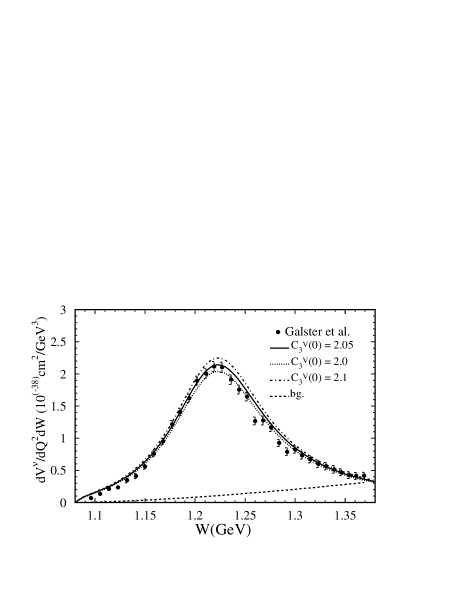
Figure 3: Cross section $dV^{\nu}/{dQ^{2}dW}$ for electroproduction in the $\Delta$ resonance in comparison with Galster et al. data ref15 . The solid, dotted and dot-dashed lines are obtained with $C_{3}^{V}=2.05$, $C_{3}^{V}=2.0$ and $C_{3}^{V}=2.1$, respectively. The dashed line denotes the backgroud contribution.

and then used CVC to obtain the contribution of $V_{\mu}^{+}$ to neutrino induced reactions. We used the formula

$$\frac{dV^{\nu}}{dQ^{2}dW}=\frac{G^{2}}{\pi}\,\,\frac{3}{8}\,\,\frac{Q^{4}}{\pi\alpha^{2}}\,\,\frac{d\sigma^{{\rm em},\,I=1}}{dQ^{2}dW}$$ (8)

to convert the observed ref15 cross sections for the sum of the reactions $e+p\rightarrow e+\left\{\begin{array}[]{c}p\,\pi^{0}\\ n\,\pi^{+}\end{array}\right.$ to the vector contribution in the reaction $\nu+p\rightarrow\mu^{-}+p+\pi^{+}$ denoted in eq. (8) by $V^{\nu}$. The factor $3/8$ originates from the Clebsch-Gordan coefficients relating the matrix elements of the two channels in the electromagnetic case to the matrix element of the weak charged current. We used the data of Galster et al. ref15 at $Q^{2}=0.35\,{\rm GeV}^{2}$ and subtracted the background as suggested by them. Then we converted the points to the vector contribution for the neutrino reaction according to eq. (8). In the same figure we show the neutrino cross section with $C_{3}^{V}(0)=2.05$ (solid), $C_{3}^{V}(0)=2.0$ (dotted), $C_{3}^{V}(0)=2.1$ (dot-dashed) and contribution of background (dashed) and all other form factors equal to zero. Before leaving this topic we mention that the analysis of the electroproduction data ref15 included a contribution from the $D_{13}(1520)$ resonance which was found to be small.

For the axial form factor we use the form given in eq. (7). However, it is advisable to keep an open mind to notice whether a modification will become necessary. With the method described here we have all parameters for the $\Delta$-resonance. We may still change the couplings by a few percent and vary $M_{V}$ and $M_{A}$.

Figure 4: $Q^{2}$-spectrum of the process $\nu p\rightarrow\mu^{-}p\pi^{+}$ in comparison with BNL data ref19 ; furno . The solid curve is with Pauli factor and dotted curve is free case.

There is still the $Q^{2}$ distribution ref18 to be accounted for. The data is from the Brookhaven experiment ref19 ; furno where the experimental group presented a histogram averaged over the neutrino flux and with an unspecified normalization. We used the form factors for the $\Delta$ resonance as introduced above and included the correction from a Pauli factor in the simple Fermi gas model with Fermi momentum $p_{F}=0.16\ {\rm GeV}$ ref10 . The result is the solid curve shown in figure 4 which is satisfactory. For the relative normalization, we normalized the area under the theoretical curve for $Q^{2}\geq 0.2\ {\rm GeV}^{2}$ to the corresponding area under the data. For the other parameters we choose

$$C_{3}^{V}(0)=1.95\, ,\quad C_{5}^{A}(0)=1.2\,,$$ (9)

$$M_{V}=0.84\,{\rm GeV}\, ,\quad M_{A}=1.05\,{\rm GeV}\,.$$

In fact we made a $\chi^{2}$-fit and obtained these values with a $\chi^{2}$ per degree of freedom of 1.76 for the complete $Q^{2}$ region. Furthermore, in order to reduce nuclear effects we performed a fit to all data with $Q^{2}>0.2\ {\rm GeV^{2}}$ and the fit result gave a $\chi^{2}/d.o.f=1.04$. In the theoretical curves we averaged over the neutrino flux for the BNL experiment baker . The dotted curve is the calculation without Pauli factor and the solid one with Pauli suppression factor included which has a small effect. It will be interesting to repeat this analysis when new data become available. From fig. 4 we can see that in the region of small $Q^{2}\lesssim 0.2\ \mathrm{GeV^{2}}$ the theoretical values are significantly above the experimental results which is not cured by a simple Pauli suppression factor which generates small corrections. Clearly, this discrepancy between data and theory is the origin of the worse $\chi^{2}/d.o.f.=1.76$ compared to the result of $\chi^{2}/d.o.f.=1.04$ where the low $Q^{2}$ region has been excluded.

Figure 5: Ratio of total cross sections for RES and QE in comparison with BNL data ref19 . The solid, dotted, and dashed lines have been obtained with $C_{5}^{A}=1.08$, $C_{5}^{A}=1.04$, and $C_{5}^{A}=1.12$, respectively.

Figure 6: Ratio of $Q^{2}$ distributions for RES and QE in comparison with BNL data ref19 . The lines are the same as in fig. 5.

For the resolution of this problem it is reasonable to take the ratio of single pion production (RES) and quasi elastic scattering (QE) events, $\frac{\sigma({\rm RES})}{\sigma({\rm QE})}$. In figs. 5 and 6 we show this ratio for total cross sections and $Q^{2}$ distributions, respectively. The curves have been calculated with $M_{A}=1.05\ {\rm GeV}$ and various values for $C_{5}^{A}(0)$ and have been compared with BNL data ref19 . Since the ratio will reduce flux and experimental uncertainties it is an especially good test for a theoretical model. As can be seen from these figures we find very good agreement between our theoretical curves and the data, particularly also at low $Q^{2}\lesssim 0.2\ {\rm GeV}^{2}$, because uncertainties in the low $Q^{2}$ region which are common to both, resonance and quasi-elastic scattering, drop out in the ratios.

Figure 7: The same as in Fig. 4 using for the theoretical curves the PSY FFs ref10 (red, solid and dashed lines) and SvH FFs ref5 (blue, dotted and dot-dashed lines) for various values of the axial mass $M_{A}$.

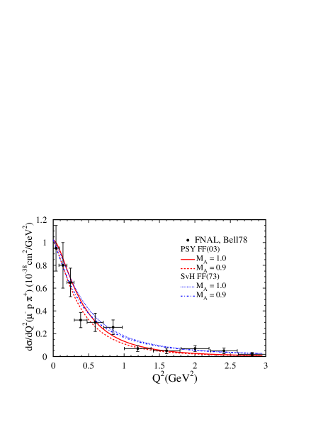
Figure 8: Same as in figure 7 with FNAL data fnal .

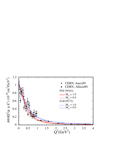
Figure 9: Same as in figure 7 with CERN data cern .

We now turn to a more detailed comparison of our form factors (PSY FFs) ref10 with form factors proposed by Schreiner and von Hippel ref5 (SvH FFs) and additional experimental data for the $Q^{2}$ distribution of single pion production. Figs. 7, 8, and 9 show the flux averaged $Q^{2}$ spectrum for $\Delta$ resonance production in comparison with BNL, FNAL, and CERN data ref19 ; furno ; fnal ; cern . The theoretical curves have been plotted using the PSY form factors (red, solid and dashed lines) and SvH form factors (blue, dotted and dot-dashed lines) for two $M_{A}$ values. All these experimental results have been analyzed with a cut on the invariant mass, $W\leq 1.4\ {\rm GeV}$, such that the $\Delta$ resonance dominates. One can see that the PSY FFs lead to a better description of the data than the SvH FFs for $Q^{2}\gtrsim 1\ \mathrm{GeV^{2}}$. Also notice that the form factors become insensitive to $M_{A}$ for large $Q^{2}$ where $C_{3}^{V}$ (which does not depend on $M_{A}$) is dominant.

IV $\Delta$ resonance electroproduction

In this section we briefly discuss $\Delta$ resonance electroproduction. We start with the fully differential cross section for neutrino reactions ref5 as follows

$$\frac{{\rm d}^{4}\sigma}{{\rm d}Q^{2}{\rm d}W^{2}{\rm d}\Omega_{\pi}^{\star}} = \frac{1}{\sqrt{4\pi}}\frac{{\rm d}^{4}\sigma}{{\rm d}Q^{2}{\rm d}W^{2}}\Big{(}Y_{0}^{0}$$ (10)

$$-\frac{2}{\sqrt{5}}(\widetilde{\rho}_{(33)}-\frac{1}{2})Y_{2}^{0}+\frac{4}{\sqrt{10}}\widetilde{\rho}_{(31)}{\rm Re}Y_{2}^{1}$$

$$-\frac{4}{\sqrt{10}}\widetilde{\rho}_{(3\ -1)}{\rm Re}Y_{2}^{2}\Big{)}$$

with the double differential cross section $\frac{{\rm d}^{4}\sigma}{{\rm d}Q^{2}{\rm d}W^{2}}=N\sum_{i=1}^{3}K_{i}\widetilde{W}_{i}$ given in eq. (1), $\widetilde{\rho}_{(33)},\ \widetilde{\rho}_{(31)},\ \widetilde{\rho}_{(3\ -1)}$ spin density matrix elements and $Y_{l}^{m}(\theta_{\pi},\ \phi_{\pi})$ spherical harmonic functions. This cross section can be easily converted to the electroproduction case by dropping axial vector parts and an appropriate change of the normalization factor. After some algebra we arrive at the following expression for the electroproduction which has a part proportional to $\cos 2\phi_{\pi}^{\star}$ and $\cos\phi_{\pi}^{\star}$ and a part independent of $\phi_{\pi}^{\star}$

$$\frac{{\rm d}^{4}\sigma}{{\rm d}Q^{2}{\rm d}W^{2}{\rm d}\Omega_{\pi}^{\star}} = \frac{N}{\sqrt{4\pi}}\Big{(}\sum_{i=1}^{3}K_{i}\big{(}\widetilde{W}_{i}-D_{i}\frac{(3\cos^{2}\theta_{\pi}^{\star}-1)}{2}\big{)}$$ (11)

$$- 2\sqrt{3}\sin\theta_{\pi}^{\star}\cos\theta_{\pi}^{\star}\cos\phi_{\pi}^{\star}(K_{4}D_{4}+K_{5}D_{5})$$

$$- \sqrt{3}\sin^{2}\theta_{\pi}^{\star}\cos 2\phi_{\pi}^{\star}(K_{6}D_{6})\Big{)}$$

with the normalization factor $N=\frac{\pi\alpha^{2}}{2M^{2}Q^{2}}$, $\theta_{\pi}^{\star}$, and $\phi_{\pi}^{\star}$ the pion polar and azimuthal angles, respectively. The kinematic factors $K_{i},\ i=1,...,6$ and the structure functions $\widetilde{W}_{i},D_{i}$ can be found in ref5 and depend on the vector form factors introduced in Sec. II.

Figure 10: Electroproduction data electro for the reaction $e+p\rightarrow e+p+\pi^{0}$.

Figure 11: The same as in fig. 10 for small $Q^{2}$ data siddle .

For our numerical comparison with electroproduction data we have calculated the fully differential cross section in eq. (11) using the vector form factors given in eqs. (4) and (5). In fig. 10 we show electroproduction data electro for the reaction $e+p\rightarrow e+p+\pi^{0}$ in dependence of the pion polar angle $\theta_{\pi}$ for various pion azimuthal angles $\phi_{\pi}$ for fixed $Q^{2}=2.8\ {\rm GeV}^{2}$, $W=1.235\ {\rm GeV}$ and electron energy $E_{e}=3.2\ {\rm GeV}$. Similarly, in fig. 11 experimental results at small momentum transfers $Q^{2}=0.45\ \mathrm{GeV^{2}}$ and $Q^{2}=0.75\ \mathrm{GeV^{2}}$ are shown. As can be seen the description of the data by our simple model is already quite reasonable with exception of data points at $|\phi_{\pi}|\geq 135^{\circ}$ in the upper panels in fig. 10. It should be noted that the theoretical curves have been obtained without fine tuning of the parameter $C_{3}^{V}(0)$, for which we took the value $C_{3}^{V}(0)=2.0$, and without including the background from the $I=1/2$ channel and a non-resonant background which is expected to be of the order of $10\%$. A more detailed comparison will be presented elsewhere winp .

V Conclusions

Single pion neutrino production at low energies is important to measure properties of neutrino oscillations. There exist already more complicated calculations, i.e., with more parameters and a more complicated functional form of the form factors. On the other hand, our approach is particularly simple and self-contained. Therefore it is helpful for the physical interpretation.

We have analyzed the differential cross section $\frac{{\rm d}\sigma}{{\rm d}Q^{2}}$ in terms of two form factors which are described by two free parameters $M_{A}$ and $M_{V}$ and compared our results with several experimental data. We obtained a good fit to BNL data furno with a $\chi^{2}/d.o.f=1.04$ for $Q^{2}\geq 0.2\ {\rm GeV}^{2}$. However, for $Q^{2}\leq 0.2\ {\rm GeV}^{2}$ the theory value is too high. A possible explanation are medium effects which are not properly taken into account. The Pauli suppression factor has a small effect which does not resolve the discrepancy. To shed light on this problem we took the ratio $\frac{\sigma{\rm(RES)}}{\sigma{\rm(QE)}}$ and found very good agreement with BNL data furno .

From these comparisons we conclude that the neutrino production of the $\Delta$ resonance can be described by two form factors $C_{3}^{V}$ and $C_{5}^{A}$. $C_{3}^{V}$ is consistent with electroproduction data and $C_{5}^{A}$ can be determined only from neutrino data.

We verified the consistency of our model by comparing with further existing neutrino production data. Moreover, we found that our form factors gave a better description than the form factors originally proposed by Schreiner and von Hippel ref5 .

Finally, we performed a first comparison with more differential electroproduction data and found reasonable agreement also here. In this comparison we have neglected the background from the isospin $I=1/2$ channel and a non resonant background which is of the order of $10\%$ at $W=1232\ \mathrm{GeV}$.

In the future we will include higher resonances and non-resonant background and perform a more detailed comparison with electroproduction data in order to study further the connection between neutrino- and electroproduction.

References

- (1) C.H. Albright and L.S. Liu, Phys. Rev. 140 (1965) 748.
- (2) S.L. Adler, Ann. of Physics 50 (1968) 189.
- (3) P. Zucker, Phys. Rev. D4 (1971) 3350.
- (4) C.H. Llewellyn Smith, Phys. Rep. 3 (1972) 261.
- (5) P.A. Schreiner and F. von Hippel, Nucl. Phys. B58 (1973) 333.
- (6) G. L. Fogli and G. Nardulli, Nucl. Phys. B160 (1979) 116.
- (7) G. L. Fogli and G. Nardulli, Nucl. Phys. B165 (1980) 162.
- (8) D. Rein and L. Sehgal, Ann. Phys. 133 (1981) 79.
- (9) S. K. Singh, M. T. Vicente Vacas and E. Oset, Phys. Lett. B416 (1998) 23.
- (10) E.A. Paschos, M. Sakuda and J.Y. Yu Phys. Rev. D69 (2004) 014013.
-
(11)
E.A. Paschos, L. Pasquali and J.Y. Yu,
Nucl. Phys. B588 (2000) 263;
E.A. Paschos and J.Y. Yu, Phys. Rev. D65 (2002) 033002;
I. Schienbein and J.Y. Yu, Proceedings of the 2nd International Workshop on Neutrino-Nucleon Interactions (NUINT02), hep-ph/0308010; E.A. Paschos, D.P. Roy, I. Schienbein and J.Y. Yu, Phys. Lett. B574 (2003) 232; Proceedings of the 2nd International Conference on Flavor Physics 2003 (ICFP2003), Korea, Seoul, October 2003, hep-ph/0312123. - (12) S. Fubini, Y, Nambu and V. Wataghin, Phys. Rev. 111 (1958) 329.
- (13) R. H. Dalitz and D. G. Sutherland Phys. Rev. 146 (1966) 1180.
-
(14)
W. Bartel et al.
Phys. Lett. B28 (1968) 148;
S. Galster et al., Phys. Rev. D5 (1972) 519;
W. Bartel et al., Phys. Lett. B35 (1971) 181. - (15) A.J. Dufner and Y.S. Tsai, Phys. Rev. 168 (1968) 1801.
- (16) L. Tiator et al., Eur. Phys. J. A17 (2003) 357; S. Kamalov et al., Phys. Rev. C64 (2001) 032201.
- (17) T. Sato and T.-S. H. Lee, Phys. Rev. C63 (2001) 055201.
- (18) G. Olsson et al., Phys. Rev. D17 (1978) 2938.
- (19) M. Sakuda in: NUINT 01 Conference, Proc. Suppl. Nucl. Phys. 112 (2002) 109, and E.A. Paschos, ibid. page 89.
- (20) T. Kitagaki et al., Phys. Rev. D34 (1986) 2554.
- (21) K. Furuno, Talk at the 2nd Int. Conf. NUINT 02, Irvine, CA (Dec. 2002).
- (22) N.J. Baker, et al., Phys. Rev. D23 (1981) 2499.
- (23) J. Bell, et al., Phys. Rev. Lett. 41 (1978) 1008.
-
(24)
G.T. Jones,
Z. Phys. C43 (1989) 525;
D. Allasia et al., Nucl. Phys. B343 (1990) 285. - (25) V.V. Frolov et al, Phys. Rev. Lett. 82 (1995) 45.
-
(26)
R. Siddle et al.,
Nucl. Phys. B35 (1971) 93;
J. C. Adler et al., Nucl. Phys. B46 (1972) 573. - (27) E.A. Paschos, M. Sakuda, I. Schienbein and J.Y. Yu, work in progress.