Multi-Module Modeling of Heavy Ion Reactions
and the 3rd Flow Component^†

Abstract

Fluid dynamical calculations with QGP showed a softening of the directed flow while with hadronic matter this effect is absent. On the other hand, we indicated that a third flow component shows up in the reaction plane as an enhanced emission, which is orthogonal to the directed flow. This is not shadowed by the deflected projectile and target, and shows up at measurable rapidities, $y_{c}m=1-2$. To study the formation of this effect initial stages of relativistic heavy ion collisions are studied. An effective string rope model is presented for heavy ion collisions at RHIC energies. Our model takes into account baryon recoil for both target and projectile, arising from the acceleration of partons in an effective field. The typical field strength (string tension) for RHIC energies is about 5-12 GeV/fm, what allows us to talk about ”string ropes”. The results show that QGP forms a tilted disk, such that the direction of the largest pressure gradient stays in the reaction plane, but deviates from both the beam and the usual transverse flow directions. The produced initial state can be used as an initial condition for further hydrodynamical calculations. Such initial conditions lead to the creation of third flow component. Recent $v_{1}$ measurements are promising that this effect can be used as a diagnostic tool of the QGP. Collective flow is sensitive to the early stages of system evolution. To study the sensitivity of the flow signal, we have calculated flow harmonics from a Blast Wave model, a tilted, ellipsoidally expanding source. We studied recent experimental techniques used for calculation of the $v_{n}$ Fourier coefficients and pointed out a few possible problems connected to these techniques, which may impair the sensitivity of flow analysis.

1 Introduction

In high energy heavy ion reactions many thousand particles are produced in the reaction, so, we have all reasons to assume that in a good part of the reaction the conditions of the local equilibrium and continuum like behavior are satisfied. The initial and final stages are, on the other hand, obviously not in statistically equilibrated states, and must be described separately, in other theoretical approaches. The different approaches, as they describe different space-time (ST) domains and the corresponding approaches can be matched to each other across ST hyper-surfaces or across some transitional layers or fronts. The choice of realistic models at each stage of the collision, as well as the correct coupling of the different stages or calculational modules are vital for a reliable reaction model.

The fluid dynamical (FD) model plays a special role among the numerous reaction models, because it can be applied only if the matter reaches local thermal equilibrium. If this happens the matter can be characterized by an Equation of State (EoS). This is what we are actually looking for in these experiments and this is why fluid dynamics is so special.

2 Measurement of Colective Flow

In relativistic heavy ion collisions collective flow was predicted to occur already in the early 1970s SMG (1974); CJT (1973) and proved to exist beyond doubt in 1984 first by the Plastic Ball collaboration at LBL PB8 (1984). Then, using the method worked out by Danielewicz and Odyniecz based on the physical properties of heavy ion collisions DO8 (1985), the directed collective flow was possible to detect in smaller samples and in a wide range of detectors.

A variety of collective flow patterns were detected, the “squeeze out”, the “elliptic flow”, the “anti flow” or “3rd flow component”, etc. Anisotropic flow is defined as azimuthal asymmetry in particle distributions with respect to the reaction plane, spanned by the beam direction and the impact parameter vector. The increasing complexity of flow patterns naturally led to attempts to classify the flow patterns in a more systematic way, on principal ground, and not just following the new experimental observations.

A formal classification of the azimuthal asymmetries was recently introduced via the coefficients, $v_{n}$, of the Fourier expansion of the azimuthal distribution of particles PV9 (1998):

$$E\frac{d^{3}N}{d^{3}P}=\frac{1}{2\pi}\frac{d^{2}N}{p_{t}dp_{t}dy}\left(1+2\sum_{n}v_{n}\cos{(n\,\Phi)}\right)\ ,$$ (1)

where $\Phi$ is the azimuth angle with respect to the true reaction plane of the event. In experiments anisotropic transverse flow manifests itself in the distribution of $\phi=\Phi+\Psi_{R}$, where $\phi$ is the measured azimuth for a track in detector coordinates, and $\Psi_{R}$ is the azimuth of the reaction plane in the event, which varies event by event in the coordinate frame of the detector. Using this definition the coefficients have a transparent meaning:

$$v_{n}=\langle\cos(n(\phi-\Psi_{R}))\rangle$$

so that the directed flow is $v_{1}=\langle p_{x}/p_{t}\rangle$ and the elliptic flow is $v_{2}=\langle(p_{x}/p_{t})^{2}-(p_{y}/p_{t})^{2}\rangle$ , where the average is taken over all emitted particles (in a given rapidity, $y$, and transverse momentum $p_{t}$ bin), in all events. $\Psi_{R}$ can not be directly measured, and randomly takes any value in $[0,2\pi]$ due to the random direction of the impact parameter vector of the event.

Anisotropic flow has been fully recognized as an important observable providing information on the early stages of heavy ion collisions Sor (1997); ZGY (1999); Ol9 (1992). The development of flow is closely related to the pressure gradients, and thus, to the equation of state of the nuclear matter formed in the collision RR9 (1997); Shu (1999). Collective flow is also believed to be a promising signal to detect the creation of the quark-gluon plasma LaD (1999); Bra (2000); BS0 (2002). An increased attention to collective flow has also resulted in significant improvements in the techniques and methods of analysis and presentation of the experimental data. PHENIX, PHOBOS and STAR experiments at RHIC produced a wealth of information on the flow components STA (2001, 2002, 2003, 2004); PHO (2002, 2003); PHE (2002, 2003).

3 The Soft Point

The most straightforward and first observed collective flow phenomenon was the directed transverse flow. The projectile and target in the collision have overlapped, the participant region is compressed and heated up, which results in high pressure, $P$. The spectator regions, which are not compressed and heated up so much have contact with the hot central zone. The size of the contact surface, $S$, is of the order of the cross-section of the nuclei or somewhat less, depending on the impact parameter. During the collision the spectators and participants were in contact for a period of time $\tau$ and in this time the spectators acquired a directed transverse momentum component of

$$p_{x}\approx P\times S\times\tau$$

At a few hundred MeV/nucleon Beam energy the directed transverse flow momentum was almost as large as the random average transverse momentum and it was also close to the CM beam momentum.boo (1994)

The effect was dominant, it was used to estimate the compressibility of nuclear matter, and the general expectation was that this is a good tool to find the threshold of the phase transition of the Quark Gluon Plasma. The reason is that the pressure decreases considerably versus the energy density in a first order phase transition, when the phase balance and formation of the new phase prevents the pressure from increasing in the mixed phase region. All estimates indicated that this is a strong and observable decrease in the pressure, and it has got the name the ”soft point”.

To some extent the expectations were fulfilled, the directed transverse flow decreased as the beam energy was increased above 1 GeV and further. This was obvious compared to the beam momentum, but the decrease was also well observable compared to the average transverse momentum.

The reason is actually simple: although at high energies the pressure should increase the target and projectile are becoming more and more Lorentz contracted, and the overlap time also. So, the directed transverse momentum the non-participant matter could acquire was

$$p_{x}\approx P\times\frac{S}{\gamma}\times\frac{\tau}{\gamma}\ .$$

Thus, at high energies the directed flow could not compete with the trivial effect of reducing the flow by $\gamma^{2}$. This eliminated the interest in the directed flow, while the elliptic flow became a dominant and strong effect.

4 The Initial State

The elliptic flow, which is observable in the coefficient of the 2nd harmonic, $v_{2}$, PV9 (1998) of the flow analysis, was not effected by the increasing beam energy because it developed in the CM frame in the participant matter, due to a special symmetry in the initial state and due to the large pressure gradient in the direction of the reaction plane. The elliptic flow took over the role of the directed flow, and became an important tool in determining the basic reaction mechanism. Only models, which included a large collective pressure could reproduce the data, i.e. mainly fluid dynamical models. On the other hand, the elliptic flow effect was so strong that most fluid dynamical models could fit the data, even rather simple, one- and two- dimensional ones, so it was not a very strong diagnostic tool.

A deeper insight into fluid dynamical calculations indicated that a similar effect, arising exclusively from participant matter, should be possible to see also in the $v_{1}$ harmonic. This was first observed in 1999 LaD (1999) based on earlier FD calculations, which included a QGP EoS. The effect was named the 3rd flow component.

The effect was verified at the CERN SPS, but it was initially not detected at RHIC. Now at the beginning of this year, first STAR then two other collaborations have succeeded to measure the $v_{1}$ harmonic coefficient of the collective flow at RHIC also. STA (2004); Old (2004) This indicated to us that one needs extended theoretical studies, to map the sensitivity of this measurable.

As all fluid dynamical effects it depends on the initial state and on the EoS. It is of special interest how this effect depends on the initial state because this may shed light on the mechanisms of the formation of QGP in heavy ion reactions.

The initial state models in our recent works are based on a collective (or coherent) Yang-Mills model, a versions of flux-tube models. This approach GC8 (1986) was implemented in a Fire-Streak geometry streak by streak and it was upgraded to satisfy energy, momentum and baryon charge conservations exactly at given finite energies MCS (2001a, 2002). The effective string-tension was different for each streak, stretching in the beam direction, so that central streaks with more color (and baryon) charges at their two ends, had bigger string-tension and expanded less, than peripheral streaks. The expansion of the streaks was assumed to last until the expansion has stopped. Yo-yo motion, as known from the Lund-model was not assumed.

Our calculations show that a tilted initial state is formed, which leads to the creation of the third flow component LaD (1999), peaking at rapidities $|y|\approx\pm 0.75$ MCS (2001b). Recent, STAR $v_{1}$ data STA (2004) indicate that our assumption that the string expansion lasts until full stopping of each streak, may also be too simple and local equilibration may be achieved earlier, i.e. before the full uniform stopping of a streak. We did not explicitly calculate dissipative processes, some friction within and among the expanding streaks is certainly present and experiments seem to indicate that this friction is stronger. The expanding strings are shown in Fig. 1

With time the streaks expand and move to the right and left on the top and bottom respectively. This motion will be reflected in the subsequent FD motion also so the tilted transverse expansion will be observed at large polar angles, i.e. relatively low rapidities. The position of the 3rd component flow peaks depends on the (i) impact parameter, (ii) the effective time of the left/right longitudinal motion, (iii) the string tension determining the lengths of the streaks, (iv) the thickness of the configuration which determines the initial pressure gradient. The string tension varies as a function of the distance of a given streak from the central beam axis, because of the amount of the matter at the ends of the streaks. This determined the amount of color charge, and so the string tension is

$$\sigma=A\left(\frac{E_{cm}}{m}\right)\frac{\sqrt{N_{1}N_{2}}}{\delta x\ \delta y}$$

given in terms of the Baryon charges at the two ends of the streak, $N_{1}$ and $N_{2}$, and the cross section of the string, $\delta x\ \delta y$.

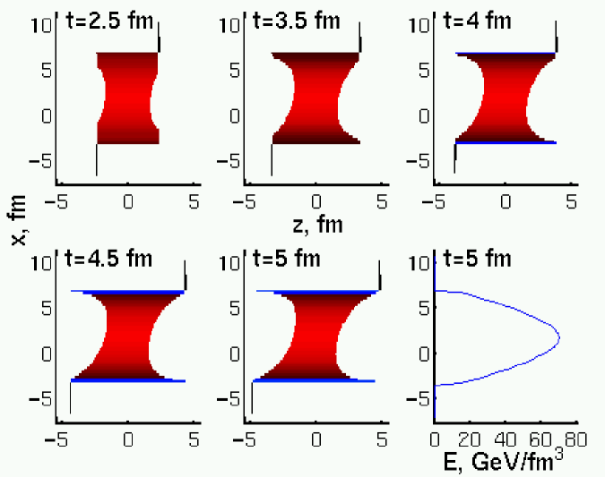
Figure 1: Au + Au collision at $E_{cm}=65+65$ GeV/nucl, $b=0.25\times 2R_{Au}$, and the parameter determining the string tension $A=0.08$, $E=T_{00}$ is presented in the reaction plane as a function of $x$ and $z$ for different times in the laboratory frame. The final shape of the QGP volume is a tilted disk $\approx 45^{0}$, and the direction of the fastest expansion will deviate from both the beam axis and the usual transverse flow direction, and will generate the third flow component. Note that the streaks are moving in the CM frame. From MCS (2002)

Although, there are several effects determining the angle of the 3rd flow component, some of these can be traced down by other measurements also: the impact parameter by the multiplicity, the effective expansion time and size by two particle correlation measurements, etc. Thus, there is a reasonable possibility that the $v_{1}$ measurements will lead to a more detailed insight to the details of the QGP formation in heavy ion reactions.

The subsequent fluid dynamical calculations show the development of the 3rd flow component from these type of initial states. These FD model calculations have to be supplemented with a Freeze Out model. There is a very essential development in this field also, and we can have different levels of approach from simplified freeze out descriptions across an FO hypersurface using an improved Cooper-Fry description, or a full kinetic description, originating from a modified Boltzmann Transport Equation approach. This final step is complicated further by the fact that the data indicate a rapid and simultaneous hadronization and freeze out.

Nevertheless, we expect that the $v_{1}$ flow data will be sufficiently detailed and accurate soon, and the 3rd flow component will be an effect which is sufficiently strong that the complex final effects at the freeze out will allow a successful analysis of the matter properties via these flow measurements.

5 Analysis of flow components in experiments

There are several techniques, which have been used to calculate flow components. One of the most important, however, far not trivial task is the identification of the reaction plane. The Danielewicz-Odyniecz method DO8 (1985) constructed an estimated event plane $\Psi_{\{EP\}}$, using the the momentum vectors of all detected particles, introducing a rapidity dependent weighting (where the sign of the CM rapidity was crucial), and by eliminating self correlations. This weighting in principle should also be used in the Fourier expansion method PV9 (1998), especially for odd harmonics. When the Fourier expansion method is used, each measurable harmonic can yield an independent estimated $\Psi_{n}$, event plane of the $n$th harmonic. These estimated reaction planes may differ from one-another, which is clearly incorrect, as there is only one reaction plane in one event. In some of the recent techniques the reaction plane is not evaluated explicitly, because the Fourier coefficients, $v_{1}$, $v_{2}$, $v_{3}$, … can be obtained without. We will show that these methods may lead to problems as well.

5.1 Techniques for analyzing $v_{n}$

In this section we will briefly discuss three of the experimental methods of flow analysis.

The flow coefficients can be obtained by the pairwise correlation WAN (1991) of all particles without referring to the reaction plane. This two-particle correlation method produces the squares of the coefficients:

$$v_{n}^{2}=\langle\cos{[n(\phi_{i}-\phi_{j})]}\rangle_{i\neq j}\ .$$

The method has the advantage that the reaction plane does not need to be determined or estimated by an event plane.

In the event plane method PV9 (1998) one investigates the correlation of particles with an event plane, which is an estimation to the real reaction plane. The flow components are given by:

$$v_{n}^{obs}=\langle\cos{[n(\phi_{i}-\Psi_{n})]}\rangle\ ,$$

where $\Psi_{n}$ is the observed event plane of order $n$. The observed event plane is not the true reaction plane, therefore, the observed coefficients, $v_{n}^{obs}$, have to be corrected by dividing by the resolution of the event plane. The resolution is estimated by measuring the correlations of the event planes of sub-events. For details consult PV9 (1998) or PHO (2002).

The sub-event method is used originally in the Danielevicz-Odyniecz method DO8 (1985) to determine the accuracy of the estimated reaction plane from the data. Using it in the Fourier expansion method, there are several ways to choose sub-events. Most trivially one can divide each event randomly into two sub-events. The partition using two (pseudo) rapidity regions (better separated by $\Delta y>0.1$) could greatly suppress the contribution from quantum statistics effects and Coulomb (final state) interactions STA (2002), as well as could also be used to correctly identify the first harmonic reaction plane, $\Psi_{1}$.

Recently, a multiparticle correlation or cumulant method BOR (2001, 2002) is widely used. This method has larger statistical errors than the two-particle analysis. The most recent STAR data on the directed flow STA (2004) were calculated with three-particle cumulants combined with the event plane method.

5.2 Recent detection techniques

In experimental techniques using the Fourier expansion method, each measurable harmonic can yield an independent, estimated $\Psi_{n}$, via the event flow vector $Q_{n}$ with the definition STA (2002):

$$Q_{n}\ \cos(n\Psi_{n})=\Sigma_{i}\cos(n\phi_{i}),\ \ \ Q_{n}\ \sin(n\Psi_{n})=\Sigma_{i}\sin(n\phi_{i})\ ,$$

where the sums extend over all particles in a given event.

First of all these estimated reaction planes may be different from one-another, furthermore as the summation goes over the whole acceptance of the detector, which is symmetric in rapidity, $y$ STA (2002) without weighting by rapidity, the first harmonic, $v_{n}$, is eliminated by construction, because it involves a Forward/Backward azimuthal antisymmetry, and so, the Forward and Backward contributions cancel each other in the above definition.

One might argue that such a Forward/Backward azimuthal anti-correlation is a consequence of momentum conservation, thus, it is a non-flow correlation, but fluid dynamics is nothing else then the collective form of energy and momentum conservation!

More precisely, in the infinite particle number limit, fluid dynamics really leads to a single particle momentum distribution after integrating the contributions of all fluid elements. This is a consequence of the assumption of local local equilibrium, a fundamental assumption in fluid dynamics, and of the assumption of molecular chaos. When we consider finite multiplicities and smaller samples, correlations may arise from global momentum conservation. To subtract these correlations as non-flow effects is questionable. Furthermore, fluid dynamics must be supplemented by some Freeze Out (FO) prescription to obtain measurables.

Due to the Freeze Out process, the local thermal equilibrium ceases to exist, the post FO distribution must be an out of equilibrium, non-thermal distribution. In the FO process the assumption of molecular chaos does not hold, so the FO process leads to correlations. There is a third effect, inherent in fluid dynamical descriptions when sudden and rapid hadronization coincides with freeze out. This can be described in a non-thermal string fragmentation, coalescence or recombination picture, which lead to correlations also. The above mentioned three effects fundamentally influence the measured flow patterns, and the measured Fourier harmonics, so it is highly questionable if these should be excluded from the determination of the reaction plane, as it is done in the cumulant expansion method.

For the higher odd harmonics, the determination of reaction plane can be similarly problematic, as these appear dominantly in asymmetric, $A+B$, collisions, and then the beam direction is crucial, and the method eliminates this important physical information. Thus, the elimination of the information provided by the longitudinal motion of emitted particles and the longitudinal symmetries and asymmetries severely impair the analysis of the collective flow.

In case of even harmonics exclusively, the weighting does not seem to be too important and one may conclude (wrongly) that it can be omitted without severe consequences. For even harmonics, however, there is a symmetry for positive and negative $x$-values, and so, the Projectile/Target directions cannot be identified, i.e. only the reaction plane is identified but not the direction of the impact parameter vector ${\mathbf{b}}$. If this estimated reaction plane is used for the evaluation of the coefficients, $v_{n}$, the Target and Projectile directions may appear randomized in the sample. If weighting is used, but it is Forward/Backward symmetric, e.g. $w_{i}(y)=v_{2}(y)$ STA (2002), this does not solve the problem discussed here. As a consequence Forward/Backward azimuthal asymmetries, will be decreased or eliminated by this misidentification, and these will contribute and enhance the measured coefficients of even harmonics, e.g. the elliptic flow.

The above mentioned situation may occur even if the reaction plane determination is implicit and not discussed at all. Due to complicated experimental setups, the event plane determination varies to a large extent, and different methods can even be mixed with each other. In these cases it is very difficult to judge the accuracy and precision of event plane determination. An example is, the evaluation of $v_{1}$ by the STAR collaboration, where two different methods determining the reaction plane yield different coefficients STA (2004); Old (2004) $v_{1}=(-0.25\pm 0.27(stat))\%y$ vs. $v_{1}=(-0.5\pm 0.5(stat))\%y$, which agree within error and are even consistent with zero within error.

6 Calculation of flow components

We have calculated the directed and elliptic flow from a tilted, ellipsoidally expanding particle emitting source. Our tool is a simple, blast wave type hydrodynamic model. The tilt angle, $\Theta$, represents the rotation of the major (longitudinal) direction of expansion from the direction of the beam. In the presented calculations $\Theta=\pm 5.7^{\circ}$. We have divided our fireball into cubic cells by a grid in x, y, z coordinates, as it is done in most hydrodynamic models. The aim of the introduced discretization was to produce similar output as other models have, which makes it possible to change the presently used simple blast wave model to more sophisticated ones without further changes in the next steps of the calculation.

Also, the FO layer is discretized on this grid. Due to this discretization, the “fluid-cells” do not match the spherical layer exactly, the volume of the cells, and so all conserved quantities have some discretization error. This depends on the choice of radius, layer thickness, cell size and the way which cells are selected to be in the layer. However, one can vary these parameters, to achieve a small relative error in the normalization. The present example yields a relative error below $1\%$ which is already much smaller than the statistical errors of the experimental techniques.

6.1 Theoretical background

The contribution of a fluid cell to the final baryon Phase-Space (PS) distribution is:

$$\frac{dN_{c}}{d^{3}p}=\gamma\,V_{c}\,\>\frac{p^{\mu}\,d\sigma_{\mu}}{p^{0}}\ \ f_{F.O.}(x,\,p)\ ,$$ (2)

where $\gamma\,V_{c}$ is the proper volume of one fluid cell, $f_{F.O.}(x,\,p)$ is the freeze out distribution and $d\sigma_{\mu}$ is the normal of the FO surface. Using the relations $p=(p^{0},p_{\parallel},{\mathbf{p}_{\perp}})$, $p_{\parallel}=p^{0}\ dy$ and $p_{t}=|{\mathbf{p}_{\perp}}|$, we can get the azimuthal distribution per unit rapidity as

$$\frac{dN_{c}}{dy\ d\phi}=\int\frac{d^{3}p}{dy\ d\phi}\ \frac{dN_{c}}{d^{3}p}=\gamma\,V_{c}\,\int\frac{d^{3}p}{dy\ d\phi}\ \frac{p^{\mu}\,d\sigma_{\mu}}{p^{0}}\ f_{F.O.}(x,\,p)=$$

$$=\gamma\,V_{c}\,\int dp_{t}\ p_{t}\ \ (p^{\mu}\,d\sigma_{\mu})\ f_{F.O.}(x,p)\equiv\ \int dp_{t}\ p_{t}\ G_{c}(p_{t},\phi_{CM},y)\ .$$ (3)

When we evaluate the azimuthal asymmetry this is done with respect to the reaction plane. The $\phi_{CM}$ is the azimuth-angle of particles in the C.M. frame where these are measured. Then, the coefficients of the different harmonics, $v_{1}$, $v_{2}$, etc. can be evaluated via additional numerical integrations over $\phi_{CM}$ azimuth angle.

Thus,

$$v_{n}(y)=\frac{\displaystyle{{\sum_{c}\int\cos{(n\phi_{CM})}\,\gamma\,V_{c}\,(p^{\mu}\,d\sigma_{\mu})\ f_{F.O.}(x,p)d^{2}p_{t}}}}{\displaystyle{\sum_{c}\ dN_{c}/dy}}\ .$$ (4)

For the FO surface we may assume that the local momentum distribution is a Jüttner distribution:

$$f_{F.O.}(x,\,p)=f^{J\ddot{u}ttner}(p)\equiv\frac{g_{n}}{(2\pi\hbar)^{3}}exp\left(\frac{\mu-p^{\mu}u_{\mu}}{T}\right)\ .$$

In this case Eq. (4) takes the form

$$v_{n}(y)=\frac{\displaystyle{\sum_{c}\,K\,\gamma V_{c}\ \int dp_{t}\ p_{t}\ d\phi_{CM}\,\cos{(n\,\phi_{CM})}g_{c}(p_{t},\phi_{CM},y)}}{\displaystyle{\sum_{c}\ dN_{c}/dy}}$$

where we have introduced the following notations:

$$g_{c}(p_{t},\phi_{CM},y)\equiv\left[H\,\sqrt{m^{2}+p_{\bot}^{2}}-\,{\rm\bf{p}_{\bot}}\,\gamma_{\sigma}\>{{\rm\bf d\sigma}_{\bot}}\>\right]\cdot e^{-h\,\sqrt{m^{2}+p_{\bot}^{2}}+\,{\rm\bf{p}_{\bot}}\,{\rm\bf g}}\ ,$$

$$H\equiv\gamma_{\sigma}(\cosh y-d\sigma_{\parallel}\,\sinh y)\ ,\quad h\equiv\gamma(\cosh y-v_{\parallel}\,\sinh y)/T\ ,\quad{\rm\bf g}\equiv\gamma\>{\rm\bf v_{\bot}}/T\ ,$$

$$K\equiv(g_{n}\cdot e^{\,\mu/\,T})/(2\pi\hbar)^{3}=(g_{n}\cdot n)/(4\pi\,m^{2}\,T\,K_{2}(m/T))\ .$$

To calculate the $v_{n}$ harmonics one has to perform double integrals. The calculation of the numerator can only be done numerically. However, the denominator, which is actually the rapidity distribution of particles, $dN/dy$, has an analytical solution. The solution for the case of $d\sigma^{\mu}=u^{\mu}$ was derived and shown in boo (1994) in Eq. (7.6). For the more realistic, general case, when $d\sigma^{\mu}\not=u^{\mu}$ such analytical result, according to our knowledge, has not yet been shown in the literature. We have, however, found such solution in this latter case as well, NyH (2004) and derived a relatively simple formula to calculate the rapidity distribution, i.e. the denominator of the $v_{n}$ flow components:

$$\frac{dN_{c}}{dy} = 2\pi\,K\,\gamma V_{c}\,\gamma\prime^{3}\,\frac{H}{h}m^{2}\,\left(1-\frac{g\,G}{h\,H}\right)\left[\frac{2\,\gamma\prime^{2}}{h^{2}\,m^{2}}+\frac{2\,\gamma\prime}{h\,m}+1\right]e^{-\frac{h}{\gamma\prime}m}\ .$$ (5)

¿From Eq. (5) the final rapidity distribution can be calculated by summing over all fluid cells, i.e. $dN/dy=\sum_{c}dN_{c}/dy$. The new formula makes further calculations faster, because we can reduce the number of time consuming numerical integrations.

6.2 Results for directed and elliptic flow

Our primary aim is to show why the identification of the reaction plane is so important, and how the odd harmonics may be eliminated by construction using the cumulant method without proper weighting. As we have mentioned in Sec. 5.2, the acceptance of the detector is symmetric in rapidity STA (2002). Odd harmonics involve a Forward/Backward azimuthal antisymmetry, therefore, without weighting by rapidity taking into account the sign of it, i.e. whether the detected particle came from the target or projectile side, the Forward and Backward contributions may cancel each other. To show this, we have calculated flow components from two tilted ellipsoidally expanding sources, which differ from one-another only in the sign of the tilt angle, i.e. we have changed the projectile and target side. Then we calculated the average of both the directed and elliptic flow components coming from the two opposite tilted sources, which simulates the situation when only the reaction plane is identified, but not the impact parameter, as the projectile and target directions are not known.

Figure 2 shows the elliptic flow, $v_{2}$, result as a function of the transverse momentum, $p_{t}$. These figure is less relevant for our primary aim, but demonstrates that even a simple blast wave model can reproduce some of the main characteristics of the observed data. We have plotted a less wide $p_{t}$ region, because it was shown earlier STA (2003) that elliptic flow at RHIC can be described by hydrodynamical models for $p_{t}$ up to $2GeV/c$. $v_{2}$ rises almost linearly up to $p_{t}=1GeV/c$, then deviates from a linaer rise and starts to saturate.

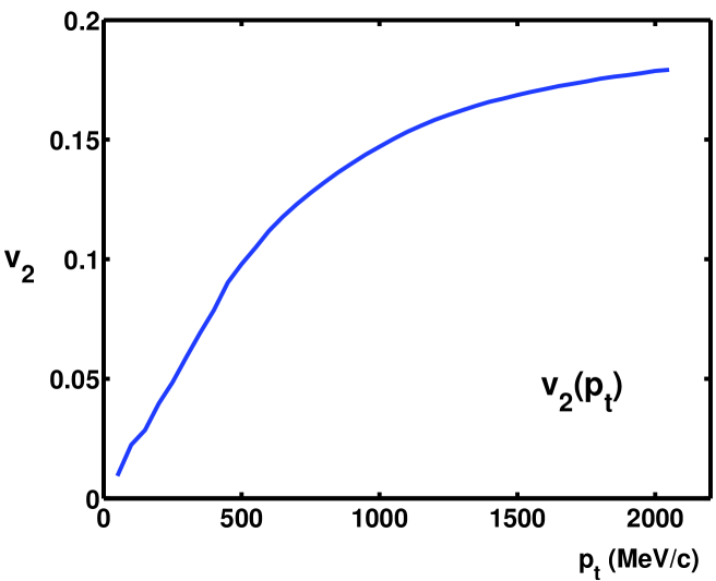
Figure 2: Elliptic flow of nucleons, $v_{2}$, as a function of transverse momentum, $p_{t}$, at mid-rapidity, $y=0$, from NyH (2004). The the velocity is normal to the tilted ellipsoid, with axes $a,b,c=6,8,10fm$. The sudden FO happens with $T=165MeV$ and $n=0.5fm^{-3}$. The result is in good agreement with the experimental data presented in STA (2004).

Figure 3 demonstrates that identification of the Projectile/Target plays a less important role in the determination of the second harmonic, such as higher order even harmonics. For even harmonics there is a symmetry for positive and negative $x$-values, thus the role of introducing weights with opposite signs for positve and negative rapidities in the event plane or cumulant method is not transparent. This may lead to the wrong conclusion that weighting is not important. In Figure 3 we have plotted the elliptic flow , $v_{2}$, as a function of rapidity, $y$. The distribution is too narrow compared to the expected one and to experimental data. However, it is possible to improve the recent result by using more suitable set of parameters. The dashed-dotted curve refers to the case when the tilt angle is positive, $\Theta=5.7^{\circ}$, while the continuos line represents the result from averaging $v_{2}(\Theta=5.7^{\circ})$ and $v_{2}(\Theta=-5.7^{\circ})$, i.e. elliptic flows from two oppositely tilted sources. The two results are nearly identical, therefore one can hardly see that there are indeed two curves in the figure.

Let us perform a similar investigation for the directed flow, or first harmonic, $v_{1}$. We calculate $v_{1}$ as a function of rapidity, $y$, in the case of two oppositely tilted ellipsoidal sources. The dashed-dotted curve refers to the case with $\Theta=5.7^{\circ}$.

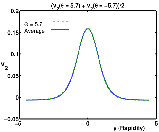
Figure 3: Elliptic flow, $v_{2}$, as a function of rapidity, $y$. The distribution is somewhat narrow. This problem can be avoided by better choice of parameters. One can see that the $v_{2}$ result is not sensitive too the change of projectile and target side, the two curves are almost identical.

One can see, that $v_{1}(y)$ is definitely not constant zero and the so called “wiggle”, which is well known from earlier experiments with lower energies, appears. The situation changes dramatically when we construct the averaged $v_{1}$, which demonstrates what happens when we partly reverse the projectile and target side, i.e. we use the event plane or cumulant method without proper weighting. As the continuos curve shows, in this case $v_{1}$ is in principle set to zero, $v_{1}(y)\approx 0$. As we have mentioned at the beginning of Section 6, we have introduced a discretization of our freeze out layer. This discretization leads to the inaccuracy in our calculations. In other calculations with bigger tilt angles, $|\Theta|>10^{\circ}$ such “waves” were not seen. However, theoretical considerations do not support that the source can be so much tilted at RHIC energies, therefore, we have chosen smaller angles in our presentation.

7 Conclusions

We have studied the importance of the initial state in the development of cllective flow in heavy ion collisions. The directed transverse flow weakens at increasingly ultra-relativistic energies, so that its recovery after the soft point cannot be expected or easily demonstrated.

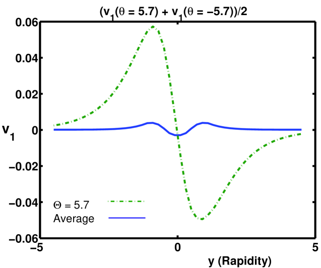
Figure 4: Directed flow, $v_{1}$, as a function of rapidity. The dashed-dotted line refers to $v_{1}(\Theta=5.7^{\circ})$, while the continous line is the result from averaging the directed flows calculated with $\Theta=5.7^{\circ}$ and $-5.7^{\circ}$.

On the other hand QGP formation leads to an elongated ellipsoidal initial state which is clearly shown by the increasing elliptic flow, $v_{2}$. The longest axis of this ellipsoid shape, however, must not and cannot be exactly parallel to the beam axis, at finite impact parameters, therefore it leads to a forward-backward azimuthal asymmetry, the 3rd flow component. Careful experimental analysis can identify this asymmetry in the $v_{1}$ flow harminics.

The analysis of this asymmetry provides extremely valuable information on the length and tilt of the initial state of the QGP formed initially in heavy ion collisions by the time local equilibration and thermalization are reached.

To study the sensitivity and detectability of the asymmetry arising from this flow we initiated calculations of lower flow harmonics. So far we have not calculated higher harmonics, but those calculations are starightforward using our model and Eq. (4). We found that model results for the first even harmonic, $v_{2}$, are in good agreement with experimental data.

However, the first odd harmonics, or directed flow, $v_{1}$, can be misinterpreted in some of the experimental techniques, and the same may be true for the higher, odd harmonics, which have not been published yet. We have pointed out several critical points in the recently used experimental methods for calculation of flow componets, which may lead to problems in the flow analysis. These arise from the insufficiently accuracy of the identification of the reaction plane.

Therefore, further improvements of both the experimental techniques and theoretical models are needed. Especially, the reaction plane should be determined more accurately. Further work should include the study of energy dependence of flow components for different hadronic species, which could give information on pressure and pressure gradients in the nuclear matter created in the collisison.

In conclusion we can state that hydrodynamic modeling of heavy ion reactions is alive and is better than ever. Clear hydrodynamic effects are seen everywhere, and from early on.

This indicates we are approaching a regime where collective matter type of behavior is dominant. We hope to gain more and more detailed information on QGP and its dynamical properties. Continued hard work is needed to exploit all possibilities, and the task of theoretical modeling and analysis is vital in future progress of the field.

References

- SMG (1974) W. Scheid, H. Müller and W. Greiner, Phys. Rev. Lett. 32 741. (1974).
- CJT (1973) G. F. Chapline, M. H. Johnson, E. Teller and M. S. Weiss, Phys. Rev. D8 4302. (1973).
- PB8 (1984) H.A. Gustafsson et al., (Plastic Ball Coll.), Phys. Rev. Lett. 53 544. (1984).
- DO8 (1985) P. Danielewicz and G. Odyniecz, Phys. Lett. 157B 146. (1985).
- PV9 (1998) A. M. Poskanzer and S. A. Voloshin, Phys. Rev. C 58 1671. (1998).
- Sor (1997) H. Sorge, Phys. Rev. Lett. 78 2309. (1997).
- ZGY (1999) B. Zhang, M. Gyulassy and C. M. Ko, Phys. Lett. B 455 45. (1999).
- Ol9 (1992) J. Y. Ollitrault, Phys. Rev. D 46 229. (1992).
- RR9 (1997) W. Reisdorf and H. G. Ritter, Annu. Rev. Nucl. Part. Sci. 47 663. (1997).
- Shu (1999) D. Teaney and E. V. Shuryak, Phys. Rev. Lett. 83 4951. (1999).
- LaD (1999) L. P. Csernai and D. Röhrich, Phys. Lett. B 458 454. (1999).
- Bra (2000) J. Brachmann et al., Phys. Rev. C 61 024909. (2000).
- BS0 (2002) M. Bleicher and H. Stöcker, Phys. Lett. B 526 309. (2002).
- STA (2001) C. Adler et al., (STAR Coll.), Phys. Rev. Lett. 87 182301. (2001).
- STA (2002) C. Adler et al., (STAR Coll.), Phys. Rev. C 66 034904. (2002).
- STA (2003) C. Adler et al., (STAR Coll.), Phys. Rev. Lett. 90 032301. (2003).
- STA (2004) J. Adams et al., (STAR Coll.), Phys. Rev. Lett. 92 062301. (2004).
- PHO (2002) B. B. Back et al., (PHOBOS Coll.), Phys. Rev. Lett. 89 222301. (2002).
- PHO (2003) S. Manly et al., (PHOBOS Coll.), Nucl. Phys. A 715 611. (2003).
- PHE (2002) K. Adcox et al., (PHENIX Coll.), Phys. Rev. Lett. 89 212301. (2002).
- PHE (2003) S. S. Adler et al., (PHENIX Coll.), Phys. Rev. Lett. 91 182301. (2003).
- boo (1994) L. P. Csernai, Introduction To Relativistic Heavy Ion Collisions, Wiley (1994).
- Old (2004) M. D. Oldenburg, Poster presented at QM’04, nucl-ex/0403007 v2. (2004).
- GC8 (1986) M. Gyulassy, L.P. Csernai, Nucl. Phys. A 460 723. (1986).
- MCS (2001a) V.K. Magas, L.P. Csernai, D.D. Strottman, Phys. Rev. C64 , 014901. (hep-ph/0010307) (2001a).
- MCS (2002) V.K. Magas, L.P. Csernai, D.D. Strottman, Nucl. Phys. A 712 167-204, (hep-ph/0202085) (2002).
- MCS (2001b) V.K. Magas, L.P. Csernai, D.D. Strottman, Proceedings of the International Conference: New Trends in High-Energy Physics (Crimea 2001), Yalta, Crimea, Ukraine, September 22-29, 2001, edited by P.N. Bogolyubov and L.L. Jenkovszky (Bogolyubov Institute for Theoretical Physics, Kiev), pp. 193-200; and hep-ph/0110347. (2001b).
- WAN (1991) S. Wang et al., Phys. Rev. C 44 1091. (1991).
- BOR (2001) N. Borghini, P. M. Dinh and J. Y. Ollitrault, Phys. Rev. C 64 054901. (2001).
- BOR (2002) N. Borghini, P. M. Dinh and J. Y. Ollitrault, Phys. Rev. C 66 014905. (2002).
- NyH (2004) Á. Nyíri and L.P. Csernai, Acta Physica Hungarica A, Heavy Ion Physics, in press (2004).