Automated calculations for massive fermion production with ai̊Talc

Abstract

The package ai̊Talc has been developed for the automated calculation of radiative corrections to two-fermion production at $e^{+}e^{-}$ colliders. The package uses Diana, Qgraf, Form, Fortran, FF, LoopTools, and further unix/linux tools. Numerical results are presented for $e^{+}e^{-}\to e^{+}e^{-},\mu^{+}\mu^{-},b{\bar{s}},t{\bar{c}}$.

1 INTRODUCTION

Two fermion production, e.g.

$$e^{+}e^{-}\rightarrow e^{+}e^{-},\mu^{+}\mu^{-},\tau^{+}\tau^{-},b{\bar{b}},t{\bar{t}},b{\bar{s}},t{\bar{c}},$$ (1)

is among the reactions to be observed at a future linear $e^{+}e^{-}$ collider (LC) [1]. We developed packages for their calculation in the electroweak Standard Model (SM) (and extensions of it). The resulting Fortran codes may serve as etalons for other, numerical programs, may be used as electroweak library for some Monte Carlo program as well as directly used for studying the corresponding scattering process.

Earlier studies in this connection are [2, 3, 4, 5]. Here, we report on ai̊Talc, a package with a high degree of automatization for this kind of calculations, and will focus on two applications: Bhabha scattering and flavour violating fermion pair production.

2 AUTOMATED CALCULATIONS WITH ai̊Talc

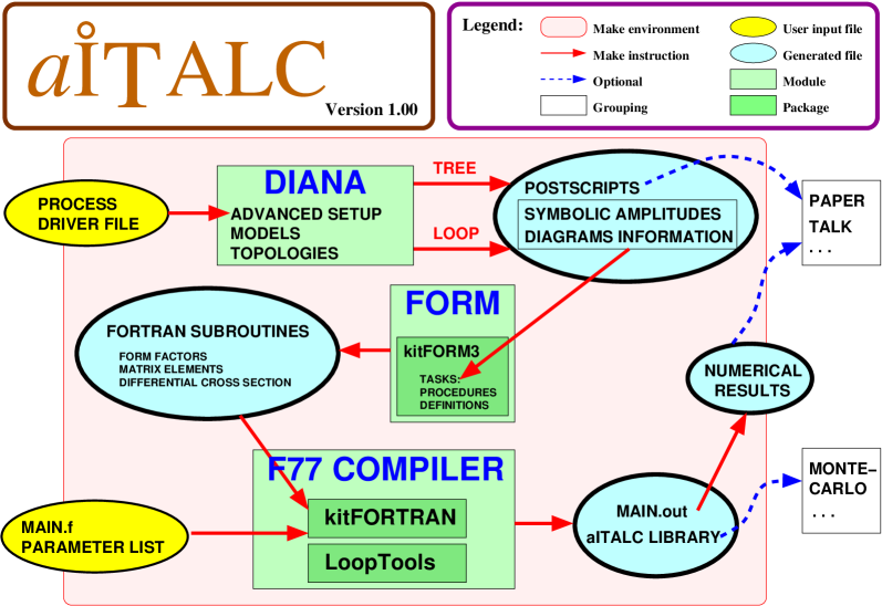
Figure 1: Flow chart of the ai̊Talc package.

The package ai̊Talc for the automatic calculation of a variety of two fermion production processes may be obtained from [6] where also its installation will be described. The logical structure of the package is shown in Figure 1. It consists of three modules: Diana, kitForm3 and kitFortran. In order to run and/or modify one of the samples in the example directory, the user has to choose the process in terms of incoming and outgoing fermions and the model lagrangian; we support two models: QED.model and EWSM.model, both with counterterms. This is done by modifying the driver file process.ini in the sample directory tree. Sample processes are: Bhabha scattering (eeee), $\mu$ pairs (muon_production), $b$ pairs (eebb), $b\bar{s}$ (leLe-bS), $t\bar{c}$ (leLe-tC), etc. Selected cases will also be part of the public distribution.

The electroweak corrections are organized following [7, 8], and we keep all the fermion masses, including $m_{e}$, by default.

The user runs the package by Make in e.g. eebb_user and produces (among others) the subdirectories tree, loop and fortran. The Diana module uses Qgraf v.2.0 [9] and Diana v.2.35 [10] and creates symbolic Form-readable output for each of the Feynman diagrams in eebb.in. Moreover, graphical representations are produced, both stored as encapsulated postscript figures in EPS (single Feynman diagrams) and as postscripts in eebbInfo.ps (with detailed informations for each single diagram) and in eebb.ps (an overview of all contributions).

Then module kitForm3 performs some algebraic simplifications and determines the matrix elements and form factors. This operation takes place separately for the tree and loop levels. The module kitFortran returns the Fortran executable file main.out and the library libaitalc_v1.a. Two Fortran files, parameterlist.hf and main.f, provide the user access to the input parameters in the model and to the design of numerical output of the code (i.e. number of data points in the angular distribution, integrated cross section, running flags, etc.). By executing main.out, the user produces a sample output main.log with differential and integrated cross sections, as well as forward-backward asymmetries. For Bhabha scattering at $\sqrt{s}=500$ GeV, a shortened sample is reproduced in Table 1.

Advanced features are not extremely user friendly, but are still under development. Soft photonic corrections may be included (or not), and with lidentCKM=.true. quark flavour mixing is discarded with a diagonal CKM matrix. One may also perform a full one-loop tensor integral reduction to the master integrals $A_{0}$, $B_{0}$, $C_{0}$ and $D_{0}$ in the Passarino-Veltman scheme [11]. All these possibilities will be described in more detail in a tutorial to be published soon; see also [12].

3 SELECTED APPLICATIONS

3.1 Bhabha scattering

Bhabha scattering,

$$e^{+}e^{-}\rightarrow e^{+}e^{-},$$ (2)

was one of the first processes to be calculated in QED [13], and the one-loop corrections in the SM were treated in [14, 15, 16, 17, 18, 19, 20].

We are calculating the virtual corrections to massive, low angle Bhabha scattering at a Linear Collider [1]. In order to guarantee a precision of $10^{-4}$ of the differential cross section we need the one-loop corrections in the SM, and the two-loop corrections in pure, massive QED [21]; the latter comprise also the squared one-loop corrections [22].

The one-loop SM corrections are determined with ai̊Talc. A shortened example of the ai̊Talc output is given in Table 1. A comparison of our calculation with another one based on FormCalc [23] is reproduced in [12], where an agreement is obtained of more than 12 significant digits.

Table 1: Sample output of ai̊Talc for Bhabha scattering at $\sqrt{s}=500$ GeV: Born and 1-loop corrected differential cross sections; input data as in [3, 12]

# ==================================================================
# aITALC: Version 0.7 by A.Lorca -- T.Riemann
# ==================================================================
#cos(theta) dcs(BORN)               ...  dcs(BORN+Q+W+soft)      ...
-.90000     0.2169988288109205E+00  ...  0.1934450785268578E+00  ...
-.50000     0.2613604305853236E+00  ...  0.2387066977233451E+00  ...
0.00000     0.5981423072503301E+00  ...  0.5466771794694227E+00  ...
0.50000     0.4212729493916255E+01  ...  0.3813007881789546E+01  ...
0.90000     0.1891603223322704E+03  ...  0.1729283490665079E+03  ...
# ------------------------------------------------------------------

3.2 At the $Z$-peak

For the numerical evaluation of the one-loop functions we use LoopTools v.2.0 and follow the conventions given in the manual [24, 25, 26]. LoopTools relies on the package FF [25]. In contrast to FF, it does not support the case of complex masses. Near the $Z$-peak, the Breit-Wigner $Z$ propagator has to be used,

$$\frac{1}{s-m_{Z}^{2}+i\varepsilon}\rightarrow\frac{1}{s-m_{Z}^{2}+i\Gamma_{Z}m_{Z}},$$ (3)

with a width parameter $\Gamma_{Z}$. Flag lwidth activates the following changes in ai̊Talc:

• Apply substitution (3) in Feynman rules;

• Avoid double counting by discarding the $Z$ self-energy diagrams resummed in $\Gamma_{Z}$;

• Use loop integrals with complex $Z$ mass.

In general we use for the numerics Passarino-Veltman functions of scalar, vector, and tensor type. In the neighbourhood of the $Z$ resonance, though, we perform the tensor reduction for the $\gamma-Z$ dependent functions $D_{ij}(...)$, and have to calculate the following functions with complex $Z$ mass: $B_{0}$, $C_{0}$ and $D_{0}$. The $A_{0}$ and $B_{0}$ are trivial, and the infrared divergent $D_{0}$ was calculated in [27]. The tensor reduction of the tensor integrals related to the $\gamma-Z$ box diagrams leads, by shrinking of internal lines, to infrared safe two- and three-point functions with complex $Z$ mass. They are generally treated in [28] and available in the FF package [25]. We performed an independent calculation of the only nontrivial one, $C_{0}(\ldots;m_{Z}^{2}-i\Gamma_{Z}m_{Z},0,m_{f}^{2})$, and got perfect agreement with FF. For an implementation and comparison between the non-width and width cases see Figure 2.

As an example, the differential cross section for $e^{+}e^{-}\to\mu^{+}\mu^{-}$ around the $Z$-peak is presented in Figure 3.

3.3 Flavour number violation

Topics of particular interest are flavour changing neutral current processes at $e^{+}e^{-}$ colliders since they are forbidden in the Born approximation of the Standard Model and might indicate New Physics. At one-loop order, they may occur in the SM if the fermions of different flavour have different masses and are mixing. Usually one calculates simply the flavour changing $Z$ decay rate because the chances to observe an effect are largest at the $Z$-peak. The predictions in the minimally extended Standard Model are tiny (see e.g. [29, 30, 31]), but may be much larger with supersymmetry (see e.g. [32]). Recently, there were also studies of the complete scattering processes [33, 34]:

$$e^{+}e^{-}\to t\bar{c},\quad b\bar{s}.$$ (4)

The mass effects, but also both $Z$ and $\gamma$ exchange, and the $WW$ box are taken into account. We recalculated the corresponding rates with ai̊Talc. Figure 4 shows our differential cross sections for (4). By inspection of the corresponding plot in [34], one realizes a normalization difference of about $3/2$ or $\pi/2$ by which our cross section is larger. Using the input data of [34], we get:

$$\sigma_{b{\bar{s}}}(\sqrt{s}=m_{Z}) = (1.136\pm 0.001)\;\mathrm{f{}b},$$

$$\sigma_{b{\bar{s}}}(\sqrt{s}=200\mathrm{GeV}) = (2.033\pm 0.002)\;\mathrm{f{}b}.$$

For the other channel, we agree within the accuracy of the figures. Figure 5 shows also the total cross section for $b\bar{s}$.

Figure 2: The infrared finite function $C_{0}(s,m_{\mu}^{2},m_{\mu}^{2};m_{Z}^{2},0,m_{\mu}^{2})$ as a function of $\sqrt{s}$.

Figure 3: Muon production at the $Z$-peak.

Figure 4: Differential cross sections for $e^{+}e^{-}\rightarrow b\bar{s}$ and $e^{+}e^{-}\rightarrow t\bar{c}$ at $\sqrt{s}=200$ GeV; input data as in [34].

Figure 5: Integrated cross section for $e^{+}e^{-}\rightarrow b\bar{s}$ as a function of $\sqrt{s}$; input data as in [33].

4 CONCLUDING REMARKS

We plan to include into ai̊Talc also processes which have contributions from Feynman diagrams with five-point functions. This would allow us to calculate the one-loop corrections to the radiative Bhabha process, $e^{+}e^{-}\to e^{+}e^{-}\gamma$.

Further, it would be very important to have a proper treatment of Majorana particles with Qgraf and Diana, thus allowing also the treatment of supersymmetric model files.

References

- [1] ECFA/DESY LC Physics Working Group, J. Aguilar-Saavedra et al., hep-ph/0106315.
- [2] J. Fleischer et al., Eur. Phys. J. C31 (2003) 37, hep-ph/0302259.
- [3] T. Hahn et al., hep-ph/0307132.
- [4] J. Gluza, A. Lorca and T. Riemann, Contribution to ACAT03, to appear in Nucl. Instrum. Meth.; see [35].
- [5] A. Biernacik et al., Acta Phys. Polon. B34 (2003) 5487, hep-ph/0311097.
- [6] A. Lorca and T. Riemann, http://www-zeuthen.desy.de/theory/research/aitalc.
- [7] A. Denner, Fortschr. Phys. 41 (1993) 307.
- [8] M. Böhm et al., Fortsch. Phys. 34 (1986) 687.
- [9] P. Nogueira, J. Comput. Phys. 105 (1993) 279.
- [10] M. Tentyukov and J. Fleischer, Nucl. Instrum. Meth. A502 (2003) 570.
- [11] G. Passarino and M. Veltman, Nucl. Phys. B160 (1979) 151.
- [12] A. Lorca, http://www-zeuthen.desy.de /~alorca/downloads/montpellier-11-03.pdf.
- [13] H. Bhabha, Proc. Roy. Soc. A154 (1936) 195.
- [14] M. Consoli, Nucl. Phys. B160 (1979) 208.
- [15] M. Böhm et al., Phys. Lett. B144 (1984) 414.
- [16] K. Tobimatsu and Y. Shimizu, Prog. Theor. Phys. 75 (1986) 905.
- [17] D. Bardin, W. Hollik and T. Riemann, Z. Phys. C49 (1991) 485.
- [18] W. Beenakker, F. Berends and S. van der Marck, Nucl. Phys. B349 (1991) 323.
- [19] G. Montagna et al., Nucl. Phys. B401 (1993) 3.
- [20] W. Beenakker and G. Passarino, Phys. Lett. B425 (1998) 199, hep-ph/9710376.
- [21] M. Czakon, J. Gluza and T. Riemann, hep-ph/0406203, to appear in Proc. of DESY Workshop “Loops and Legs in Quantum Field Theory”, April 25-30, 2004, Zinnowitz, Germany, Nucl. Phys. B (Proc. Suppl.).
- [22] J. Fleischer et al., Nucl. Instrum. Meth. A502 (2003) 567, hep-ph/0210180.
- [23] T. Hahn, The FormCalc Homepage, http://www.feynarts.de/formcalc .
- [24] T. Hahn et al., Comput. Phys. Commun. 118 (1999) 153, hep-ph/9807565.
- [25] G.J. van Oldenborgh, Comput. Phys. Commun. 66 (1991) 1.
- [26] T. Hahn, “LoopTools User’s Guide”, http://www.feynarts.de/looptools .
- [27] W. Beenakker and A. Denner, Nucl. Phys. B338 (1990) 349.
- [28] G. ’t Hooft and M. Veltman, Nucl. Phys. B153 (1979) 365.
- [29] G. Mann and T. Riemann, Annalen Phys. 40 (1984) 334.
- [30] V. Ganapathi et al., Phys. Rev. D27 (1983) 579.
- [31] J.I. Illana and T. Riemann, Phys. Rev. D63 (2001) 053004, hep-ph/0010193.
- [32] J.I. Illana and M. Masip, Phys. Rev. D67 (2003) 035004, hep-ph/0207328.
- [33] C. Huang, X. Wu and S. Zhu, Phys. Lett. B452 (1999) 143, hep-ph/9901369.
- [34] C. Huang, X. Wu and S. Zhu, J. Phys. G25 (1999) 2215, hep-ph/9902474.
- [35] M. Czakon et al., http://www-zeuthen.desy.de/theory/research/bhabha.