A probability measure in the space of spectral functions and structure functions

Abstract

We present a novel technique to parametrize experimental data, based on the construction of a probability measure in the space of functions, which retains the full experimental information on errors and correlations. This measure is constructed in a two step process: first, a Monte Carlo sample of replicas of the experimental data is generated, and then an ensemble of neural network is trained over them. This parametrization does not introduce any bias due to the choice of a fixed functional form. Two applications of this technique are presented. First a probability measure in the space of the spectral function $\rho_{V-A}(s)$ is generated, which incorporates theoretical constraints as chiral sum rules, and is used to evaluate the vacuum condensates. Then we construct a probability measure in the space of the proton structure function $F_{2}^{p}(x,Q^{2})$, which updates previous work, incorporating HERA data.

1 Introduction and motivation

The general problem we are considering here is that of the parametrization of experimental data. This is an ill-posed problem, since it consists on obtaining continuous functions from a finite set of measurements. Standard parameterizations, which consist on choosing a functional form and fitting its parameters to the data, have a series of shortcomings: first, the choice of a functional form introduces an a priori bias, which implies a theoretical uncertainty whose size is very difficult to asses. Another important problem is how errors and correlations are represented within this parametrization, and how uncertainties are propagated to other observables, since linear error propagation is not trustable in general.

The motivation for this problem is the issue of Parton Distributions Functions (PDFs) for the LHC [1]. Recently, a considerable amount of theoretical and experimental effort has been invested in their accurate determination, and in particular their associate errors, in view of the accurate computation of collider processes and determination of QCD parameters. On the theory side, the PDFs should be unbiased with respect to the choice of functional form, and moreover the full experimental information should be incorporated into the PDFs parametrization, including systematic errors and correlations in a way that allows it to propagate to observables (like cross sections) without introducing an additional bias, linear approximations for instance. The technique that we present here is specially devised to fulfill all these requirements.

2 General strategy

In this section we review the approach we take to this problem [2]. The basic idea is to construct a probability measure in the space of functions, ${\mathcal{P}}\left[f\right]$, from experimental information for $f$. From this probability measure one can compute any observable and the associated uncertainty and correlation, using weighted averages

$$\left\langle{\mathcal{F}}\left[f(\vec{x})\right]\right\rangle=\int{\mathcal{D}}f{\mathcal{F}}\left[f(\vec{x})\right]{\mathcal{P}}\left[f\right]\ .$$ (1)

The way this idea is implemented in our formalism is using neural networks as universal unbiased interpolants, in a two step process. The first step is the Monte Carlo sampling, where we generate a number of replicas of the artificial. Then we train an ensemble of neural networks over these generated replicas. The whole procedure is then validated through suitable statistical estimators.

The first step is the Monte Carlo sampling of experimental data, which consists on the generation of $N_{rep}$ Monte Carlo sets of ’pseudo-data’, replicas of the original $N_{dat}$ data points, $f_{i}^{(art)(k)}$, $i=1,\ldots,N_{dat}$,$k=1,\ldots,N_{rep}$ using equations of the form

$$f_{i}^{(art)(k)}=\Delta_{N}\Big{[}f_{i}^{(exp)}+r_{i}^{s}\sigma^{stat}_{i}+\sum_{l=1}^{N_{sys}}r^{l,(k)}\sigma_{i}^{sys,l}\Big{]}\ ,$$ (2)

where $\sigma_{i}^{stat}$ and $\sigma_{i}^{sys,l}$ are the statistical and the different systematic errors of the point $i$ and $\Delta_{N}\equiv\left(1+r_{N}^{(k)}\sigma_{N}\right)$ is the contribution from the normalization error. The $r_{i}$ are univariate gaussian random numbers. Correlated systematics share the same random numbers, and this takes into account the correlations in the generation of the replicas.

The second part of our technique consists on training one neural network [3] on each Monte Carlo replica of the experimental data. Neural networks are useful for our purposes since they are the most unbiased prior, and they are robust, unbiased universal approximants, so using them eliminates the need of introducing a bias by choosing a functional form for our parametrization. We use a combination of two different techniques for training the networks: Backpropagation (BP) learning and Genetic Algorithms (GA) learning. The second technique, inspired in evolutionary models in in biology, has been widely used in other branches of science. In this context training means the minimization of an error function evaluated with the covariance matrix for each replica

$$E^{(k)}=\sum_{i,j=1}^{N_{dat}}\Delta f_{i}^{(k)}{\mathrm{c}ov}^{-1}_{ij}\Delta f_{j}^{(k)}\ ,$$ (3)

where $\Delta f_{i}^{(k)}\equiv f_{i}^{(art)(k)}-f_{i}^{(net)(k)}$, so that this error function measures the goodness of the fit. The set of trained nets is the sought-for probability measure in the space of functions $f$, and defines a parametrization of the experimental information for $f$. Averages over this probability measure are performed using

$$\left\langle{\mathcal{F}}\left[f_{i}\right]\right\rangle=\frac{1}{N_{rep}}\sum_{k=1}^{N_{rep}}{\mathcal{F}}\left[f^{(net)(k)}_{i}\right]\ .$$ (4)

The final step consists on the validation of the fitting process using statistical estimators.

3 Spectral functions

Now we turn to consider the first of the two applications [4] of this technique. The vector and axial-vector spectral functions $v_{1}(a),a_{1}(s)$ have been measured in hadronic tau decays at LEP (ALEPH [5] and OPAL) up to $s=M_{\tau}^{2}$ with large precision except near threshold. In particular we are interested in parameterizing the vector-axial vector spectral function $~{}\rho_{V-A}(s)\equiv v_{1}(s)-a_{1}(s)$. This spectral function is interesting since it vanishes to all orders in perturbation theory, and thus is specially suited to study nonperturbative aspects of QCD. In particular this spectral function is an order parameter of spontaneous chiral symmetry breaking.

The combined use of the operator product expansion and dispersion relations [6] allows an extraction of the QCD vacuum condensates in terms of convolutions of this spectral function,

$$~{}\left\langle{\mathcal{O}}_{2n+2}\right\rangle=(-1)^{n}\int_{0}^{\infty}dss^{n}\frac{1}{2\pi^{2}}\rho_{V-A}(s)\ .$$ (5)

However, there are problems with experimental data to obtain a clean extraction. First of all, we have information only up to the tau mass kinematic threshold $s=M_{\tau}^{2}$, and second, there are large errors and correlations near this threshold due to phase space suppression factors. One possible solution consists on constructing a probability measure in the space of spectral functions $\rho_{V-A}(s)$ using the general technique introduced above and then use the  chiral sum rules to constrain the large $s$ behavior within this probability measure.

Now we proceed as explained in Section 2. The only difference in the GA training epoch consists on the minimization for each replica of a modified error function,

$$E^{(k)}+\sum_{l=1}^{4}g_{l}\left(\int_{0}^{\infty}dsf_{l}(\rho_{V-A}^{(k)})-A_{l}\right)^{2}+E^{(k)}[s_{0}]$$ (6)

which takes into account both the theoretical constraints from the chiral sum rules (second term) and the asymptotic constraint $\rho_{V-A}(s\to\infty)=0$ (third term). The chiral sum rules [7] that are incorporated into the probability measure are the Das-Mathur-Okubo sum rule, the first and the second Weinberg sum rules (WSR), and the electromagnetic mass splitting of the pion sum rule. The use of GA is crucial here since allows the learning of non-local error functions like Eq. 6.

So using this technique the probability measure for $\rho_{V-A}(s)$ is constructed, and from this measure we can evaluate any observable with the corresponding uncertainty. The results for the lower dimensional condensates are $\left\langle{\mathcal{O}}_{6}\right\rangle=\left(-4.0~{}\pm 2.0\right)~{}10^{-3}~{}\mathrm{GeV}^{6}$ and $\left\langle{\mathcal{O}}_{8}\right\rangle=\left(-12~{}\hbox{${\lower 1.0pt\hbox{$\scriptstyle+~{}7$}}\atop{\raise 1.0pt\hbox{$\scriptstyle-~{}11$}}$}\right)10^{-3}~{}\mathrm{GeV}^{8}$ (see Fig. 1). While the result of $\left\langle{\mathcal{O}}_{6}\right\rangle$ is standard, the sign of $\left\langle{\mathcal{O}}_{8}\right\rangle$ oscillates in the literature [8]. We find that the uncertainties in the determination of the condensates are often underestimated and dominated by theoretical (model-dependent) uncertainties.

Figure 1: The $\left\langle{\mathcal{O}}_{6}\right\rangle$ condensate as a function of $s_{0}$. Error bands show propagation of experimental uncertainties.

4 Structure functions

Now we present the second application [9], a parametrization of the proton structure function $F_{2}^{p}(x,Q^{2})$, which is an update of Ref. [2], with the following novel features: incorporation of 11 more experiments (E665, H1 and ZEUS, in addition to NMC and BCDMS), direct minimization of covariance matrix error function and an improved analysis of experimental uncertainties (like a dedicated treatment of asymmetric errors and uncorrelated systematics). Note that a single fit covers the whole kinematical range, $6~{}10^{-7}\leq x\leq 0.8$, $4.5~{}10^{-2}\leq Q^{2}\leq 3~{}10^{4}~{}\mathrm{GeV}^{2}$, which consists on regions with very different behaviour, since we do not need to supply any functional form.

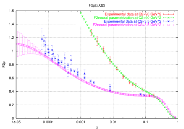
Figure 2: Comparison of the F2neural fit with experimental data. Only diagonal errors are shown, point-to-point correlations might be large.

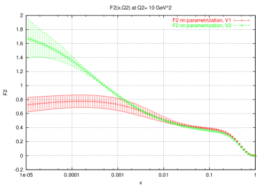
Figure 3: Comparison of old and new versions of the F2neural fit. Note the characteristic increase of uncertainty in regions without experimental data

Following the steps of Section 2, we obtain a parametrization for $F_{2}^{p}(x,Q^{2})$. In Fig. 2 one can observe our parametrization compared with experimental data. Note that the uncertainties in $F_{2}^{p}(x,Q^{2})$ are automatically incorporated in the parametrization. Note also a relevant feature: in regions without experimental data, the uncertainties increases in a very characteristic way, so the region where the parametrization ceases to be trustable is under control.

It is interesting to study the effect of the incorporation of new experiments by comparing our parametrization with the old version of F2neural [2], where the only experimental data was from the NMC and BCDMS experiments (see Fig. 3). Note that the two fits are consistent in the region with same experimental data (high $x$ region) but differ at low $x$ where the new fit is better, as was expected since incorporates the HERA data.

5 Conclusions and future work

We have presented a general technique to parametrize experimental data, applying it to two different problems. We have constructed a probability measure in the space of spectral functions and structure functions showing that additional theoretical constraints (sum rules, kinematical constraints) can be incorporated in the probability measure. These two applications increase the confidence on the validity of our approach. The next step is to construct a probability measure in the space of PDFs, with full control over experimental uncertainties, accurate error propagation and no bias due to the choice of fixed functional forms.

Acknowledgements

We would like to thank the QCD04 Conference organizers. This work has been supported by the projects MCYT FPA2001-3598, GC2001SGR-00065 and by the Spanish grant AP2002-2415.

References

- [1] See S. Forte, Nucl. Phys. A 666 (2000) 113; S. Catani et al., [arXiv:hep-ph/0005025]; R. D. Ball and J. Huston, in S. Catani et al., [arXiv:hep-ph/0005114] and ref. therein.
- [2] S. Forte, L. Garrido, J. I. Latorre and A. Piccione, JHEP 0205, 062 (2002) [arXiv:hep-ph/0204232].
- [3] B. Müller, J. Reinhardt and M. T. Strickland, ”Neural Networks: an introduction”.
- [4] J. Rojo and J. I. Latorre, JHEP 0401, 055 (2004) [arXiv:hep-ph/0401047].
- [5] R. Barate et al. [ALEPH Collaboration], Eur. Phys. J. C 4, 409 (1998).
- [6] M. A. Shifman, A. I. Vainshtein and V. I. Zakharov, Nucl. Phys. B 147, 385 (1979), E. Braaten, S. Narison and A. Pich, Nucl. Phys. B 373, 581 (1992).
- [7] T. Das, V.S. Mathur and S. Okubo, Phys. Rev. Lett. 19 (1967) 895; S. Weinberg, Phys. Rev. Lett. 18 (1967) 507; T. Das, G.S. Guralnik, V.S. Mathur, F.E. Low and J.E. Young, Phys. Rev. Lett. 18 (1967) 759.
- [8] J. Bijnens, E. Gamiz and J. Prades, JHEP 0110 009 (2001); M. Knecht, S. Peris and E. de Rafael, Phys. Lett. B508 (2001) 117; V. Cirigliano, E Golowich and K Maltman, Phys.Rev. D68 (2003) 054013.
- [9] A. Piccione, J. Rojo, L. Del Debbio, S. Forte, L. Garrido, J. I Latorre, work in preparation.