Weak Corrections to Hadronic Observables

Abstract

We illustrate one-loop weak corrections to three-jet production in $e^{+}e^{-}$ at $\sqrt{s}=M_{Z}$, to the production of a $Z$ or $\gamma$ in association with a hard jet at hadron colliders and to the production cross section of two $b$-jets at Tevatron and Large Hadron Collider (LHC).

E. Mainato, S. Morettisouthampton, M.R. Noltensouthampton, D.A. Rosssouthampton.

toUniversità di Torino and INFN, Torino, Italy southamptonUniversity of Southampton, Southampton, UK

1 Introduction

One-loop EW corrections, as compared to the QCD ones, have a relatively large impact. This can be understood (see Refs. [1]–[2] and references therein for reviews) in terms of the so-called Sudakov (leading) logarithms of the form $\alpha_{\mathrm{W}}\log^{2}(\sqrt{\hat{s}}/M_{W}^{2})$, which appear in the presence of higher order weak corrections (hereafter, $\alpha_{\rm{W}}\equiv\alpha_{\rm{\small EM}}/\sin^{2}\theta_{\rm W}$, with $\alpha_{\rm{\small EM}}$ the Electro-Magnetic (EM) coupling constant and $\theta_{\rm W}$ the weak mixing angle). These ‘double logs’ are due to a lack of cancellation of infrared (both soft and collinear) virtual and real emission in higher order contributions due to $W$-exchange in spontaneously broken non-Abelian theories.

The problem is, in principle, present also in QCD. In practice, however, it has no observable consequences, because of the averaging on the colour degrees of freedom of partons, forced by their confinement into colourless hadrons. This does not occur in the EW case, where, e.g., the initial state can have a non-Abelian charge, dictated by the given collider beam configuration. Modulo the effects of the Parton Distribution Functions (PDFs), which spoil the subtle cancellations among subprocesses with opposite non-Abelian charge, for example, this argument holds for an initial quark doublet in proton-(anti)proton scatterings. These logarithmic corrections (unless the EW process is mass-suppressed) are universal (i.e., process independent) and are finite (unlike in QCD), as the masses of the EW gauge bosons provide a physical cut-off for $W$-boson emission. Hence, for typical experimental resolutions, softly and collinearly emitted weak bosons need not be included in the production cross-section and one can restrict oneself to the calculation of weak effects originating from virtual corrections. In fact, one should recall that real weak bosons are unstable and decay into high transverse momentum leptons and/or jets, which are normally captured by the detectors. In the definition of an exclusive cross section then, one tends to remove events with such additional particles. Under such circumstances, the (virtual) exchange of $Z$-bosons also generates similar logarithmic corrections, $\alpha_{\mathrm{W}}\log^{2}(\sqrt{\hat{s}}/M_{Z}^{2})$. Besides, the genuinely weak contributions can be isolated in a gauge-invariant manner from purely EM effects, at least in some simpler cases – which do include the processes discussed hereafter – and the latter may or may not be included in the calculation, depending on the observable being studied.

A further aspect that should be recalled is that weak corrections naturally introduce parity-violating effects in observables, detectable through asymmetries in the cross-section, which are often regarded as an indication of physics beyond the Standard Model (SM) [3, 4, 5]. These effects are further enhanced if polarisation of the incoming beams is exploited, such as at RHIC-Spin [6, 7] or a future Linear Collider(LC). Comparison of theoretical predictions involving parity-violation with experimental data is thus used as another powerful tool for confirming or disproving the existence of some beyond the SM scenarios, such as those involving right-handed weak currents [8], contact interactions [9] and/or new massive gauge bosons [10, 11].

In view of all this, it becomes of crucial importance to assess the quantitative relevance of weak corrections.

Figure 1: Self-energy insertion graphs. The shaded blob on the incoming wavy line represents all the contributions to the gauge boson self-energy and is dependent on the Higgs mass (hereafter, we will use $M_{H}=115$ GeV for the latter). In this and all subsequent figures the graphs in which the exchanged gauge boson is a $W$-boson is accompanied by corresponding graphs in which the $W$-boson is replaced by its corresponding Goldstone boson. Since the Yukawa couplings are proportional to the fermion masses, such graphs are only significant in the case of $b$-quark jets. There is a similar set of diagrams in which the direction of the fermion line is reversed.

2 Calculation

Since we are considering weak corrections that can be identified via their induced parity-violating effects and since we wish to apply our results to the case of polarised electron and/or positron beams, it is convenient to work in terms of helicity matrix elements (MEs). Thus, we define the helicity amplitudes ${\cal A}^{(G)}_{\lambda_{1},\lambda_{2},\sigma}$ for the process

$$V(q_{1})+q(p_{1})\rightarrow g(q_{2})+q(p_{2}),$$ (1)

the scattering of a gauge boson of type $G$ (hereafter, a possibly virtual photon $\gamma^{*}$ or a $Z$-boson) of helicity $\lambda_{1}$ and a quark with helicity $\sigma$ into a gluon with helicity $\lambda_{2}$ and a massless quark with the same helicity $\sigma$.. The EW boson can have a longitudinal polarisation component, so that the helicity $\lambda_{1}$ can take three values, $\pm 1,\,0$, for both the $\gamma^{*}$ and $Z$ gauge vectors, whereas $\lambda_{2}$ and $\sigma$ can only be equal to $\pm 1$.

The general form of these amplitudes may be written as

$${\cal A}^{(G)}_{\lambda_{1},\lambda_{2},\sigma}\ =\ \bar{u}(p_{2})\Gamma\frac{\left(1+\sigma\gamma^{5}\right)}{2}u(p_{1})$$ (2)

where $p_{1}$ and $p_{2}$ are the momenta of the incoming and outgoing quark respectively and $\Gamma$ stands for a sum of strings of Dirac $\gamma-$matrices with coefficients, which, beyond tree level, involve integrals over loop momenta. Since the helicity $\sigma$ of the fermions is conserved the strings must contain an odd number of $\gamma-$matrices. Repeated use of the Chisholm identity means that $\Gamma$ can always be expressed in the form

$$\Gamma\ =\ C_{1}\,\gamma\cdot p_{1}\ +\ C_{2}\,\gamma\cdot p_{2}\ +\ C_{3}\,\gamma\cdot q_{2}\ +\ C_{4}\,\sqrt{Q^{2}}\,\gamma\cdot n,$$ (3)

where $q_{2}$ is the momentum of the outgoing gluon, $Q^{2}=q_{1}^{2}$ is the square momentum of the gauge boson, and $n$ is a unit vector normal to the quark and gluon momenta, more precisely:

$$n_{\mu}=\frac{1}{\sqrt{2~{}p_{1}\cdot p_{2}~{}p_{1}\cdot q_{2}~{}p_{2}\cdot q_{2}}}\varepsilon_{\mu\nu\rho\sigma}p_{1}^{\nu}p_{2}^{\rho}q_{2}^{\sigma}.$$ (4)

The coefficient functions $C_{i}$ depend on the helicities $\lambda_{1},\ \lambda_{2},\ \sigma$ as well all independent kinematical invariants and on all the couplings and masses of particles that enter into the relevant perturbative contribution to the amplitude.

For massless fermions the MEs of the first two terms of eq. (3) vanish, and we are left with

$$\ {\cal A}^{(G)}_{\lambda_{1},\lambda_{2},\sigma}=C_{3}\,\bar{u}(p_{2})\gamma\cdot q_{2}\frac{\left(1+\sigma\gamma^{5}\right)}{2}v(p_{1})\,+\,C_{4}\sqrt{Q^{2}}\,\bar{u}(p_{2})\gamma\cdot n\frac{\left(1+\sigma\gamma^{5}\right)}{2}v(p_{1}),$$

The relevant coefficient functions $C_{3}$ and $C_{4}$ are scalar quantities and can be projected on a graph-by-graph basis using the projections

$$C_{3}\ =\ {\rm Tr}\left(\Gamma\gamma\cdot v\frac{\left(1+\sigma\gamma^{5}\right)}{2}\right)$$ (5)

where $v$ is the vector

$$v^{\mu}\ =\ =\frac{1}{-u}p_{1}^{\mu}\,+\,\frac{1}{s}p_{2}^{\mu}-\frac{-t}{-u\,s}q_{2}^{\mu}$$ (6)

with $s=(p_{1}+q_{1})^{2},\quad t=(p_{2}-p_{1})^{2},\quad u=(q_{2}-p_{1})^{2}$ and

$$C_{4}\ =\ -\frac{1}{2\sqrt{Q^{2}}}{\rm Tr}\left(\Gamma\gamma\cdot n\frac{\left(1+\sigma\gamma^{5}\right)}{2}\right).$$ (7)

The basic matrix elements read

$$\bar{u}(p_{2},\sigma)(\gamma\cdot q_{2})u(p_{1},\sigma)\ =\ \sqrt{-u\,s}\quad\quad\bar{u}(p_{2},\sigma)(\gamma\cdot n)u(p_{1},\sigma)\ =\ -i\,\sigma\,\sqrt{-t\,s}$$ (8)

Figure 2: Vertex correction graphs. Again, same considerations as in the previous figure apply for the case of Goldstone bosons and there is a similar set of graphs in which the direction of the fermion line is reversed

Figure 3: Box graphs. Again, same considerations as in the previous two figures apply for the case of Goldstone bosons. Here, the first graph is accompanied by a similar graph with the direction of the fermion line reversed whereas for the second graph this reversal does not lead to a distinct Feynman diagram.

At one-loop level such helicity amplitudes acquire higher order corrections from the self-energy insertions on the fermions and gauge bosons shown in Fig. 1, from the vertex corrections shown in Fig. 2 and from the box diagrams shown in Fig. 3. As we have neglected here the masses of the external quarks, such higher order corrections depend on the ratio $Q^{2}/M_{{W}}^{2}$, where $Q^{2}$ is the square momentum of the gauge boson, as well as the EM coupling constant $\alpha_{\rm EM}$ and the weak mixing angle $s_{W}\equiv\sin\theta_{W}$ (with $\alpha_{\rm EW}=\alpha_{\rm EM}/s_{W}^{2}$). Furthermore, in the case where the external fermions are $b$-quarks, the loops involving the exchange of a $W$-boson lead to effects of virtual $t$-quarks, so that the corrections also depend on the ratio $m_{t}^{2}/M_{{W}}^{2}$. (It is only in this case that the graphs involving the exchange of the Goldstone bosons associated with the $W$-boson graphs are relevant.)

The self-energy and vertex correction graphs contain ultraviolet divergences. These have been subtracted using the ‘modified’ Minimal Subtraction ($\overline{\mathrm{MS}}$) scheme at the scale $\mu=M_{Z}$. Thus the couplings are taken to be those relevant for such a subtraction: e.g., the EM coupling, $\alpha_{\mathrm{EM}}$, has been taken to be $1/128$ at the above subtraction point. Two exceptions to this renormalisation scheme have been the following:

1. the self-energy insertions on external fermion lines, which have been subtracted on mass-shell, so that the external fermion fields create or destroy particle states with the correct normalisation;

2. the mass renormalization of the $Z$-boson propagator, which has also been carried out on mass-shell, so that the $Z$ mass does indeed refer to the physical pole-mass.

All these graphs are infrared and collinear convergent so that they may be expressed in terms of Passarino-Veltman [12] functions which are then evaluated numerically. The expressions for each of these diagrams have been calculated using FORM [13] and checked by an independent program based on FeynCalc [14]. For the numerical evaluation of the scalar integrals we have relied on FF [15]. A further check on our results has been carried out by setting the polarisation vector of the photon proportional to its momentum and verifying that in that case the sum of all one-loop diagrams vanishes, as required by gauge invariance.

3 Results

3.1 Factorisable Corrections to Three-Jet Production in Electron-Positron Annihilations[16]

Figure 4: The $A(y)$, $-A_{\mathrm{W}}$ and $B(y)$ coefficient functions of eqs. (11)–(12) for the Geneva and Jade jet clustering algorithms, at $\sqrt{s}=M_{Z}$. (Notice that the $\sim A_{\mathrm{W}}$ term has been plotted with opposite sign for better presentation.)

Here we report on the computation of one-loop weak effects entering three-jet production in electron-positron annihilation

$$e^{+}e^{-}\to\gamma^{*},Z\to\bar{q}qg\quad{\mathrm{(all~{}flavours)}},$$ (9)

when no assumption is made on the flavour content of the final state, so that a summation will be performed over $q=d,u,c,s,b$-quarks, and also

$$e^{+}e^{-}\to\gamma^{*},Z\to\bar{b}bg,$$ (10)

limited to the case of bottom quarks only in the final state. We restrict our attention to $\sqrt{s}=M_{Z}$ , when the higher order effects arise only from initial or final state interactions. These represent the so-called ‘factorisable’ corrections, i.e., those involving loops not connecting the initial leptons to the final quarks, which are the dominant ones at $\sqrt{s}=M_{Z}$ (where the width of the $Z$ resonance provides a natural cut-off for off-shellness effects). The remainder, ‘non-factorisable’ corrections, while being negligible at $\sqrt{s}=M_{Z}$, are expected to play a quantitatively relevant role as $\sqrt{s}$ grows larger. As a whole, one-loop weak effects will become comparable to QCD ones at future LCs running at TeV energy scales. In contrast, at the $Z$ mass peak, where no logarithmic enhancement occurs, one-loop weak effects are expected to appear at the percent level, hence being of limited relevance at LEP1 and SLC, where the final error on $\alpha_{\mathrm{S}}$ is of the same order or larger [20], but of crucial importance at a GigaZ stage of a future LC, where the relative accuracy of $\alpha_{\mathrm{S}}$ measurements is expected to be at the $0.1\%$ level or smaller [21].

Figure 5: The total cross section for process (10) at LO and NLO-W for the Cambridge, Durham, Geneva and Jade jet clustering algorithms, at $\sqrt{s}=M_{Z}$. (Notice that the NLO-W results have been plotted with opposite sign for better presentation.)

For the choice $\mu=\sqrt{s}$ of the renormalisation scale, one can conveniently write the three-jet fraction in the following form:

$$R_{3}(y)=\left(\frac{\alpha_{\mathrm{S}}}{2\pi}\right)A(y)+\left(\frac{\alpha_{\mathrm{S}}}{2\pi}\right)^{2}B(y)+...,$$ (11)

where the coupling constant $\alpha_{\mathrm{S}}$ and the functions $A(y)$ and $B(y)$ are defined in the $\overline{\mbox{MS}}$ scheme. An experimental fit of the $R_{n}(y)$ jet fractions to the corresponding theoretical prediction is a powerful way of determining $\alpha_{\mathrm{S}}$ from multi-jet rates. The weak corrections of interest (hereafter, labelled as NLO-W) only contribute to three-parton final states. Hence, in order to account for the latter, it will suffice to make the replacement

$$A(y)\to A(y)+A_{\mathrm{W}}(y)$$ (12)

in eq. (11).

Fig. 4 displays the $A(y)$, $-A_{\rm{W}}(y)$ and $B(y)$ coefficients entering eqs. (11)–(12), as a function of $y(\equiv y_{\rm{cut}})$ for the Geneva(G) and Jade(J) jet algorithms at $\sqrt{s}=M_{Z}$. A comparison between $A(y)$ and $A_{\rm{W}}(y)$ reveals that the NLO-W corrections are negative and remain indeed at the percent level, i.e., of order $\frac{\alpha_{\mathrm{EM}}}{2\pi s_{W}^{2}}$ without any logarithmic enhancement (since $\sqrt{s}\approx M_{{W}},M_{Z}$). They give rise to corrections to $\sigma_{3}(y)$ of –1%, and thus are generally much smaller than the NLO-QCD ones. In this context, no systematic difference is seen with respect to the choice of jet clustering algorithm, over the typical range of application of the latter at $\sqrt{s}=M_{Z}$ (say $y_{\mathrm{cut}}\>\raisebox{-2.15277pt}{$\stackrel{{\scriptstyle\textstyle>}}{{\sim}}$}\>0.01$ for the G and J scheme).

As already mentioned, it should now be recalled that jets originating from $b$-quarks can efficiently be distinguished from light-quark jets. Besides, the $b$-quark component of the full three-jet sample is the only one sensitive to $t$-quark loops in all diagrams of Figs. 1–3, hence one may expect somewhat different effects from weak corrections to process (10) than to (9) (the residual dependence on the $Z\bar{q}q$ couplings is also different). This is confirmed by Fig. 5, where we present the total cross section at $\sqrt{s}=M_{Z}$ for $e^{+}e^{-}\to\gamma^{*},Z\to\bar{b}bg$ as obtained at LO and NLO-W, for our usual choice of jet clustering algorithms and separations. A close inspection of the plots reveals that NLO-W effects can reach the $\sim-2.0\%$ level or so.

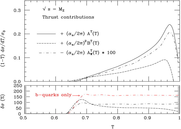
Figure 6: The LO, NLO-QCD and NLO-W contributions to the coefficient functions entering the integrated Thrust distribution, see eq. (14), for process (9) (top) and the relative size of the two NLO corrections (bottom), at $\sqrt{s}=M_{Z}$. The correction for the case of $b$-quarks only is also presented, relative to the LO results for process (10). (Notice that the $\sim A_{\mathrm{W}}$ terms have been plotted with opposite sign and multiplied by hundred for better presentation.)

In view of these percent effects being well above the error estimate expected at a future high-luminosity LC running at the $Z$ pole, it is then worthwhile to further consider the effects of NLO-W corrections to some other ‘infrared-safe’ jet observables typically used in the determination of $\alpha_{\mathrm{S}}$, the so-called ‘shape variables’. A representative quantity in this respect is the Thrust (T) distribution. This is defined as the sum of the longitudinal momenta relative to the (Thrust) axis $n_{\rm T}$ chosen to maximise this sum, i.e.:

$$\mbox{T}={\rm max}\frac{\sum_{i}|\vec{p_{i}}\cdot\vec{n_{\mathrm{T}}}|}{\sum_{i}|\vec{p_{i}}|},$$ (13)

where $i$ runs over all final state clusters. This quantity is identically one at Born level, getting the first non-trivial contribution through ${\cal O}(\alpha_{\mathrm{S}})$ from events of the type (9)–(10). Also notice that any other higher order contribution will affect this observable. Through ${\cal O}(\alpha_{\mathrm{S}}^{2})$, for the choice $\mu=\sqrt{s}$ of the renormalisation scale, the T distribution can be parametrised in the following form:

$$(1-{\rm{T}})\frac{d\sigma}{d\mbox{T}}\frac{1}{\sigma_{0}}=\left(\frac{\alpha_{\mathrm{S}}}{2\pi}\right)A^{\mathrm{\tiny T}}(\mbox{T})+\left(\frac{\alpha_{\mathrm{S}}}{2\pi}\right)^{2}B^{\mathrm{\tiny T}}(\mbox{T}).$$ (14)

Again, the replacement

$$A^{\mathrm{\tiny T}}(\mbox{T})\to A^{\mathrm{\tiny T}}(\mbox{T})+A^{\mathrm{\tiny T}}_{\rm{W}}(\mbox{T})$$ (15)

accounts for the inclusion of the NLO-W contributions.

We plot the terms $\left(\frac{\alpha_{\mathrm{S}}}{2\pi}\right)A^{\mathrm{\tiny T}}(\mbox{T})$, $\left(\frac{\alpha_{\mathrm{S}}}{2\pi}\right)A^{\mathrm{\tiny T}}_{\rm{W}}(\mbox{T})$ and $\left(\frac{\alpha_{\mathrm{S}}}{2\pi}\right)^{2}B^{\mathrm{\tiny T}}(\mbox{T})$ in Fig. 6, always at $\sqrt{s}=M_{Z}$, alongside the relative rates of the NLO-QCD and NLO-W terms with respect to the LO contribution. Here, it can be seen that the NLO-W effects can reach the level of $-1\%$ or so and that they are fairly constant for $0.7\>\raisebox{-2.15277pt}{$\stackrel{{\scriptstyle\textstyle<}}{{\sim}}$}\>{\rm{T}}\>\raisebox{-2.15277pt}{$\stackrel{{\scriptstyle\textstyle<}}{{\sim}}$}\>1$. For the case of $b$-quarks only, similarly to what seen already for the inclusive rates, the NLO-W corrections are larger, as they can reach the $-1.6\%$ level.

3.2 $Z$/$\gamma$ Hadroproduction at Finite Transverse Momentum[22]

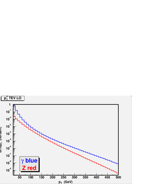
Figure 7: The transverse momentum dependence of the $\gamma$- and $Z$-boson cross sections in (16) at LO (top frame) and the size of the one-loop weak corrections (bottom frame), at Tevatron ($\sqrt{s}_{p\bar{p}}=2$ TeV). Notice that the pseudorapidity range of the jet in the final state is limited to $|\eta|<3$.

The neutral-current processes ($V=\gamma,Z$)

$$q\bar{q}\to gV\quad{\rm{and}}\quad q(\bar{q})g\to q(\bar{q})V$$ (16)

with $V\to\ell^{+}\ell^{-}$ are two of the cleanest probes of the partonic content of (anti)protons, in particular of antiquark and gluon densities. In order to measure the latter it is necessary to study the vector boson $p_{T}$ spectrum. According to [23, 24] the gluon density dominates for $p_{T}\ >Q/2$ where $Q$ is the lepton pair invariant mass. In the presence of polarised beams these reactions give access to the spin–dependent gluon distribution which is presently only poorly known. Thanks to the introduction of improved algorithms [25]–[27] for the selection of (prompt) photons generated in the hard scatterings (16), as opposed to those generated in the fragmentation of the accompanying gluon/quark jet, and to the high experimental resolution achievable in reconstructing $Z\to\ell^{+}\ell^{-}$ ($\ell=e,\mu$) decays, they are regarded – together with the twin charged-current channels

$$q\bar{q}^{\prime}\to gW\quad{\rm{and}}\quad q(\bar{q})g\to q^{\prime}(\bar{q}^{\prime})W,$$ (17)

wherein $W\to\ell\nu_{\ell}$ – as precision observables in hadronic physics. In fact, in some instances, accuracies of order one percent are expected to be attained in measuring these processes [3], both at present and future proton-(anti)proton experiments. These include the Relativistic Heavy Ion Collider running with polarised proton beams (RHIC-Spin) at BNL ($\sqrt{s}_{pp}=300-600$ GeV), the Tevatron collider at FNAL (Run 2, $\sqrt{s}_{p\bar{p}}=2$ TeV) and the Large Hadron Collider (LHC) at CERN ($\sqrt{s}_{pp}=14$ TeV).

Not surprisingly then, a lot of effort has been spent over the years in computing higher order corrections to all such Drell–Yan type processes. To stay with the neutral-current ones these include next-to-leading order (NLO) QCD calculations of both prompt-photon [28, 29] and vector boson production [30]. QCD corrections to the $p_{T}$ distributions have been computed in Refs. [31, 32]. As for the full $\cal O(\alpha)$ Electro-Weak (EW) corrections to $Z$ production and continuum neutral-current processes (at zero transverse momentum), these have been completed in [33] (see also [34]), building on the calculation of the QED part in [35].

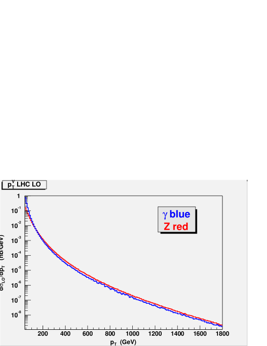
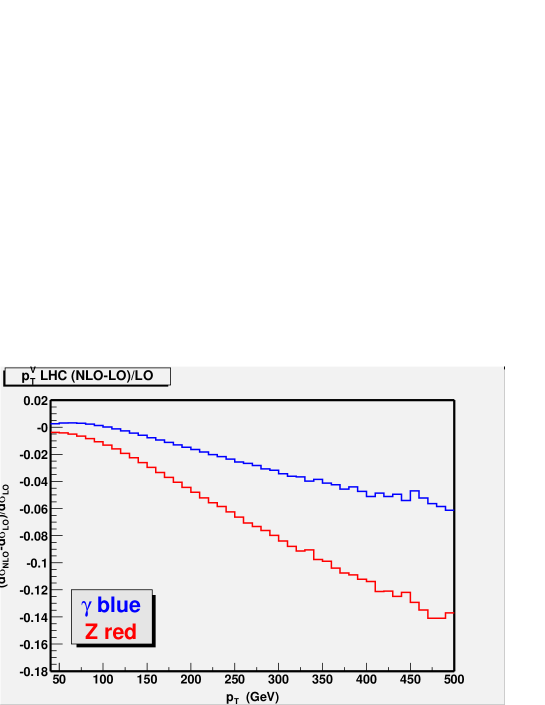
Figure 8: The transverse momentum dependence of the $\gamma$- and $Z$-boson cross sections in (16) at LO (top frame) and the size of the one-loop weak corrections (bottom frame), at LHC ($\sqrt{s}_{pp}=14$ TeV). Notice that the pseudorapidity range of the jet in the final state is limited to $|\eta|<4.5$.

Figs. 7–8 show the effects of the ${\cal O}(\alpha_{\rm{S}}\alpha_{\rm{EW}}^{2})$ terms relatively to the ${\cal O}(\alpha_{\rm{S}}\alpha_{\rm{EW}})$ Born results ($\alpha_{\rm{EM}}$ replaces $\alpha_{\rm{EW}}$ for photons), as well as the absolute magnitude of the latter, as a function of the transverse momentum, at Tevatron and LHC, respectively. The corrections are found to be rather large at both colliders, particularly for $Z$-production. In case of the latter, such effects are of order –7% at Tevatron for $p_{T}\approx 300$ GeV and –14% at LHC for $p_{T}\approx 500$ GeV. In general, above $p_{T}\approx 100$ GeV, they tend to (negatively) increase, more or less linearly, with $p_{T}$. Such effects will be hard to observe at Tevatron but will indeed be observable at LHC. For example, at FNAL, for $Z$-production and decay into electrons and muons with BR$(Z\rightarrow e,\mu)\approx 6.5\%$, assuming $L=2-20$ fb^-1 as integrated luminosity, in a window of 10 GeV at $p_{T}=100$ GeV, one finds 500–5000 $Z+j$ events at LO, hence a $\delta\sigma/\sigma\approx-1.2\%$ EW NLO correction corresponds to only 6–60 fewer events. At CERN, for the same production and decay channel, assuming now $L=30$ fb^-1, in a window of 40 GeV at $p_{T}=450$ GeV, we expect about 2000 $Z+j$ events from LO, so that a $\delta\sigma/\sigma\approx-12\%$ EW NLO correction corresponds to 240 fewer events. In line with the normalisations seen in the top frames of Figs. 7–8 and the size of the corrections in the bottom ones, absolute rates for the photon are similar to those for the massive gauge boson while ${\cal O}(\alpha_{\rm{S}}\alpha_{\rm{EW}}^{2})$ corrections are about a factor of two smaller.

3.3 $b\overline{b}$ Production at TeV Energy Hadron Colliders[4]

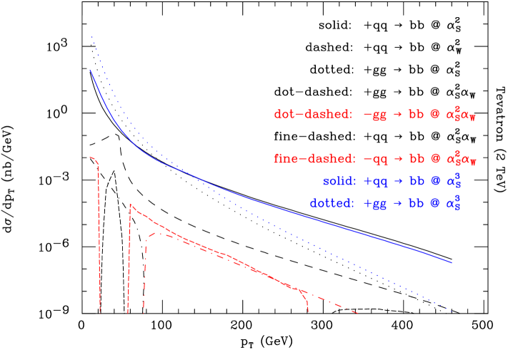
Figure 9: The total cross section contributions vs. the transverse momentum of the $b$-jet for $p\bar{p}\to b\bar{b}$ production at Tevatron (2 TeV) as obtained via the various subprocesses discussed in the text (top) and the corrections due to the $\alpha_{\rm{EW}}^{2}$, $\alpha_{\rm{S}}^{2}\alpha_{\rm{EW}}^{2}$ and $\alpha_{\rm{S}}^{3}$ terms relative to the $\alpha_{\rm{S}}^{2}$ ones (bottom).

Figure 10: The forward-backward asymmetry vs. the transverse momentum of the $b$-jet for $p\bar{p}\to b\bar{b}$ events at Tevatron (2 TeV), as obtained at tree-level and one-loop order (top) and the relative correction of the latter to the former (bottom). (Errors in the ratio are statistical.)

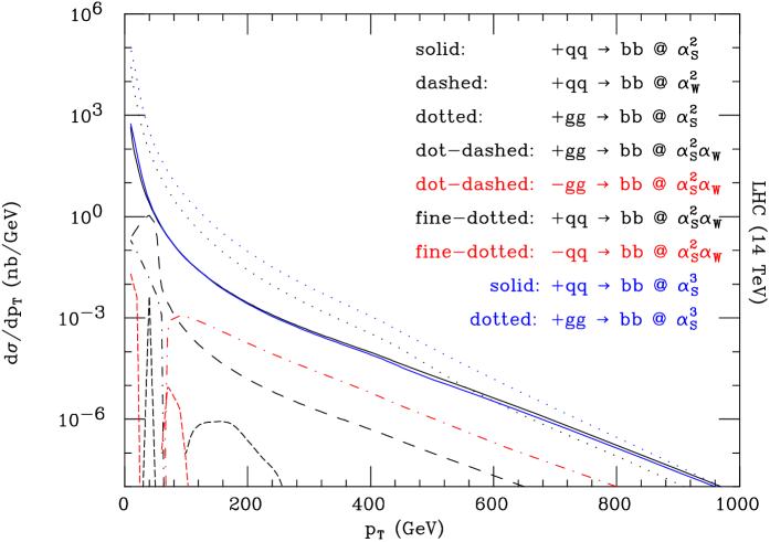
Figure 11: The total cross section contributions vs. the transverse momentum of the $b$-jet for $pp\to b\bar{b}$ production at LHC (14 TeV) as obtained via the various subprocesses discussed in the text (top) and the corrections due to the $\alpha_{\rm{EW}}^{2}$ and $\alpha_{\rm{S}}^{2}\alpha_{\rm{EW}}^{2}$ terms relative to the $\alpha_{\rm{S}}^{2}$ ones (bottom). (Here, we do not show the corrections due to $\alpha_{\rm{S}}^{3}$ terms as results are perturbatively unreliable, given that $K$-factors as large as 3–4 can appear.)

The inclusive $b$-jet cross section at both Tevatron and LHC is dominated by the pure QCD contributions $gg\to b\bar{b}$ and $q\bar{q}\to b\bar{b}$, known through order $\alpha_{\rm S}^{n}$ for $n=2,3$. Of particular relevance in this context is the fact that for the flavour creation mechanisms no $\alpha_{\rm S}\alpha_{\rm{W}}$ tree-level contributions are allowed, because of colour conservation: i.e.,

(18)

where the wavy line represents a $Z$ boson (or a photon) and the helical one a gluon. Tree-level asymmetric terms through the order $\alpha_{\rm{EW}}^{2}$ are however finite, as they are given by non-zero quark-antiquark initiated diagrams such as the one above wherein the gluon is replaced by a $Z$ boson (or a photon). The latter are the leading contribution to the forward-backward asymmetry (more precisely, those graphs containing one or two $Z$ bosons are, as those involving two photons are subleading in this case, even with respect to the pure QCD contributions).

We have computed one-loop and (gluon) radiative contributions through the order $\alpha_{\rm S}^{2}\alpha_{\rm{W}}$, which – in the case of quark-antiquark induced subprocesses – are represented schematically by the following diagrams:

+ all self-energies +

(19)

The gluon bremsstrahlung graphs are needed in order to cancel the infinities arising in the virtual contributions when the intermediate gluon becomes infrared. Furthermore, one also has to include $\alpha_{\rm S}^{2}\alpha_{\rm{W}}$ terms induced by gluon-gluon scattering, that is, interferences between the graphs displayed in Fig. 1 of Ref. [7] and the tree-level ones for $gg\to b\bar{b}$.

The total cross section, $\sigma(p\bar{p}\to b\bar{b})$, for Tevatron (Run2) can be found in Fig. 9 (top), as a function of the transverse momentum of the $b$-jet (or $\bar{b}$-jet) and decomposed in terms of the various subprocesses discussed so far. (Hereafter, the pseudorapidity is limited between $-2$ and $2$ in the partonic CM frame.) The dominance at inclusive level of the pure QCD contributions is manifest, over the entire $p_{T}$ spectrum. At low transverse momentum it is the gluon-gluon induced subprocess that dominates, with the quark-antiquark one becoming the strongest one at large $p_{T}$. The QCD $K$-factors, defined as the ratio of the $\alpha_{\rm{S}}^{3}$ rates to the $\alpha_{\rm{S}}^{2}$ ones are rather large, of order 2 and positive for the $gg\to b\bar{b}$ subprocess and somewhat smaller for the $q\bar{q}\to b\bar{b}$ case, which has a $p_{T}$-dependent sign. The tree-level $\alpha_{\rm{EW}}^{2}$ terms are much smaller than the QCD rates, typically by three orders of magnitude, with the exception of the $p_{T}\approx M_{Z}/2$ region, where one can appreciate the onset of the $Z$ resonance in $s$-channel. All above terms are positive. The $\alpha_{\rm{S}}^{2}\alpha_{\rm{EW}}$ subprocesses display a more complicated structure, as their sign can change over the transverse momentum spectrum considered, and the behaviour is different in $q\bar{q}\to b\bar{b}(g)$ from $gg\to b\bar{b}$. Overall, the rates for the $\alpha_{\rm{S}}^{2}\alpha_{\rm{EW}}$ channels are smaller by a factor of four or so, compared to the tree-level $\alpha_{\rm{EW}}^{2}$ cross sections. Fig. 9 (bottom) shows the percentage contributions of the $\alpha_{\rm{S}}^{3}$, $\alpha_{\rm{EW}}^{2}$ and $\alpha_{\rm{S}}^{2}\alpha_{\rm{EW}}$ subprocesses, with respect to the leading $\alpha_{\rm{S}}^{2}$ ones, defined as the ratio of each of the former to the latter. The $\alpha_{\rm{S}}^{2}\alpha_{\rm{EW}}$ terms represent a correction of the order of the fraction of percent to the leading $\alpha_{\rm{S}}^{2}$ terms. Clearly, at inclusive level, the effects of the Sudakov logarithms are not large at Tevatron, this being mainly due to the fact that in the partonic scattering processes the hard scale involved is not much larger than the $W$ and $Z$ masses.

Next, we study the forward-backward asymmetry, defined as follows:

$$A_{\rm{FB}}=\frac{\sigma_{+}(p\bar{p}\to b\bar{b})-\sigma_{-}(p\bar{p}\to b\bar{b})}{\sigma_{+}(p\bar{p}\to b\bar{b})+\sigma_{-}(p\bar{p}\to b\bar{b})},$$ (20)

where the subscript $+(-)$ identifies events in which the $b$-jet is produced with polar angle larger(smaller) than 90 degrees respect to one of the two beam directions (hereafter, we use the proton beam as positive $z$-axis). The polar angle is defined in the CM frame of the hard partonic scattering. Notice that we do not implement a jet algorithm, as we integrate over the entire phase space available to the gluon. In practice, this corresponds to summing over the two- and three-jet contributions that one would extract from the application of a jet definition. The solid curve in Fig. 10 (top) represents the sum of the tree-level contributions only, that is, those of order $\alpha_{\rm{S}}^{2}$ and $\alpha_{\rm{EW}}^{2}$, whereas the dashed one also includes the higher-order ones $\alpha_{\rm{S}}^{3}$ and $\alpha_{\rm{S}}^{2}\alpha_{\rm{EW}}$.

The effects of the one-loop weak corrections on this observable are extremely large, as they are not only competitive with, if not larger than, the tree-level weak contributions, but also of opposite sign over most of the considered $p_{T}$ spectrum. They are indeed comparable to the effects through order $\alpha_{\rm{S}}^{3}$ [37]. In absolute terms, the asymmetry is of order $-4\%$ at the $W$, $Z$ resonance and fractions of percent elsewhere, hence it should comfortably be measurable after the end of Run 2.

Fig. 11 shows the same quantities as in Fig. 9, now defined at LHC energy. By a comparative reading, one may appreciate the following aspects. Firstly, the effects at LHC of the $\alpha_{\rm{S}}^{2}\alpha_{\rm{EW}}$ corrections are much larger than the $\alpha_{\rm{EW}}^{2}$ ones already at inclusive level (see top of Fig. 11), as their absolute magnitude becomes of order $-2\%$ or so at large transverse momentum (see bottom of Fig. 11): clearly, logarithmic enhancements are at LHC much more effective than at Tevatron energy scales.

4 Conclusions

Altogether, the results presented here point to the relevance of one-loop ${\cal O}(\alpha_{\rm{W}})$ weak corrections for precision analyses of three-jet rates at future high-luminosity LCs running at the $Z$ pole, such as GigaZ, of prompt-photon and neutral Drell-Yan events at both Tevatron and LHC and of $b$-quark asymmetries (e.g., we have studied the forward-backward one) at Tevatron. (A suitable definition of the $b$-quark forward-backward asymmetry – see, e.g., Ref. [38] – may in fact reveal even larger effects at the LHC.)

References

- [1] M. Melles, Phys. Rept. 375 (2003) 219.
- [2] A. Denner, Talk given at International Europhysics Conference on High-Energy Physics (HEP 2001), Budapest, Hungary, 12-18 Jul 2001. Published in *Budapest 2001, High energy physics* hep2001/129, [hep-ph/0110155].
- [3] G. Bunce, N. Saito, J. Soffer and W. Vogelsang, Ann. Rev. Nucl. Part. Sci. 50 (2000) 525; U. Baur, R.K. Ellis and D. Zeppenfeld, FERMILAB-PUB-00-297 Prepared for Physics at Run II: QCD and Weak Boson Physics Workshop: Final General Meeting, Batavia, Illinois, 4-6 Nov 1999; G. Altarelli and M.L. Mangano (eds.), Proceedings of the Workshop on “Standard Model Physics (and More) at the LHC”, Geneva 2000, CERN 2000-004, 9 May 2000.
- [4] E. Maina, S. Moretti, M.R. Nolten and D.A. Ross, Phys. Lett. B570 (2003) 205, [hep-ph/0401093].
- [5] M. Dittmar, A.S. Nicollerat and A. Djouadi, Phys. Lett. B583 (2004) 111, [hep-ph/0307020] (and references therein).
- [6] C. Bourrely, J.P. Guillet and J. Soffer, Nucl. Phys. B361 (1991) 72.
- [7] J.R. Ellis, S. Moretti and D.A. Ross, J. High Energy Phys. 0106 (2001) 043.
- [8] P. Taxil and J.M. Virey, Phys. Lett. B404 (1997) 302.
- [9] P. Taxil and J.M. Virey, Phys. Rev. D55 (1997) 4480.
- [10] P. Taxil and J.M. Virey, Phys. Lett. B441 (1998) 376.
- [11] P. Taxil and J.M. Virey, Phys. Lett. B383 (1996) 355.
- [12] G. Passarino and M.J.G. Veltman, Nucl. Phys. B160 (1979) 151.
- [13] J.A.M. Vermaseren, preprint NIKHEF-00-032 [math-ph/0010025].
- [14] J. Küblbeck, M. Böhm and A. Denner, Comput. Phys. Commun. 64 (1991) 165.
- [15] G.J. van Oldenborgh, Comput. Phys. Commun. 66 (1991) 1.
- [16] E. Maina, S. Moretti and D.A. Ross, J. High Energy Phys. 0304 (2003) 056.
-
[17]
See, e.g.:
M. Consoli and W. Hollik (conveners), in proceedings of the workshop ‘ Physics at LEP1’ (G. Altarelli, R. Kleiss and C. Verzegnassi, eds.), preprint CERN-89-08, 21 September 1989 (and references therein). - [18] V.A. Khoze, D.J. Miller, S. Moretti and W.J. Stirling, J. High Energy Phys. 07 (1999) 014.
- [19] W. Beenakker and A. Werthenbach, Phys. Lett. B489 (2000) 148 [hep-ph/0005316].
- [20] G. Dissertori, talk presented at the ‘XXXI International Conference on High Energy Physics’, Amsterdam, 24-31 July 2002, [hep-ex/0209070] (and reference therein).
- [21] M. Winter, LC Note LC-PHSM-2001-016, February 2001 (and references therein).
- [22] E. Maina, S. Moretti and D.A. Ross, [hep-ph/0403050]. To be published in Phys. Lett. B.
- [23] E.L. Berger, L.E. Gordon and M. Klasen, Phys. Rev. D58 (1998) 074012.
- [24] E.L. Berger, L.E. Gordon and M. Klasen, Phys. Rev. D62 (2000) 014014.
- [25] S. Frixione, Phys. Lett. B429 (1998) 369.
- [26] S. Frixione and W. Vogelsang, Nucl. Phys. B568 (2000) 60.
- [27] S. Frixione, Nucl. Phys. Proc. Suppl. 79 (1999) 608.
- [28] A.P. Contogouris, B. Kamal, Z. Merebashvili and F.V. Tkachov, Phys. Lett. B304 (1993) 329; Phys. Rev. D48 (1993) 4092; Erratum-ibid.D54 (1996) 7081.
- [29] L.E. Gordon and W. Vogelsang, Phys. Rev. D48 (1993) 3136; ibid. D49 (1994) 170.
- [30] B. Kamal, Phys. Rev. D53 (1996) 1142; ibid. D57 (1998) 6663.
- [31] R.K. Ellis, G. Martinelli and R. Petronzio, Nucl. Phys. B211 (1983) 106.
- [32] B. Arnold and M.H. Reno, Nucl. Phys. B319 (1989) 37; Erratum-ibid. B330 (1990) 284; R.J. Gonsalves, J. Pawlowski and C-F. Wai, Phys. Rev. D40 (1989) 2245.
- [33] U. Baur, O. Brein, W. Hollik, C. Schappacher and D. Wackeroth, Phys. Rev. D65 (2002) 033007.
- [34] S. Haywood et al., Talk given at CERN Workshop on Standard Model Physics (and more) at the LHC (Final Plenary Meeting), Geneva, Switzerland, 14-15 Oct 1999. In *Geneva 1999, Standard model physics (and more) at the LHC* 117-230, [hep-ph/0003275].
- [35] U. Baur, S. Keller and W.K. Sakumoto, Phys. Rev. D57 (1998) 199.
- [36] M. Glück, E. Reya and A. Vogt, Z. Phys. C67, 433 (1995).
- [37] J.H. Kuhn and G. Rodrigo, Phys. Rev. D 59 (1999) 054017, [hep-ph/9807420].; Phys. Rev. Lett. 81 (1998) 49 [hep-ph/9802268].
- [38] M. Dittmar, Phys. Rev. D55 (1997) 161.