KEK-CP-153

LAPTH-1049

TMCP-04-3

Electroweak corrections to Higgs production through $ZZ$ fusion at the linear collider

F. Boudjema¹⁾, J. Fujimoto²⁾, T. Ishikawa²⁾,

T. Kaneko²⁾, K. Kato³⁾, Y. Kurihara²⁾, Y. Shimizu²⁾ and Y. Yasui⁴⁾

1) LAPTH${\;}^{\dagger}$, B.P.110, Annecy-le-Vieux F-74941, France.

2) KEK, Oho 1-1, Tsukuba, Ibaraki 305–0801, Japan.

3) Kogakuin University, Nishi-Shinjuku 1-24, Shinjuku, Tokyo 163–8677, Japan.

4) Tokyo Management College, Ichikawa, Chiba,272-0001,Japan.

^†URA 14-36 du CNRS, associée à l’Université de Savoie.

1 Introduction

The hunt for the Higgs and the elucidation of the mechanism of symmetry breaking is the primary task of all future colliders. While the discovery of the Standard Model Higgs at the LHC has been established for a wide range of Higgs masses, only rough estimates on its properties will be possible, through measurements on the couplings of the Higgs to fermions and gauge bosons[1] for example. Precise extraction of these parameters will have to await the advent of the Linear Collider, LC, [2, 3, 4]. Moreover for these measurements to be confronted with theory, calculations beyond tree-level are mandatory. Nonetheless, although the branching ratios of the Higgs have, for some time now, been computed with great precision it is only during the last year that the one-loop electroweak radiative corrections to the main production channel at the LC, $e^{+}e^{-}\rightarrow\nu\bar{\nu}H$, has been achieved[5, 6, 7]. This is because this process is a challenging $3$-body final state and was the first example of its class to have received a full one-loop treatment.

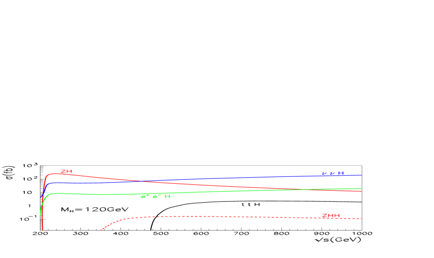
Figure 1: Total cross section for the main Higgs production channels at the linear collider.

As Fig. 1 shows, at the LC energies, $e^{+}e^{-}\rightarrow\nu\bar{\nu}H\;$by far exceeds the yield of the oft-discussed two body process $e^{+}e^{-}\rightarrow ZH\;$. This is especially the case for Higgs masses in accord with the latest indirect precision data[8] that point towards a rather light Higgs with a mass not much greater than the $W$ pair threshold. This is also within the range predicted for the lightest Higgs of the minimal supersymmetric model(MSSM). In this mass range at the LC, Fig. 1 also makes evident that the process $e^{+}e^{-}\rightarrow e^{+}e^{-}H\;$is a welcome addition with a cross section in excess of the yield given by $ZH$ production around $1$TeV. It is also important to point out, that especially at TeV energies, because the final electrons tend to be lost in the beam pipe this reaction will have the same signature as the single Higgs production in the $WW$ process so that in effect one needs a precise determination of single Higgs production. On the other hand, forcing the electrons to be observable, this reaction can be used in improving the determination of the $ZZH$ coupling[9]. The aim of this letter is to report on a full ${\cal O}(\alpha)\;$calculation of this process which has been missing so far thus completing a precise knowledge of the full Higgs production profile at the LC. The other production mechanisms shown in Fig. 1, $e^{+}e^{-}\rightarrow t\bar{t}H$ which is crucial for the extraction of the important $t\bar{t}H$ vertex, has been recently computed at one-loop level [10, 11, 12]. Even more recent, is the full ${\cal O}(\alpha)\;$calculation of $e^{+}e^{-}\rightarrow ZHH\;$[13, 14] which is important for the reconstruction of the Higgs potential through the measurement of the $HHH$ vertex.

2 Grace-loop and the calculation of $e^{+}e^{-}\rightarrow e^{+}e^{-}H\;$

2.1 Checks on the one-loop result

The calculation of the complete electroweak corrections to the process $e^{+}e^{-}\rightarrow e^{+}e^{-}H\;$is performed with the help of GRACE-loop which is described in detail in[15]. This is a code for the automatic generation and calculation of the full one-loop electroweak radiative corrections in the ${\cal{S}}{\cal{M}}$. The code has successfully reproduced the results of a host of one-loop $2\rightarrow 2$ electroweak processes[15]. During the past year GRACE-loop provided the first results on the full one-loop radiative corrections to $e^{+}e^{-}\rightarrow\nu\bar{\nu}H$ [5, 6] and on $e^{+}e^{-}\rightarrow t\bar{t}H\;$[10] which have now been confirmed by an independent group [7, 11]. The calculation we performed for the process $e^{+}e^{-}\rightarrow ZHH\;$[13] is also in agreement with the calculation of[14]. In GRACE-loop we adopt the on-shell renormalisation scheme according to[6, 15, 16].

For each calculation some stringent consistency checks are performed. The results are verified by performing three kinds of tests at some random points in phase space, that is before full integration on phase space. For these tests to be passed one works in quadruple precision. Details of how these tests are performed are given in[6, 15]. Here we only recall the main features of these tests.

i) We first check the ultraviolet finiteness of the results. This test applies to the whole set of the virtual one-loop diagrams. In order to conduct this test we regularise any infrared divergence by giving the photon a fictitious mass (for this calculation we set this at $\lambda=10^{-21}$GeV). In the intermediate step of the symbolic calculation dealing with loop integrals (in $n$-dimension), we extract the regulator constant $C_{UV}=1/\varepsilon-\gamma_{E}+\log 4\pi$, $n=4-2\varepsilon$, and treat this as a parameter. The ultraviolet finiteness test is performed by varying the dimensional regularisation parameter $C_{UV}$. This parameter could then be set to $0$ in further computation. Quantitatively for the process at hand, the ultraviolet finiteness test gives a result that is stable over $15$ digits when one varies the dimensional regularisation parameter $C_{UV}$.

ii) The test on the infrared finiteness is performed by including both the loop and the soft bremsstrahlung contributions and checking that there is no dependence on the fictitious photon mass $\lambda$. The soft bremsstrahlung part consists of a soft photon contribution where the external photon is required to have an energy $k_{\gamma}^{0}<k_{c}\ll E_{b}$. $E_{b}$ is the beam energy. This part factorises and can be dealt with analytically. For the QED infrared finiteness test we also find results that are stable over $15$ digits when varying the fictitious photon mass $\lambda$.

iii) A crucial test concerns the gauge parameter independence of the results. Gauge parameter independence of the result is performed through a set of five gauge fixing parameters. For the latter a generalised non-linear gauge fixing condition[15] has been chosen,

$${{\cal L}}_{GF} = -\frac{1}{\xi_{W}}|(\partial_{\mu}\;-\;ie\tilde{\alpha}A_{\mu}\;-\;igc_{W}\tilde{\beta}Z_{\mu})W^{\mu+}+\xi_{W}\frac{g}{2}(v+\tilde{\delta}H+i\tilde{\kappa}\chi_{3})\chi^{+}|^{2}$$ (1)

$$\;-\frac{1}{2\xi_{Z}}(\partial.Z+\xi_{Z}\frac{g}{2c_{W}}(v+\tilde{\varepsilon}H)\chi_{3})^{2}\;-\frac{1}{2\xi_{A}}(\partial.A)^{2}\;.$$

The $\chi$ represents the Goldstone. We take the ’t Hooft-Feynman gauge with $\xi_{W}=\xi_{Z}=\xi_{A}=1$ so that no “longitudinal” term in the gauge propagators contributes. Not only this makes the expressions much simpler and avoids unnecessary large cancellations, but it also avoids the need for higher tensor structures in the loop integrals. The use of the five parameters, $\tilde{\alpha},\tilde{\beta},\tilde{\delta},\tilde{\kappa},\tilde{\varepsilon}$ is not redundant as often these parameters check complementary sets of diagrams. Let us also point out that when performing this check we keep the full set of diagrams including couplings of the Goldstone and Higgs to the electron for example, as will be done for the process under consideration. Only at the stage of integrating over the phase space do we switch these negligible contributions off. We should add that for this test we omit all widths. Here, the gauge parameter independence checks give results that are stable over $21$ digits (or better) when varying any of the non-linear gauge fixing parameters.

iv) The tensor reduction, down to the scalar integrals, of all loop integrals of rank $N<5$ is performed in the space of the Feynman parameters as detailed in our review[15]. For the $N=1,2$ scalar integrals we implement full analytical formulae, whereas for the scalar $N=3,4$ integrals we use the FF package[17] supplemented by our own routines for the QED (infrared with photon-exchange) scalar integrals. The treatment of the five-point functions is as detailed in our previous paper on $e^{+}e^{-}\rightarrow ZHH\;$[13].

2.2 Input parameters

The input parameters for the calculation are the same as those we have used for the calculation of $e^{+}e^{-}\rightarrow ZHH$. We recall them here. We take for the fine structure constant in the Thomson limit $\alpha^{-1}=137.0359895$ and $M_{Z}=91.1876$GeV for the $Z$ mass. The on-shell renormalisation program, which we have described in detail elsewhere[15], uses $M_{W}$ as an input. However, the numerical value of $M_{W}$ is derived through $\Delta r$[18] with $G_{\mu}=1.16639\times 10^{-5}{\rm GeV}^{-2}$. Thus, $M_{W}$ changes as a function of $M_{H}$. For the lepton masses we take $m_{e}=0.510999$ MeV, $m_{\mu}=105.658389$ MeV and $m_{\tau}=1.7771$ GeV. For the quark masses, beside the top mass $m_{t}=174$ GeV, we take the set $m_{u}=m_{d}=63$ MeV, $m_{s}=94$ MeV, $m_{c}=1.5$ GeV and $m_{b}=4.7$ GeV. This set of effective quark masses reproduces $\Delta\alpha^{(5)}_{\rm had}(M_{Z}^{2})=276.094\;10^{-4}$ in a (naive) perturbative one-loop calculation of the running $\alpha$ at $M_{Z}$, in excellent agreement with the value used by the Electroweak Working Group[8]. With this we find, for example, that $M_{W}=80.3766$GeV ($\Delta r=2.549\%$) for $M_{H}=120$GeV and $M_{W}=80.3477$GeV ($\Delta r=2.697\%$) for $M_{H}=180$GeV. For this process, as we will discuss shortly we also need to specify the $Z$-width. For this we have used a one-loop formula, which gives $\Gamma_{Z}=2.4945$GeV for $M_{H}=120$GeV and $\Gamma_{Z}=2.4927$GeV for $M_{H}=180$GeV. Both values are in fact within $1\sigma$ of the experimental value $\Gamma_{Z}=2.4956$. The lower bound of the ${\cal{S}}{\cal{M}}\;$Higgs boson mass from LEP2 is 114.4 GeV[19], while the indirect electroweak precision measurement set an upper bound for the ${\cal{S}}{\cal{M}}\;$Higgs mass at about 200 GeV[8]. In this paper, we therefore only consider a relatively light ${\cal{S}}{\cal{M}}\;$Higgs boson and take the illustrative values $M_{H}=120$GeV, $M_{H}=150$GeV and $M_{H}=180$GeV.

3 Tree-level calculation

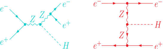
Figure 2: Contributing diagrams at tree-level in terms of the s-channel type, left panel, obtained from $e^{+}e^{-}\rightarrow ZH$, and the $t$-channel type from $ZZ$ fusion.

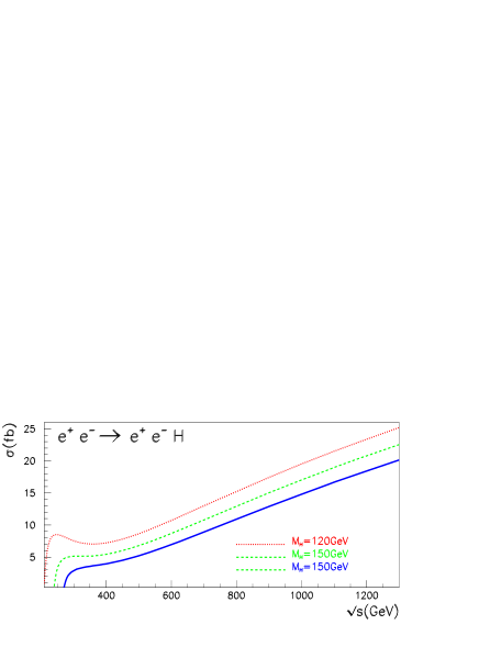
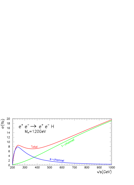
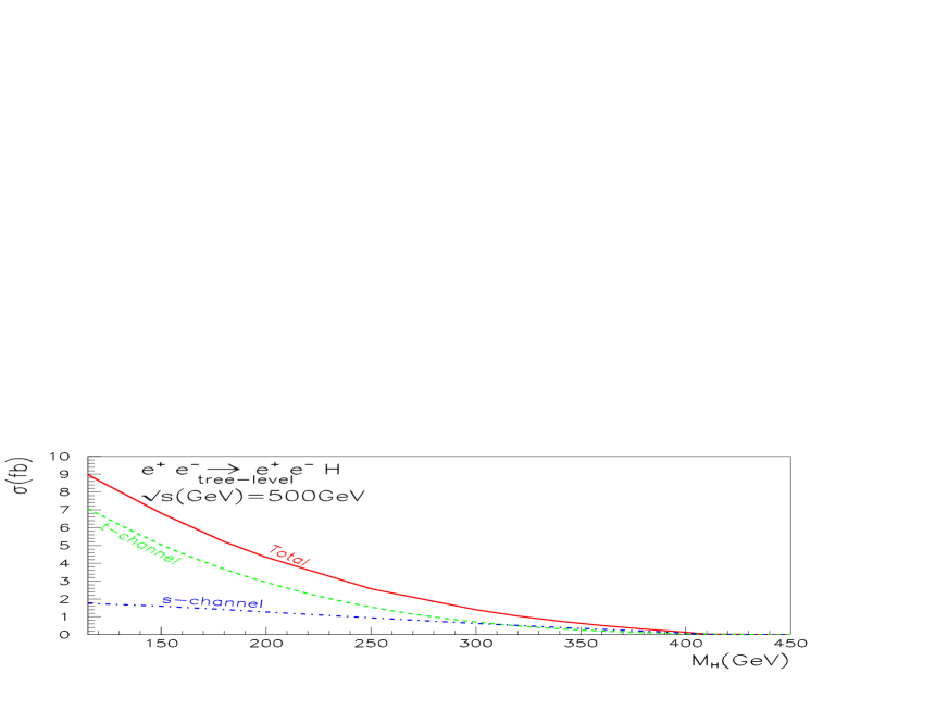
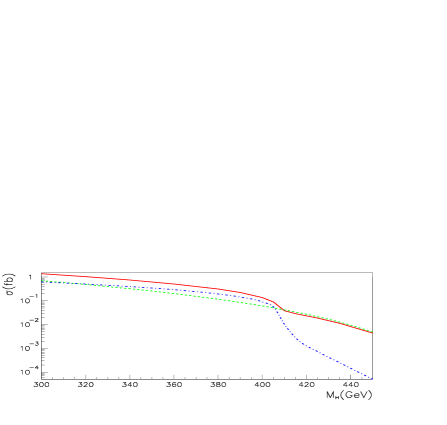
Figure 3: Tree-level cross sections for $e^{+}e^{-}\rightarrow e^{+}e^{-}H\;$. The first panel shows the centre of mass energy dependence for three value of the Higs mass. For $M_{H}=120$GeV, beside the total cross section we show the $s$-channel and $t$-channel contributions. In the panel at the bottom the dependence of the cross section as a function of the Higgs mass is shown at a centre-of-mass $\sqrt{s}=500$GeV.

At tree-level, in the unitary gauge, the $e^{+}e^{-}\rightarrow e^{+}e^{-}H\;$process is built up from $s$-channel diagram originating from $e^{+}e^{-}\rightarrow ZH\;$and a $t$-channel diagram which is a fusion type, see Fig. 2. Each type constitutes, on its own, a gauge independent process. In fact the former (neglecting lepton masses) can be defined as $e^{+}e^{-}\rightarrow\mu^{+}\mu^{-}H$. In principle it is only the $Z$ coupling to the outgoing lepton, in this $s$-channel contribution, which can be resonating and thus requires a finite width. Nonetheless in our code we dress both $Z$ in the $s$-channel type diagrams with a constant $Z$ width. We apply no width to the $Z$ taking part in the $ZZ$-fusion diagrams.
For a light Higgs mass and for the LC energies, past $\sqrt{s}=500$GeV, the cross section is dominated by the $Z$-fusion, which grows (logarithmically) with energy, see Fig. 3. The $s$-channel contribution follows $e^{+}e^{-}\rightarrow ZH\;$very closely, in the order of $10\%$ of the total $e^{+}e^{-}\rightarrow e^{+}e^{-}H\;$at $500$GeV but drops quite fast to amount to a mere $2\%$ at $1$TeV for $M_{H}=120$GeV. With $\sqrt{s}=500$GeV the cross section for $M_{H}=$120GeV is of the order of $10$fb. Although it is about an order of magnitude smaller than single Higgs production $e^{+}e^{-}\rightarrow\nu\bar{\nu}H\;$, this cross section amounts to about $10^{4}$ events with a total integrated luminosity of $1$ab^-1. The $1\sigma$ statistical error corresponds to about $1\%$. Thus the theoretical knowledge of the cross section at $0.1\%$ is quite sufficient. At a moderate LC energy of $\sqrt{s}=500$GeV, the cross section drops rather quickly with increasing Higgs mass, Fig. 3, reaching the order of $1$fb for $M_{H}=300$GeV. This drop is especially dramatic for the $t$-channel, for this Higgs mass at this energy the $s$ and $t$-channel are about equal. The $s$-channel slightly takes over before dropping precipitously at threshold $\sqrt{s}\sim M_{Z}+M_{H}$.

It is also important to note, as this will help understand the QED corrections, the steep increase of the cross section at threshold.

4 Results at one-loop

4.1 Classification and overview of the diagrams

Figure 4: A small selection of different classes of loop diagrams contributing to $e^{+}e^{-}\rightarrow e^{+}e^{-}H\;$. We keep the same graph numbering as that produced by the system. Graph 4311 belongs to the corrections from self-energies, here both the virtual and counterterm contributions are generated and counted as one diagram. Graph 349 shows a vertex correction. Both graphs are considered as $s$-channel resonant Higgs-strahlung contributions. Graph 762 represents a box correction, it is a non resonant contribution, which can not be deduced from $e^{+}e^{-}\rightarrow ZH\;$, but applies also to the correction to the $s$-channel $e^{+}e^{-}\rightarrow\mu^{+}\mu^{-}H$. Graph 1481 is also a box correction counted as a correction to the $ZZ$ fusion. Graph 1575, Graph 1741 and Graph 1757 are fusion type corrections involving $\gamma\gamma$, $Z\gamma$ and $ZZ$ fusion. Graph 2607 shows a pentagon correction which also counts as an $s$-channel since it is induced for $e^{+}e^{-}\rightarrow\mu^{+}\mu^{-}H$. Graph 3157 on the other hand is a pentagon correction that only applies to $e^{+}e^{-}\rightarrow e^{+}e^{-}H\;$.

The full set of the one-loop Feynman diagrams within the non-linear gauge fixing condition consists of as many as $4470$ contributions for the full ${\cal O}(\alpha)$ correction. This is to be compared to $1350$ diagrams for the $e^{+}e^{-}\rightarrow\nu\bar{\nu}H\;$process. A selection of these diagrams is displayed in Fig. 4. These can be brought down to $510$ diagrams (as compared to $249$ for $e^{+}e^{-}\rightarrow\nu\bar{\nu}H\;$) when we neglect the electron Yukawa coupling to the Higgs and the Goldstones. The latter set we refer to as the production set as we use it for the numerical computation of the cross section. The former set is used to conduct the detailed tests of gauge parameter independence and ultra-violet finiteness as described in the previous section. All the one-loop diagrams can still be unambiguously divided into $s$-channel and $t$-channel contribution. The former are the ones one would still obtain in calculating $e^{+}e^{-}\rightarrow\mu^{+}\mu^{-}H$ and obviously constitute a gauge invariant subset.
Of these one-loop diagrams, those corresponding to the pure QED corrections can be easily extracted in a gauge invariant way. They correspond to adding an internal photon between any two external electron lines of the tree-level diagrams of Figs 2. These QED diagrams can therefore be further subdivided into $s$- and $t$-channel contributions. These QED corrections consist then of either pentagons or photonic corrections to the $eeZ$ vertex (with its counterterms).

4.2 Treatment of the $Z$-width at the loop-level

There is no definite, completely general and satisfactory implementation of the width of an unstable gauge particle in loop calculations. Many comparisons with different implementations of the width[20, 21] have been made. Nonetheless it has been found that applying a “constant $Z$ width” is more appropriate than the running width and reproduces the result of much more involved schemes (like the ‘fermion scheme”[20]). For the case at hand, the introduction of a width is required only for the $Z$ coupling to the final electron pair. For this implementation of the width to the $s$-channel neutral gauge boson, various ways should have a negligible effect as has been found for the similar process $e^{+}e^{-}\rightarrow\nu\bar{\nu}H\;$[6, 7]. Moreover the $s$-channel contribution is much smaller than the $t$-channel contributions, in the latter we do not endow the $Z$ propagators with a width. Building up on the implementation of the width at tree-level, we include a constant width to all $Z$ propagators not circulating in a loop for the $s$-channel type diagrams. For example we add a width to all $Z$ in graphs 349,762,4311 of Fig. 4. As will be explained below when discussing QED corrections, the $Z$ propagators inside QED pentagon diagrams of the $s$-channel type are also calculated with the addition of the constant $Z$-width.

For those one-loop diagrams with a self-energy correction to any $Z$ propagator, represented by graph 4311 in Fig. 4, we follow a procedure along the lines described in [22]. We will show how this is done with a single $Z$ exchange coupling to a fermion pair of invariant mass $s_{f\bar{f}}$.
First, it is important to keep in mind, however, that our tree-level calculation of the $s$-channel is done by supplying the width in the $Z$ propagator. Therefore it somehow also includes parts of the higher order corrections to the $Z$ self-energy which should be subtracted when performing a higher order calculation. The case at hand is as simple as consisting, at tree-level, of one single diagram. The simplest way to exhibit this subtraction is to rewrite, the zero-th order amplitude, ${\cal{M}}^{(0)}$, before inclusion of a width, in terms of what we call the tree-level (regularised) amplitude, ${\widetilde{\cal M}}^{{\rm tree}}$

$${\cal{M}}^{(0)}=\frac{{\cal{N}}^{(0)}}{s_{f\bar{f}}-M_{Z}^{2}}=\overbrace{\frac{{\cal{N}}^{(0)}}{s_{f\bar{f}}-M_{Z}^{2}+i\Gamma_{Z}M_{Z}}}^{{\widetilde{\cal M}}^{{\rm tree}}}\left(1+\frac{i(\Gamma_{Z}^{0}+\Delta\Gamma_{Z})M_{Z}}{s_{f\bar{f}}-M_{Z}^{2}}\right),\quad\Delta\Gamma_{Z}=\Gamma_{Z}-\Gamma_{Z}^{0}.$$ (2)

The $\Gamma_{Z}^{0}$ contribution will be combined with the one-loop correction while $\Delta\Gamma_{Z}$ will be counted as being beyond one-loop.

At the one-loop level, before the summation à la Dyson and the inclusion of any “hard” width, the amplitude is gauge-invariant and can be decomposed as

$${\cal{M}}^{(1)} = \frac{{\cal{N}}^{(0)}}{s_{f\bar{f}}-M_{Z}^{2}}\frac{\tilde{\Pi}_{T}^{ZZ}(s_{f\bar{f}})}{s_{f\bar{f}}-M_{Z}^{2}}+\frac{A_{Z\gamma}\frac{\tilde{\Pi}_{T}^{Z\gamma}(s_{f\bar{f}})}{s_{f\bar{f}}}}{s_{f\bar{f}}-M_{Z}^{2}}+\frac{R_{Z}}{s_{f\bar{f}}-M_{Z}^{2}}+C$$ (3)

$$= \frac{1}{s_{f\bar{f}}-M_{Z}^{2}}\left\{{\cal{N}}^{(0)}\frac{\tilde{\Pi}_{T}^{ZZ}(s_{f\bar{f}})}{s_{f\bar{f}}-M_{Z}^{2}}+\left(A_{Z\gamma}\frac{\tilde{\Pi}_{T}^{Z\gamma}(s_{f\bar{f}})}{s_{f\bar{f}}}+R_{Z}\right)+(s_{f\bar{f}}-M_{Z}^{2})C\right\}.$$

The different contributions in ${\cal{M}}^{(1)}$ are the following. The first term proportional to the tree-level contribution is due to the renormalised transverse part of the $Z$ self-energy correction $\tilde{\Pi}_{T}^{ZZ}$, including counterterms. Such a transition is shown in Graph 4311 of Fig. 4. The term proportional to $A_{Z\gamma}\frac{\tilde{\Pi}_{T}^{Z\gamma}(s_{f\bar{f}})}{s_{f\bar{f}}}$ comes from the renormalised transverse part of the $Z$-$\gamma$ self-energy, $\tilde{\Pi}_{T}^{Z\gamma}$, with the photon attaching to the final fermion (this type is absent for neutrinos in $e^{+}e^{-}\rightarrow\nu\bar{\nu}H$). The $R_{Z}$ terms combine one-loop corrections but which nevertheless still exhibit a $Z$-exchange that couples to the final fermions and hence these type of diagrams can be resonant, an example is Graph 349 of Fig. 4. We can write $R_{Z}=Z_{ZH}+V_{Z}^{f}$, where $Z_{ZH}$ corresponds to the part containing the correction to $e^{+}e^{-}\rightarrow Z^{\star}H$, while $V_{Z}^{f}$ contains the corrections to the final $Z_{f\bar{f}}$ vertex. $Z_{ZH}(s_{f\bar{f}}=M_{Z}^{2})$ corresponds to $e^{+}e^{-}\rightarrow ZH$ and is gauge invariant at the pole. The term $C$ contains all the rest which are apparently non-resonant, an example here is Graph 762 of Fig. 4. Both ${\cal{M}}^{(1)}$ and ${\cal{M}}^{(0)}$ are gauge invariant.

Our procedure, in effects, amounts to first regularising the overall propagator in Eq. 3 by the implementation of a constant $Z$ width and then combining the renormalised $Z$ self-energy part in Eq. 3 with the $\Gamma_{Z}^{0}$ part of Eq. 2. Since our on-shell renormalisation procedure is such that $Re\tilde{\Pi}_{T}^{ZZ}(M_{Z}^{2})=0$ and since $\Gamma_{Z}^{0}=-Im\Sigma_{T}^{ZZ}(M_{Z}^{2})$, see [15], our prescription is to write

$${\cal{M}}^{(0)}+{\cal{M}}^{(1)} \rightarrow \overbrace{\frac{{\cal{N}}^{(0)}}{s_{f\bar{f}}-M_{Z}^{2}+i\Gamma_{Z}M_{Z}}}^{{\widetilde{\cal M}}^{{\rm tree}}}+\overbrace{\frac{1}{s_{f\bar{f}}-M_{Z}^{2}+i\Gamma_{Z}M_{Z}}\widetilde{{\cal N}}^{1}}^{{\widetilde{\cal M}}^{{\rm 1-loop}}}$$

$$\widetilde{{\cal N}}^{1} = {\cal{N}}^{(0)}\frac{\left(\tilde{\Pi}_{T}^{ZZ}(s_{f\bar{f}})-\tilde{\Pi}_{T}^{ZZ}(M_{Z}^{2})\right)}{s_{f\bar{f}}-M_{Z}^{2}}+\left(A_{Z\gamma}\frac{\tilde{\Pi}_{T}^{Z\gamma}(s_{f\bar{f}})}{s_{f\bar{f}}}+R_{Z}\right)$$

$$+ (s_{f\bar{f}}-M_{Z}^{2})C.$$

The above prescription is nothing else but the factorisation procedure avoiding double counting. It is gauge invariant but puts the non-resonant terms to zero on resonance. In practice in the automatic code, we supply a constant $Z$ width to all $Z$ not circulating in a loop and by treating the one-loop $ZZ$ self-energy contribution as in Eq. 4.2. Up to terms of order ${\cal{O}}(\Gamma_{Z}\alpha)$ this is equivalent to Eq. 4.2. In particular the contribution of the $C$ term does not vanish on resonance, since its overall factor is unity rather than the factor $(s_{f\bar{f}}-M_{Z}^{2})/(s_{f\bar{f}}-M_{Z}^{2}+i\Gamma_{Z}M_{Z})$ in the original factorisation prescription.

4.3 Extraction of the QED corrections

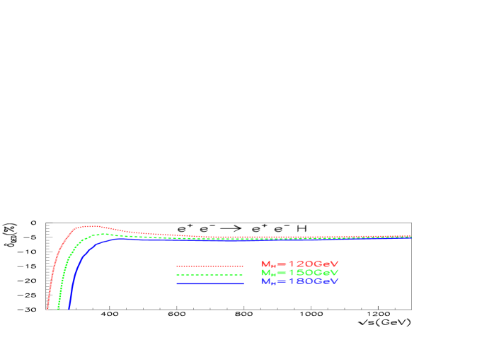
Figure 5: The purely QED corrections as function of the centre of mass energy.

As already discussed, the QED corrections can be isolated unambiguously in this process and separated into those belonging to the $s$- and $t$-channel type corrections because of the simple electric charge flow. For the $t$-channel contribution in $e^{+}e^{-}\rightarrow\nu\bar{\nu}H\;$this was not the case thus preventing an unambiguous extraction of the full QED correction. Only the leading log terms could be identified there. Here, however, a new feature is that now one has both initial state, final state and initial-final state interference QED corrections. The last one in the $s$-channel consists of pentagons. For this class of diagrams the infrared divergence occurs also with the (final) $Z$ being resonant. We thus apply to this internal $Z$ a constant width. This is akin to what occurs for the $Z\gamma$ boxes in $e^{+}e^{-}\rightarrow f\bar{f}$ close to the $Z$ resonance[22]. In fact we recover this feature after the decomposition of the pentagon, where part of this decomposition maps precisely into the scalar $Z\gamma$ box. The $Z$ width is kept consistently in the infrared $Z\gamma$ boxes. For such type of (scalar) boxes we do not rely on the FF package but revert to special routines, see[15, 22]. After inclusion of the bremsstrahlung contribution, this procedure shows that all infrared divergences consistently cancel to a precision reaching $15$ digits when we vary the fictitious photon mass.

The results of the purely QED corrections, including virtual, soft and hard bremmstrahlung are displayed in Fig. 5 for the three Higgs masses $M_{H}=120,150,180$GeV. Around threshold the corrections are large (and negative). For instance for $\sqrt{s}=240$GeV and $M_{H}=120$GeV the total QED correction is about $-13\%$ while for $M_{H}=180$GeV it is about $-17\%$ at $\sqrt{s}=300$GeV. It is to be noticed that the bulk of the contribution for these energies and masses is due to the $s$-channel process which exhibits a very sharp peak at threshold, see Fig. 3. This explains the large negative correction at small energies. This behaviour has been a feature of all $s$-channel processes we have studied so far. As usual these large initial state QED corrections could be resummed through, for example, a structure function approach and QED parton shower, see for instance[23]. Past this energy range, to regions where the $t$-channel contribution dominates and were the cross sections are larger, the QED corrections vary slowly. In fact past about $\sqrt{s}=500$GeV and up $1$TeV, the QED corrections almost flatten out, at $1.3$TeV, they reach about $-5\%$ with little Higgs mass dependence.

4.4 Genuine electroweak corrections

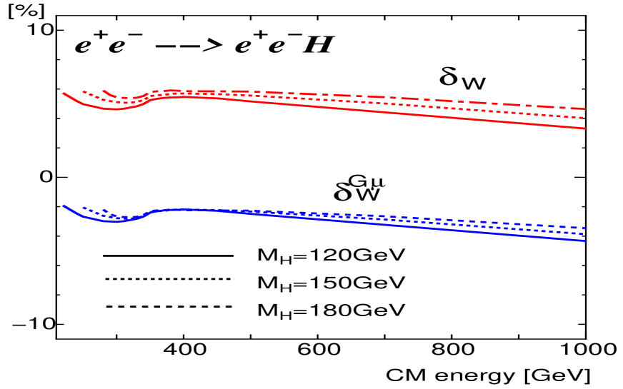
Figure 6: Genuine electroweak correction

The most interesting part of the electroweak corrections consist of the genuine weak corrections which in this process can be unambiguously and easily extracted. Our results are shown in Fig. 6 for the $3$ illustrative Higgs masses, $M_{H}=120,150,180$GeV. In the $\alpha(0)$ scheme, the genuine weak corrections for the entire process are positive. For small energies just above threshold, one notices a feature we have pointed out in our previous calculations[6, 10, 13] and that we termed as the spoon-like behaviour. This behaviour is inherited from the $e^{+}e^{-}\rightarrow ZH\;$process. The corrections show a very slight dependence on the Higgs mass and very slowly decrease with the center-of-mass energy, on the whole they are of order $\sim 5\%$. We have not attempted to extract the corrections for the $s$-channel contribution as the latter follows the one we conducted for the $s$-channel contribution to $e^{+}e^{-}\rightarrow\nu\bar{\nu}H\;$. Moreover at the energies with largest cross sections, the most important contribution is that of the $t$-channel. It is also possible to extract part of the potentially large correction of order $m_{t}^{2}$, as well as the logarithmic correction from small fermion masses in the running of $\alpha$, by reverting to the $G_{\mu}$ scheme. In the latter we simply trade $\alpha$ by $G_{\mu}$. This procedure applied to this $2\rightarrow 3$ process absorbs $3\Delta r$. The genuine electroweak corrections for the entire process in the $G_{\mu}$ scheme are, in absolute terms, even smaller dropping from about $-2\%$ at small energies to about $-4\%$ at $1$TeV, with again very little dependence in the Higgs mass.

It is interesting to compare the genuine weak correction for this process with the weak corrections we found for $e^{+}e^{-}\rightarrow\nu\bar{\nu}H\;$[6]. This is most appropriately done in the $G_{\mu}$ scheme since in [6] our input for the light quarks was slightly different. One finds that the weak corrections are almost of the same order in the two processes for the same Higgs mass and the same energy. For instance for $M_{H}=150$GeV and $\sqrt{s}=500$GeV, we find $\delta_{W}^{G}=-2.3\%$ in $e^{+}e^{-}\rightarrow e^{+}e^{-}H\;$compared to $\delta_{W}^{G}=-2.2\%$ in $e^{+}e^{-}\rightarrow\nu\bar{\nu}H\;$. At the same energy for $M_{H}=180$GeV we find $\delta_{W}^{G}=-2.3\%$ in $e^{+}e^{-}\rightarrow e^{+}e^{-}H\;$compared to $\delta_{W}^{G}=-1.9\%$ in $e^{+}e^{-}\rightarrow\nu\bar{\nu}H\;$. One should however exercise some caution when interpreting this result which suggests that the radiative corrections in the $G_{\mu}$ scheme in the two processes are about equal. For example, corrections in both channels contain other $m_{t}^{2}$ dependence that are not solely contained in $\Delta r$. These additional heavy $m_{t}^{2}$ corrections that could be subtracted to arrive at an improved approximation are different for the two processes. First of all as we had shown in [6] the genuine weak correction to the $s$-channel contribution is rather large and can not be approximated by subtracting these additional $m_{t}^{2}$ terms, in the heavy top mass limit. On the other hand since at high energy the contribution of the $s$-channel is negligible it is sensible to only parameterise the corrections to the dominant $t$-channel. In $e^{+}e^{-}\rightarrow\nu\bar{\nu}H\;$these heavy top mass $m_{t}^{2}$ terms originate from the $HWW$ vertex. Subtraction of these extra $m_{t}^{2}$ corrections defines, for the dominant $t$-channel processes, an improved approximation[24, 7]

$$\delta_{W,\nu\bar{\nu}H}^{imp}\sim\delta_{W}^{G}+5X_{t}\quad{\rm with}\quad X_{t}=\frac{\alpha}{16\pi}\frac{1}{s_{W}^{2}}\frac{m_{t}^{2}}{M_{W}^{2}}.$$ (5)

For the $e^{+}e^{-}H$ process the extra heavy mass $m_{t}^{2}$ dependence comes from both the $ZHH$ vertex, with the same strength as in the $WWH$ vertex, but also from the $Zf\bar{f}$ vertex as occurs in $Z\rightarrow f\bar{f}$. Moreover this $m_{t}^{2}$ dependence is helicity dependent.

Let us recall that for the $ZZ$ fusion diagrams, the helicity amplitudes that contribute are those of the type $e^{-}_{\lambda}e^{+}_{\lambda^{\prime}}\rightarrow e^{-}_{\lambda}e^{+}_{\lambda^{\prime}}$, neglecting the electron mass. To make the notation simpler we will write the helicity of the positron to correspond to the chirality that represents its corresponding spinor. Pulling out the overall left and right couplings $g_{\lambda}=g_{L,R}$, $g_{L,R}=(-1+2s_{W}^{2},2s_{W}^{2})/(2s_{W}c_{W})$ where $c_{W}=M_{W}/M_{Z}$ and $s_{W}^{2}=1-c_{W}^{2}$, we write the tree-level amplitudes as

$${\cal M}^{ZZ}_{\lambda,\lambda^{\prime}}=e^{2}g_{\lambda}g_{\lambda^{\prime}}\;{\cal N}^{ZZ}_{\lambda,\lambda^{\prime}}$$ (6)

The $m_{t}^{2}$ correction in the $G_{\mu}$ scheme to the helicity amplitude writes as

$${\cal\delta M}^{ZZ}_{\lambda,\lambda^{\prime}}={\cal M}^{ZZ}_{\lambda,\lambda^{\prime}}\times\delta^{G,t}_{W,\{\lambda,\lambda^{\prime}\}};\quad\delta^{G,t}_{W,\{\lambda,\lambda^{\prime}\}}=\frac{X_{t}}{2}\;\left(1+\frac{6c_{W}}{s_{W}}\left(g_{\lambda}^{-1}+g_{\lambda^{\prime}}^{-1}\right)\right)$$ (7)

At high energy the main contribution is from the $t$-channel where both $Z$ are quasi on-shell. One expects, at high energy, that the leading contribution is the same for all amplitudes ${\cal N}^{ZZ}_{\lambda,\lambda^{\prime}}$. In this approximation, the correction to the unpolarized cross section writes as

$$\delta^{G,t}_{W}=X_{t}\;\left(1+12\frac{c_{W}}{s_{W}}\frac{g_{L}+g_{R}}{g_{L}^{2}+g_{R}^{2}}\right)=X_{t}\;\left(1-48c_{W}^{2}\left(\frac{1-4s_{W}^{2}}{1+(1-4s_{W}^{2})^{2}}\right)\right)$$ (8)

The improved approximation for $e^{+}e^{-}\rightarrow e^{+}e^{-}H\;$total cross section would then write

$$\delta_{W,e^{+}e^{-}H}^{imp} \sim \delta_{W}^{G}-\delta^{G,t}_{W}$$ (9)

$\sqrt{s}=500GeV$	$e^{+}e^{-}\rightarrow\nu\bar{\nu}H\;$		$e^{+}e^{-}\rightarrow e^{+}e^{-}H\;$
$M_{H}$(GeV)	$\delta_{W}^{G}(\%)$	$\delta_{W}^{imp}(\%)$	$\delta_{W}^{G}(\%)$	$\delta_{W}^{imp}(\%)$
120	-2.3	-0.8	-2.5	-1.6
150	-2.2	-0.7	-2.3	-1.4
180	-1.9	-0.4	-2.3	-1.4
$\sqrt{s}=1$TeV
$M_{H}=150$GeV	-3.6	-2.1	-3.9	-3.0

Table 1: Comparing the genuine weak corrections in the $G_{\mu}$ scheme and after subtraction of $m_{t}^{2}$ terms between $e^{+}e^{-}\rightarrow\nu\bar{\nu}H\;$and $e^{+}e^{-}\rightarrow e^{+}e^{-}H\;$.

We see, Table 1, that the corrections for the two-processes are within $1\%$ of each other in the improved approximation, both for a centre of mass energy of $500$GeV and $1TeV$ after subtracting the $m_{t}^{2}$ corrections. It is also important to remark that for the $e^{+}e^{-}H$ process the full QED corrections have been subtracted to define the genuine weak corrections whereas for the neutrino process only the universal QED corrections have been subtracted in [6]. This could be another reason for the fortuitous agreement between the weak corrections expressed in the $G_{\mu}$ scheme for the two processes. It is also interesting to note that especially for the $e^{+}e^{-}\rightarrow\nu\bar{\nu}H\;$process the correction in the improved approximation for the light Higgs masses we have studied is quite below $1\%$ at $500$GeV. It is about $2\%$ at 1TeV. We note that the large $m_{t}^{2}$ approximation works better when the top mass is much heavier than all other scales in the problem. Though this is really not the case compared to $M_{W},M_{Z}$ and $M_{H}$, it is still a relatively good approximation. We have however checked explicitly, within the GRACE system, that the approximation works much better with higher Higgs masses $m_{t}^{2}\gg 174$GeV, while the accuracy of the approximation is less clear in the energy range of the LC with $m_{t}^{2}\ll s$. In any case, we should stress that considering the accuracy with which the single Higgs cross sections will be measured, our calculations of $e^{+}e^{-}\rightarrow e^{+}e^{-}H\;$and $e^{+}e^{-}\rightarrow\nu\bar{\nu}H\;$show that one still needs to perform the full electroweak corrections for a precision measurement of the cross section.

5 Conclusions

With the process $e^{+}e^{-}\rightarrow e^{+}e^{-}H\;$we now have complete one-loop prediction for the most dominant processes for Higgs production at the linear collider. Considering that one of the primary aims of this machine is a precise determination of the properties of the Higgs, such calculations have for long been missing. For this process, we have found that the genuine weak corrections when in expressed in the $G_{\mu}$ scheme are quite moderate being of order $-2$ to $-4$% for the Higgs masses preferred by the present indirect limits. The QED corrections in the energy region of LC is quite modest, though it can be quite large at energies around the threshold of production, where the cross sections are small anyhow.

Acknowledgments
This work is part of a collaboration between the GRACE project in the Minami-Tateya group and LAPTH. We gratefully acknowledge the participation of Geneviève Bélanger throughout this project and would like to thank her for her help and comments. We would also like to thank Denis Perret-Gallix for his continuous interest and encouragement. This work was supported in part by the Japan Society for Promotion of Science under the Grant-in-Aid for scientific Research B(N^o 14340081) and PICS-GDRI 397 of the French National Centre for Scientific Research (CNRS). We also thank IDRIS, Institut du Dévelopement et des Resources en Informatique Scientifique for the use of their computing resources (Project N^o 041716).

References

- [1] Precision Higgs Working Group of Snowmass 2001, J. Conway et al., FERMILAB-CONF-01-442, SNOWMASS-2001-P1WG2, Mar 2002. 20pp. Contributed to APS/DPF/DPB Summer Study on the Future of Particle Physics (Snowmass 2001), Snowmass, Colorado, 30 Jun - 21 Jul 2001;hep-ph/0203206.
- [2] T. Abe et al. [American Linear Collider Working Group Collaboration], “Linear collider physics resource book for Snowmass 2001,” in Proc. of the APS/DPF/DPB Summer Study on the Future of Particle Physics (Snowmass 2001) ; hep-ex/106055, hep-ex/106057, hep-ex/106058.
- [3] J. A. Aguilar-Saavedra et al. [ECFA/DESY LC Physics Working Group Collaboration], “TESLA Technical Design Report Part III: Physics at an e+e- Linear Collider,” arXiv:hep-ph/0106315.
- [4] K. Abe et al. [ACFA Linear Collider Working Group Collaboration], “Particle physics experiments at JLC,” arXiv:hep-ph/0109166.
- [5] G. Bélanger, F. Boudjema, J. Fujimoto, T. Ishikawa, T. Kaneko, K. Kato and Y. Shimizu, Nucl.Phys. (Proc. Suppl.) 116 (2003) 353; hep-ph/0211268.
- [6] G. Bélanger, F. Boudjema, J. Fujimoto, T. Ishikawa, T. Kaneko, K. Kato and Y. Shimizu, Phys. Lett. B559 (2003) 252; hep-ph/0212261.
- [7] A.Denner, S.Dittmaier, M.Roth and M.M.Weber, Phys.Lett. B560 (2003) 196; hep-ph/0301189 and Nucl.Phys. B660 (2003)289; hep-ph/0302198.
- [8] Martin W. Grünewald, Invited talk presented at the Mini-Workshop ”Electroweak Precision Data and the Higgs Mass” DESY Zeuthen, Germany, February 28th to March 1st, 2003, hep-ex/0304023.
-
[9]
For a recent study see, T. Barklow,
http://www.slac.stanford.edu/timb/talks/higgs1tevalcpgjan2004.pdf. - [10] G. Bélanger, F. Boudjema, J. Fujimoto, T. Ishikawa, T. Kaneko, K. Kato, Y. Shimizu and Y. Yasui, Phys.Lett. B571 (2003) 163; hep-ph/0307029.
- [11] A.Denner, S.Dittmaier, M.Roth and M.M.Weber, Phys.Lett. B575 (2003) 290; hep-ph/0307193 and hep-ph/0309274.
- [12] You Yu, Ma Wen-Gan, Chen Hui, Zhang Ren-You, Sun Yan-Bin and Hou Hong-Sheng, Phys.Lett. B571 (2003) 85; hep-ph/0306036. this paper for configurations around thresholds and reproduce those of [10] and [11], both of which agree
- [13] G. Belanger, F. Boudjema, J. Fujimoto, T. Ishikawa, T. Kaneko, Y. Kurihara, K. Kato, and Y. Shimizu, Phys. Lett. B576 (2003) 152; hep-ph/0309010.
- [14] Zhang Ren-You, Ma Wen-Gan, Chen Hui, Sun Yan-Bin, Hou Hong-Sheng, Phys.Lett. B578 (2004) 349; hep-ph/0308203.
- [15] G. Bélanger, F. Boudjema, J. Fujimoto, T. Ishikawa, T. Kaneko, K. Kato and Y. Shimizu, hep-ph/0308080.
- [16] K. Aoki, Z. Hioki, R. Kawabe, M. Konuma and T. Muta, Suppl. Prog. Theor. Phys. 73 (1982) 1.
- [17] G. J. van Oldenborgh , Comput. Phys. Commun. 58 (1991) 1.
- [18] We use the code from Z. Hioki, see for example Z.Hioki, Zeit. Phys. C49 (1991), 287, see also Z. Hioki, Acta Phys.Polon. B27 (1996) 2573; hep-ph/9510269.
-
[19]
The LEP Higgs Working Group,
http://lephiggs.web.cern.ch/LEPHIGGS/www/Welcome.html. - [20] W. Beenakker et al., Nucl.Phys. B500 (1997) 255.
- [21] Y. Kurihara, D. Perret-Gallix and Y. Shimizu Phys.Lett. B349 (1995) 367.
- [22] J. Fujimoto, M. Igarashi, N. Nakazawa, Y. Shimizu and K. Tobimatsu, Suppl. Prog. Theor. Phys. 100 (1990) 1.
-
[23]
T. Munehisa, J. Fujimoto, Y. Kurihara and Y. Shimizu, Prog. Theor.
Phys. 95 (1996) 375; hep-ph/9603322.
Y .Kurihara, J. Fujimoto, T. Munehisa and Y. Shimizu, Prog.Theor.Phys. 96 (1996) 1223. - [24] For a review see, B. A. Kniehl, Int.J.Mod.Phys. A17 (2002) 1457.