QCD corrections to vector boson fusion processes††thanks: Talk given by Dieter Zeppenfeld
Abstract
NLO QCD corrections to , and production via vector boson fusion have recently been calculated in the form of flexible parton level Monte Carlo programs. This allows for the calculation of distributions and cross sections with cuts at NLO accuracy. Some features of the calculation, as well as results for the LHC, are reviewed.
1 Introduction
Vector-boson fusion (VBF) processes have emerged as a particularly interesting class of scattering events from which one hopes to gain insight into the dynamics of electroweak symmetry breaking. The most prominent example is Higgs boson production via VBF, which is shown in Fig. 1. This process has been studied intensively as a tool for Higgs boson discovery [1, 2, 3] and the measurement of Higgs boson couplings [4] in collisions at the CERN Large Hadron Collider (LHC). The two scattered quarks in a VBF process are usually visible as forward jets and greatly help to distinguish these events from backgrounds.
Analogous to Higgs boson production via VBF, the production of and events via vector-boson fusion will proceed with sizable cross section at the LHC. These processes have been considered previously at leading order for the study of rapidity gaps at hadron colliders [5, 6, 7], as a background to Higgs boson searches in VBF [2, 3], or as a probe of anomalous triple-gauge-boson couplings [8], to name but a few examples.
In order to match the achievable statistical precision in such LHC studies, the inclusion of QCD corrections in the predicted VBF cross sections is required. While NLO QCD corrections to the Higgs boson total cross section have been known for over a decade [9], NLO corrections to distributions have become available only recently, both for Higgs boson production [10, 11] and for and production in VBF [12]. These new calculations use the subtraction method of Catani and Seymour [13] to construct flexible parton level Monte Carlo programs for the calculation of NLO corrected distributions. In this talk we describe the work of Refs. [10, 12].

2 Elements of the calculation
Because of the color singlet exchange in the LO VBF diagrams, any corrections, where gluons are simultaneously attached to both the upper and the lower quark line in Fig. 1, vanish identically. Hence it is sufficient to consider radiative corrections to a single quark line at a time. For Higgs boson production, the virtual diagrams reduce to simple vertex corrections, like the one depicted in Fig. 1(b). For and production also box graphs appear in corrections to diagrams where the final state vector boson is emitted from one of the quark lines.
The soft and collinear singularity structure for real emission corrections only depends on the color of the external partons and, therefore, is universal for all VBF processes. Consider, for example, the emission of a gluon from the upper quark line in Fig. 1(a), with momenta given by
| (1) |
Here denotes the produced boson and we write the tree-level amplitude for the emission process as , where is the four momentum of the vector boson which is attached to the upper quark line and which has virtuality . The singularities of the 3-parton phase-space integral of can be absorbed into a single counter term
| (2) |
where is the Born amplitude for the lowest order process
| (3) |
evaluated at the phase-space point
| (4) |
with
| (5) | |||||
| (6) |
This choice continuously interpolates between the singularities due to final-state soft gluons ( corresponding to and ), collinear final-state partons ( resulting in or ) and gluon emission collinear to the initial-state anti-quark ( and ). The subtracted real emission amplitude squared, , leads to a finite phase-space integral of the real parton emission cross section, and these integrals are evaluated numerically in dimensions.
The singular counter terms are integrated analytically, in dimensions, over the phase space of the collinear and/or soft final-state parton. terms proportional to the splitting function disappear after factorization of the parton distribution functions. The remaining divergent terms in the integral of Eq. (2) yield the contribution (we are using the notation of Ref. [13] and )
| (7) | |||||
The and soft and collinear divergences cancel against the poles of the virtual corrections. For Higgs boson production they are depicted in Fig. 1(b) and are given by a simple vertex correction only, which is proportional to the Born amplitude. For the more general case of and production, the virtual amplitudes involve box contributions and have a much more complex structure. However, by isolating the and poles of the Passarino-Veltman functions, one can show that the divergent contribution to the sum of all virtual graphs is again proportional to the overall Born amplitude,
where is finite. Thus, the interference between the Born amplitude and the virtual correction amplitude, , exactly cancels the divergent terms in Eq. (7). The remaining integrals, involving the finite remainder , are performed numerically in dimensions.
3 Predictions for the LHC
The calculations discussed above have been implemented in the form of a NLO Monte Carlo program. This permits the determination of arbitrary infrared and collinear safe distributions and cross sections within cuts. In order to reconstruct jets from the final-state partons, the -algorithm [14] as described in Ref. [15] is used, with resolution parameter . As a default, electroweak parameters are determined in the scheme, with GeV, GeV and the measured value of as our electroweak input, from which we obtain and , using LO electroweak relations. The decay widths are then calculated as GeV and GeV. We use the CTEQ6M parton distribution functions (PDFs) [16] with for all NLO results and CTEQ6L1 parton distributions for all LO cross sections. For further details, see Refs. [10, 12].
In the following we consider , and cross sections within generic cuts which are relevant for VBF studies at the LHC. We ask for events with at least two hard jets which are required to have
| (9) |
Here denotes the rapidity of the (massive) jet momentum which is reconstructed as the four-vector sum of massless partons of pseudorapidity . The two reconstructed jets of highest transverse momentum are called “tagging jets” and are identified with the final-state quarks which are characteristic for VBF processes.
We calculate cross sections for decays and into a single generation of leptons. In order to ensure that the charged leptons are well observable, we impose the lepton cuts
| (10) |
where denotes the jet-lepton separation in the rapidity-azimuthal angle plane. In addition, the charged leptons are required to fall between the rapidities of the two tagging jets,
| (11) |
For the case of Higgs boson production, the approximately massless Higgs boson decay products , or play the role of the leptons and we impose the above lepton cuts on them, except that is used in the Higgs boson case. Since the branching ratio, , for each of these final states depends on the respective coupling to the Higgs boson, we show Higgs boson cross sections renormalized to a branching ratio of 100% for the selected final state, i.e. the cross section within cuts is multiplied by an overall factor .
Backgrounds to vector-boson fusion are significantly suppressed by requiring a large rapidity separation of the two tagging jets, i.e. we require
| (12) |
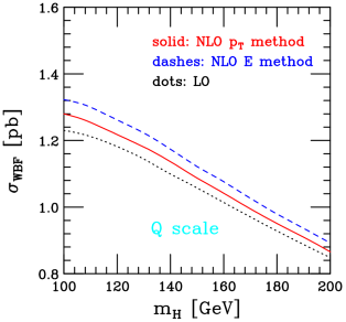
The Higgs boson production cross section, within the above cuts, is shown in Fig. 2 as a function of the Higgs boson mass. QCD corrections increase the LO cross section (dotted line) slightly, by about 3 to 8%, depending on the Higgs boson mass. In addition to our default of identifying the tagging jets as the jets of highest transverse momentum ( method), Fig. 2 also shows the NLO result which is obtained when defining the tagging jets as the two most energetic jets in a given event ( method, dashed line). From a consideration of tagging jet -distributions, the method appears to be somewhat more stable against scale variations, however [10].
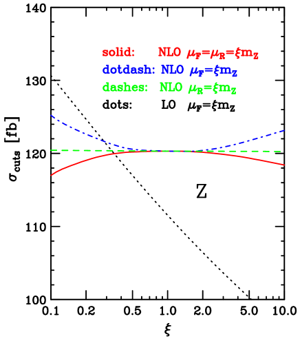
The typical scale dependence of the NLO VBF cross sections is demonstrated in Fig. 3, where the cross section within the cuts of Eqs. (9–12) is shown as a function of the renormalization scale, , holding the factorization scale fixed at (dashed curve), as a function of for (dot-dashed curve) or when varying both. In all cases one finds scale variations at below the 2% level (when allowing variations between and ) which is minute compared to the LO variation (dotted curve). This result holds for Higgs, and production as well as for the scale choice , where denotes the virtuality of the -channel weak bosons in the various VBF processes.
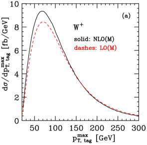
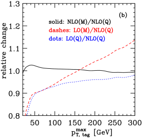
The NLO QCD corrections to observable VBF cross sections are modest, amounting to an increase of less than 10% for in the examples discussed above. Similarly modest QCD corrections are found for most distributions also. One example is shown in Fig. 4, where the tranverse momentum of the hardest tagging jet in events is given. A comparison of the LO (dashed line) and NLO distribution (solid line) in panel (a) exhibits modest shape changes. They are more clearly exposed in Fig. 4(b) where the ratio of distributions
| (13) |
is shown, i.e. we compare to the default scale choice at NLO. Using the mass as the renormalization and factorization scale instead introduces changes below the 2% level at NLO (solid line) which again points to the stability of the NLO predictions. At LO the differential cross section for this scale choice is suppressed by 10% and more at low , and is enhanced by up to 10% at high , i.e. there is a substantial shape change from the LO to the NLO prediction. These changes are somewhat less pronounced when choosing for the LO calculation.
4 Conclusions
The one-loop QCD corrections to Higgs, and production via VBF in hadronic collisions are now available in the form of a flexible NLO parton-level Monte Carlo program. The NLO corrections are modest for cross sections as well as differential distributions at the LHC, rarely exceeding the 10% level. In a variety of distributions one finds shape changes at the 10% level. These changes need to be taken into account in precision studies of VBF processes at the LHC.
References
- [1] ATLAS Collaboration, ATLAS TDR, report CERN/LHCC/99-15 (1999); G. L. Bayatian et al., CMS Technical Proposal, report CERN/LHCC/94-38x (1994).
- [2] D. Rainwater, D. Zeppenfeld and K. Hagiwara, Phys. Rev. D 59, 014037 (1999) [arXiv:hep-ph/9808468]; T. Plehn, D. Rainwater and D. Zeppenfeld, Phys. Rev. D 61, 093005 (2000) [arXiv:hep-ph/9911385]; S. Asai et al., Report No. ATL-PHYS-2003-005.
- [3] D. Rainwater and D. Zeppenfeld, Phys. Rev. D 60, 113004 (1999) [Erratum-ibid. D 61, 099901 (2000)] [arXiv:hep-ph/9906218]; N. Kauer et al., Phys. Lett. B 503, 113 (2001) [arXiv:hep-ph/0012351]; C. M. Buttar, R. S. Harper and K. Jakobs, Report No. ATL-PHYS-2002-033; K. Cranmer et al., Report No. ATL-PHYS-2003-002 and Report No. ATL-PHYS-2003-007; S. Asai et al., Report No. ATL-PHYS-2003-005.
- [4] D. Zeppenfeld, R. Kinnunen, A. Nikitenko and E. Richter-Was, Phys. Rev. D 62, 013009 (2000) [arXiv:hep-ph/0002036]; A. Belyaev and L. Reina, JHEP 0208, 041 (2002) [arXiv:hep-ph/0205270]; M. Dührssen et al., arXiv:hep-ph/0406323.
- [5] H. Chehime and D. Zeppenfeld, Phys. Rev. D 47, 3898 (1993).
- [6] D. Rainwater, R. Szalapski and D. Zeppenfeld, Phys. Rev. D 54, 6680 (1996) [arXiv:hep-ph/9605444].
- [7] V. A. Khoze, M. G. Ryskin, W. J. Stirling and P. H. Williams, Eur. Phys. J. C 26, 429 (2003) [arXiv:hep-ph/0207365].
- [8] U. Baur and D. Zeppenfeld, arXiv:hep-ph/9309227.
- [9] T. Han, G. Valencia and S. Willenbrock, Phys. Rev. Lett. 69, 3274 (1992) [arXiv:hep-ph/9206246].
- [10] T. Figy, C. Oleari and D. Zeppenfeld, Phys. Rev. D 68, 073005 (2003) [arXiv:hep-ph/0306109].
- [11] E. L. Berger and J. Campbell, arXiv:hep-ph/0403194.
- [12] C. Oleari and D. Zeppenfeld, Phys. Rev. D 69 (2004) 093004 [arXiv:hep-ph/0310156].
- [13] S. Catani and M. H. Seymour, Nucl. Phys. B 485, 291 (1997) [Erratum-ibid. B 510, 503 (1997)] [arXiv:hep-ph/9605323].
- [14] S. Catani, Yu. L. Dokshitzer and B. R. Webber, Phys. Lett. B 285 291 (1992); S. Catani, Yu. L. Dokshitzer, M. H. Seymour and B. R. Webber, Nucl. Phys. B406 187 (1993); S. D. Ellis and D. E. Soper, Phys. Rev. D 48 3160 (1993).
- [15] G. C. Blazey et al., arXiv:hep-ex/0005012.
- [16] J. Pumplin et al., JHEP 0207, 012 (2002) [arXiv:hep-ph/0201195].