Nonequilibrium dynamics in scalar hybrid models

Abstract

We study by numerical simulations the transition from the metastable “false vacuum” to the broken symmetry phase in the preheating stage after cosmic inflation in a scalar hybrid model. We take quantum fluctuations and their back reaction into account by applying a one-loop bubble-resummation.[1]

1 Introduction

At present there is a wide class of inflationary models, having in common the aim of explaining various kinds of cosmological puzzles[2]. One of the consecutive questions raised is how inflation has ended. In a scenario called “Hybrid inflation”[3] the inflationary expansion ends by a phase transition from a metastable “false vacuum” to the true, i.e. broken symmetry vacuum. The subsequent phase of (p)reheating[4] after inflation is characterized by a phase of abundant particle production due to spinodal amplification of quantum modes and due to parametric resonance. We will study some aspects of this phase in the following.

2 Effective action and renormalized equations of motion

The Lagrangian for the Hybrid model is given by

$$\mathcal{L} = \frac{1}{2}\partial_{\mu}\Phi\partial^{\mu}\Phi+\frac{1}{2}\partial_{\mu}X\partial^{\mu}X-\frac{1}{2}m^{2}\Phi^{2}-\frac{1}{2}g^{2}\Phi^{2}X^{2}-\frac{\lambda}{4}(X^{2}-v^{2})^{2}\ .$$ (1)

The field $X$ has an effective mass square $m^{2}_{X}(\Phi)=-\lambda v^{2}+g^{2}\Phi^{2}$ and becomes unstable if the absolute value of $\Phi$ is lower than $\Phi_{\mathrm{c}}=\frac{v\sqrt{\lambda}}{g}$ (spinodal region). Both quantum fields $\Phi$ and $X$ are assumed to have classical expectation values, i.e. $\left\langle\Phi\right\rangle=\phi$ (inflaton field) and $\left\langle X\right\rangle=\chi$ (symmetry breaking field).

We will use here the so-called two-particle point-irreducible (2PPI) effective action (EA) formalism. [5, 6] The renormalized equations of motion (EOM) that describe the nonequilibrium dynamics of classical mean fields and their quantum fluctuations, all coupled to each other, are derived from the EA functional

$$\Gamma[\phi,\chi,\Delta_{\{\phi\phi,\phi\chi,\chi\chi\}}] = S[\phi,\chi]+\frac{g^{2}}{2}\int d^{D}x\left(\Delta_{\phi\phi}\Delta_{\chi\chi}+2\Delta_{\phi\chi}^{2}\right)$$

$$+\frac{3\lambda}{4}\int d^{D}x\Delta_{\chi\chi}^{2}+\Gamma^{\mathrm{2PPI}}[\phi,\chi,{\mathcal{M}}^{2}_{\{\phi\phi,\phi\chi,\chi\chi\}}]\ ,$$

$$\Gamma^{\mathrm{2PPI}}[\phi,\chi,{\mathcal{M}}^{2}_{\{\phi\phi,\phi\chi,\chi\chi\}}] = \raisebox{-4.26773pt}{\includegraphics[width=14.22636pt]{figure0a}}+\raisebox{-4.26773pt}{\includegraphics[width=28.45274pt]{figure0b}}+\raisebox{-4.26773pt}{\includegraphics[width=14.22636pt]{figure0c}}+\raisebox{-4.26773pt}{\includegraphics[width=17.07182pt,angle={90}]{figure0d}}+\ldots\ .$$ (3)

The classical EOM follow from $\frac{\delta\Gamma}{\delta\phi}=0$ and $\frac{\delta\Gamma}{\delta\chi}=0$, while the gap equations are derived from $\frac{\delta\Gamma}{{\mathcal{M}}^{2}_{ij}}=0$ with $ij=\phi\phi,\chi\chi$ or $\phi\chi$. The propagator $G$ fulfills a constraint equation

$$(G^{-1})_{ij}(x,x^{\prime})=i\left(\square\delta_{ij}+{\mathcal{M}}^{2}_{ij}(x)\right)\delta^{(D)}(x-x^{\prime})\ .$$ (4)

It is dressed by a resummation of local self-energy insertions. Assuming spatial homogeneous fields, $G_{ij}(t,t^{\prime};\mathbf{p})$ can be decomposed in momentum space into mode functions via $G_{ij}(t,t^{\prime};\mathbf{p})=\sum_{\alpha=1}^{2}\frac{1}{2\omega_{\alpha}}f_{i}^{\alpha}(t;p)f_{j}^{*\,\alpha}(t^{\prime};p)$. The quantities $\omega_{\alpha}$ ($\alpha=1,2$) have to be determined self consistently at the initial time ($t=0$). For practical calculations one has to truncate the infinite series in Eq.(3). Here we will only keep the one-loop term which leads to a summation of bubble diagrams. It is given by $\Gamma^{(1)}[{\mathcal{M}}^{2}_{\phi\phi},{\mathcal{M}}^{2}_{\chi\chi},{\mathcal{M}}^{2}_{\phi\chi}]=\frac{i}{2}\mathrm{Tr}\ln[G^{-1}]$. The tadpole insertions derived from $\Gamma^{(1)}$ denote

$$\Delta_{ij}^{(1)}(t) = -2\frac{\delta\Gamma^{(1)}}{\delta{\mathcal{M}}^{2}_{ij}(t)}=\sum_{\alpha=1}^{2}\int\frac{d^{D-1}p}{(2\pi)^{D-1}}\frac{1}{2\omega_{\alpha}}\mathrm{Re}\left[f_{i}^{\alpha}(t;p)f_{j}^{\alpha\,*}(t;p)\right]\ .$$ (5)

These quantities have quadratic and logarithmic divergencies and have to be renormalized. It turns out[1] that the EA is renormalized by a simple vacuum counter term $\delta E_{\mathrm{vac}}=-\delta\xi[({\mathcal{M}}^{2}_{\phi\phi})^{2}+2({\mathcal{M}}^{2}_{\phi\chi})^{2}+({\mathcal{M}}^{2}_{\chi\chi})^{2}]$, where in dimensional regularization $\delta\xi=-\frac{1}{64\pi^{2}}(\frac{2}{\epsilon}-\gamma+1+\ln 4\pi)$. The vacuum counter term $\delta E_{\mathrm{vac}}$ indeed reflects a resummation of the standard counterterms derived from a counterterm Lagrangian.[5] The renormalized gap equations for the variational parameters ${\mathcal{M}}^{2}_{ij}$ take the form

$${\mathcal{M}}^{2}_{\mathrm{R},\,\phi\phi}(t) = m^{2}+g^{2}\left[\chi^{2}(t)+\Delta_{\chi\chi}(t)\right]-4g^{2}\,\delta\xi{\mathcal{M}}^{2}_{\mathrm{R},\chi\chi}(t)\ ,$$ (6)

$${\mathcal{M}}^{2}_{\mathrm{R},\,\chi\chi}(t) = -\lambda v^{2}+g^{2}\left[\phi^{2}(t)+\Delta_{\phi\phi}(t)\right]+3\lambda\left[\chi^{2}(t)+\Delta_{\chi\chi}(t)\right]$$ (7)

$$-4g^{2}\,\delta\xi{\mathcal{M}}^{2}_{\mathrm{R},\,\phi\phi}(t)-12\lambda\,\delta\xi{\mathcal{M}}^{2}_{\mathrm{R},\,\chi\chi}(t)\ ,$$

$${\mathcal{M}}^{2}_{\mathrm{R},\,\phi\chi}(t) = 2g^{2}\left[\phi(t)\chi(t)+\Delta_{\phi\chi}(t)\right]-8g^{2}\,\delta\xi{\mathcal{M}}^{2}_{\mathrm{R},\,\phi\chi}(t)\ .$$ (8)

The final set of gap equations, with all finite parts from dimensional regularization, is rather lengthy[1] and we don’t write it down here. However, one can see from Eqs. (6)-(8) that the gap equations form a ($3\times 3$) system of linear equations, whose coefficient matrix has to be diagonalized by a time-independent rotation matrix. This fixes the various mass and coupling constant counterterms, obtained from a standard counterterm Lagrangian, in a non-perturbative way.

After all the classical EOM are given by

$$\ddot{\phi}(t)+{\mathcal{M}}^{2}_{\mathrm{R},\,\phi\phi}(t)\phi(t)+{\mathcal{M}}^{2}_{\mathrm{R},\,\phi\chi}(t)\chi(t)-2g^{2}\chi^{2}(t)\phi(t)=0 \!\!,$$ (9)

$$\ddot{\chi}(t)+{\mathcal{M}}^{2}_{\mathrm{R},\,\chi\chi}(t)\chi(t)+{\mathcal{M}}^{2}_{\mathrm{R},\,\phi\chi}(t)\phi(t)-2\lambda\chi^{3}(t)-2g^{2}\phi^{2}(t)\chi(t)=0 \!.$$ (10)

Inserting the decomposition of $G_{ij}(t,t;\mathbf{p})$ into mode functions $f_{i}^{\alpha}(t,p)$ in Eq. (4) the system of EOM for the $f_{i}^{\alpha}(t,p)$ denotes explicitly as

$$\ddot{f}_{\phi}^{\alpha}(t;p)+\mathbf{p}^{2}f_{\phi}^{\alpha}(t;p)+\,{\mathcal{M}}^{2}_{\mathrm{R},\,\phi\phi}(t)f_{\phi}^{\alpha}(t;p)+{\mathcal{M}}^{2}_{\mathrm{R},\,\phi\chi}(t)f_{\chi}^{\alpha}(t;p)=0 \!\!,$$ (11)

$$\ddot{f}_{\chi}^{\alpha}(t;p)+\mathbf{p}^{2}f_{\chi}^{\alpha}(t;p)+\,{\mathcal{M}}^{2}_{\mathrm{R},\,\chi\chi}(t)f_{\chi}^{\alpha}(t;p)+{\mathcal{M}}^{2}_{\mathrm{R},\,\phi\chi}(t)f_{\phi}^{\alpha}(t;p)=0 \!\!.$$ (12)

3 Results

The EOM (9)-(12) are solved numerically. After renormalization the momentum integrals are finite and are carried out using a non-equidistant momentum discretization. In order to simulate the phase transition at the end of inflation we choose the initial amplitudes $\phi(0)>\phi_{\mathrm{c}}$ and $\chi(0)\approx 0$. In particular we take $\phi(0)=1.2$ and $\chi(0)=10^{-7}$. The other parameters are here $m^{2}=0$, $v=1$, $g=2\lambda$, $\lambda=1$.

The time evolution of the classical fields $\phi$ and $\chi$ and of the variational masses is displayed in Fig. 1. One observes three time regimes: (i) the first regime is characterized by a slow-roll of the field $\phi$, where quantum fluctuations are almost negligible; (ii) in the spinodal region the mass ${\mathcal{M}}^{2}_{\chi\chi}$ becomes negative (Fig. 1b). Gaussian fluctuations build up (left column in Fig. 2) and drive ${\mathcal{M}}^{2}_{\chi\chi}$ back to positive values. Along the way the amplitude of $\chi$ growths exponentially; (iii) at later times the momentum spectra display several spikes (see e.g. the right column in Fig. 2) and the symmetry breaking field oscillates around a nonzero value with a relatively constant amplitude. The details in the dynamics depend on the parameters in the model while the characteristic features are very similar.[1]

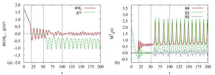
Figure 1: Time evolution of (a) the classical fields $\phi(t)/\phi_{\mathrm{c}}$ (solid line) and $\chi(t)/v$ (dashed line), (b) the effective masses ${\mathcal{M}}^{2}_{ij}(t)$ with $ij={\phi\phi}$ (solid line), $ij={\chi\chi}$ (dashed line) and $ij={\phi\chi}$ (dotted line); the vertical dotted lines indicate the times $19.5$, $51.3$ and $100.2$; parameters: $g^{2}=2\lambda$, $\phi(0)=1.2$, $\chi(0)=1.0\times 10^{-7}$, $m^{2}=0$, $\lambda=1$ and $v^{2}=1$.

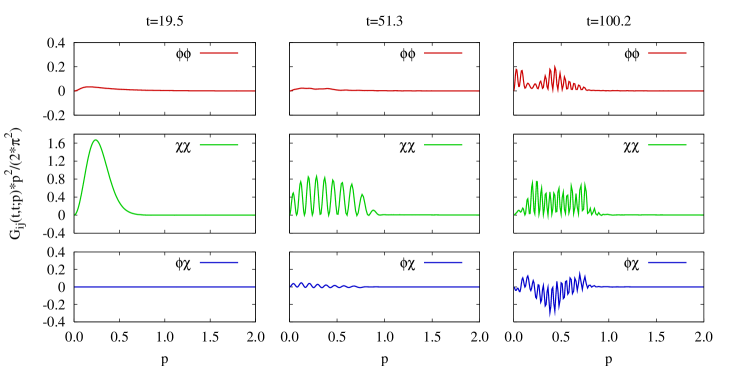
Figure 2: Momentum spectra $G_{ij}(t,t;\mathbf{p})p^{2}/(2\pi^{2})$ for the simulation in Fig. 1 at the times $t=19.5$ (left column), $t=51.3$ (middle column) and $t=100.2$ (right column).

In Fig. 3 we display the time and space evolution of correlations between the fluctuations. One can see that spatial correlations build up in the spinodal region and propagate by twice the speed of light. The correlations decrease once the field $\chi$ starts to oscillate around a non-zero expectation value.

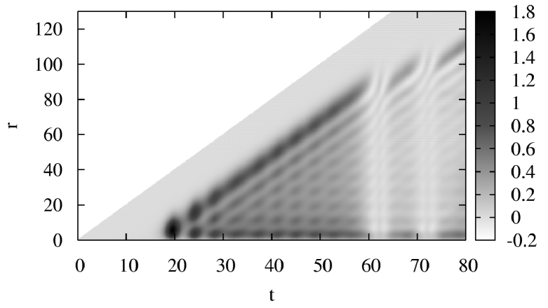
Figure 3:
Correlation function $rC_{\chi\chi}(r,t)=r\int\frac{d^{3}p}{(2\pi)^{3}}e^{i\mathbf{p}\cdot\mathbf{r}}\sum_{\alpha}\frac{1}{2\omega_{\alpha}}\mathrm{Re}[f_{\chi}^{\alpha}f_{\chi}^{*\,\alpha}]$ for the simulation in Fig. 1. The propagation velocity is $r/t=2$ (twice the speed of light).

The decoherence time $t_{\mathrm{dec}}(p)$ for which a given mode becomes classical is defined by $|F_{ij}(t_{\mathrm{dec}},\mathbf{p})|=1$ with $F_{ij}(t,\mathbf{p})=\mathrm{Im}[\sum_{\alpha}\frac{f_{i}^{\alpha*}\dot{f}_{j}^{\alpha}}{2\omega_{\alpha}}]$. The modes right to the curves in Fig. 4 never become classical. The functional dependence is not proportional to $p^{2}$, as found in models with a slow quench where ${\mathcal{M}}^{2}_{\chi\chi}(t)\propto(t_{0}-t)$.

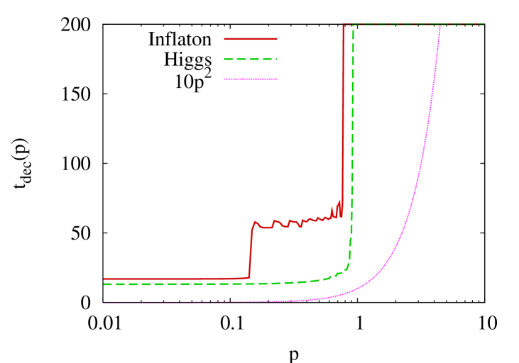
Figure 4: Decoherence time $t_{\mathrm{dec}}(p)$ for which a given mode $p$ becomes “classical” for the simulation in Fig. 1; the solid line represents the inflaton and the dashed line the Higgs modes; the dotted line corresponds to $t_{\mathrm{dec}}\propto p^{2}$.

4 Conclusions

We have analyzed by numerical simulations the transition from the metastable phase to the broken symmetry phase in the Hybrid model. We observed that the back reaction of quantum fluctuations plays an important role and leads, e.g., to a dynamical stabilization in the spinodal region. The approximation used here provides reliable information on the nonequilibrium evolution at earlier times. However, one has to improve further in order to cure, e.g. the lack of dissipation at later times. While there are various improvements, once scattering is taken into account via non-local two-loop diagrams, even in the 2PPI resummation scheme [6], one ultimately wants to achieve a universal late time behavior, i.e. reaching quantum thermalization. The full treatment of the reheating phase remains a desirable goal for future investigations.

AH thanks the GK 841 for partial financial support.

References

- [1] J. Baacke and A. Heinen, Phys. Rev. D 69, 083523 (2004)
- [2] see e.g., D. H. Lyth and A. Riotto, Phys. Rept. 314, 1 (1999).
- [3] A. D. Linde, Phys. Lett. B249, 18 (1990).
- [4] see e.g., G. N. Felder et al., Phys. Rev. Lett. 87, 011601 (2001); E. J. Copeland, D. Lyth, A. Rajantie and M. Trodden, Phys. Rev. D64, 043506 (2001); J. Garcia-Bellido, M. Garcia Perez and A. Gonzalez-Arroyo, Phys. Rev. D67, 103501 (2003); S. Borsanyi, A. Patkos and D. Sexty, Phys. Rev. D68, 063512 (2003).
- [5] H. Verschelde and M. Coppens, Phys. Lett. B287, 133 (1992).
- [6] J. Baacke and A. Heinen, Phys. Rev. D 67, 105020 (2003); ibid. 68, 127702 (2003)