Dynamics of Interacting Scalar Fields in Expanding Space-Time

Abstract

The effective equation of motion is derived for a scalar field interacting with other fields in a Friedman-Robertson-Walker background space-time. The dissipative behavior reflected in this effective evolution equation is studied both in simplified approximations as well as numerically. The relevance of our results to inflation are considered both in terms of the evolution of the inflaton field as well as its fluctuation spectrum. A brief examination also is made of supersymmetric models that yield dissipative effects during inflation.

Version published: Physical Review D71, 023513 (2005)

I Introduction

It is by now well established that inflation models in general have dissipative effects during the inflationary period BGR ; BGR2 ; BR ; BR2 ; BR3 . These effects have two major consequences for inflationary dynamics. First they result in radiation production during inflation, which in turn influences the fluctuations that seed large scale structure. Second they lead to temporally nonlocal terms in the effective evolution equation of the inflaton, which can significantly influence the nature and history of the inflation period. The realization of these dissipative effects in inflation models has resulted in the division of inflation into two dynamical possibilities referred to as cold and warm inflation. Cold inflation is simply the original picture of inflation envisioned in the earliest works oldi ; ni ; ci . In this picture the effects of dissipation are negligible. The fluctuations created during inflation are effectively zero-point ground state fluctuations and the evolution of the inflaton field is governed by a ground state evolution equation. In contrast, in the warm inflation picture wi , inflationary expansion and radiation production occur concurrently. In this picture, the fluctuations created during inflation emerge from some excited statistical state and the evolution of the inflaton has dissipative terms arising from the interaction of the inflaton with other fields.

The dividing point between warm and cold inflation is roughly at $\rho_{r}^{1/4}\approx H$, where $\rho_{r}$ is the radiation energy density present during inflation and $H$ is the Hubble parameter. Thus $\rho_{r}^{1/4}>H$ is the warm inflation regime and $\rho_{r}^{1/4}<H$ is the cold inflation regime. This criteria is independent of thermalization, but if such were to occur, one sees this criteria basically amounts to the warm inflation regime corresponding to when $T>H$. This is easy to understand since the typical inflaton mass during inflation is $m_{\phi}\approx H$ and so when $T>H$, thermal fluctuations of the inflaton field will become important. This criteria for entering the warm inflation regime turns out to require the dissipation of a very tiny fraction of the inflaton vacuum energy during inflation. For example, for inflation with vacuum (i.e. potential) energy at the GUT scale $\sim 10^{15-16}{\rm GeV}$, in order to produce radiation at the scale of the Hubble parameter, which is $\approx 10^{10-11}{\rm GeV}$, it just requires dissipating one part in $10^{20}$ of this vacuum energy density into radiation. Thus energetically not a very significant amount of radiation production is required to move into the warm inflation regime HR . In fact the levels are so small, and their eventual effects on density perturbations and inflaton evolution are so significant, that care must be taken to account for these effects in the analysis of any inflation models.

In recent work BR2 ; BR3 , we have identified a key mechanism which is generic in realistic inflation models and which leads to robust warm inflation. This mechanism involves the scalar inflaton field $\phi$ exciting a heavy bosonic field $\chi$ which then decays to light fermions $\psi_{d}$ BR ,

$$\phi\rightarrow\chi\rightarrow\psi_{d}.$$ (1)

In dynamical terms, this mechanism is expressed in its simplest form by an interaction Lagrangian density for the coupling of the inflaton field to the other fields of the form

$${\cal L}_{I}=-\frac{1}{2}g^{2}\phi^{2}\chi^{2}-g^{\prime}\phi{\bar{\psi}_{\chi}}\psi_{\chi}-h\chi{\bar{\psi}_{d}}\psi_{d},$$ (2)

where $\psi_{d}$ are the light fermions to which $\chi$-particles can decay, with $m_{\chi}>2m_{\psi_{d}}$. Aside from the last term in Eq. (2), these are the typical interactions commonly used in studies of reheating after inflation old ; reheat . However a realistic inflation model often can also have additional interactions outside the inflaton sector, with the inclusion of the light fermions $\psi_{d}$ as depicted above being a viable option. Moreover in minimal supersymmetry (SUSY) extensions of the typical reheating model or multifield inflation models, the interactions of the form as given in Eq. (2) can emerge as an automatic consequence of the supersymmetric structure of the model. Since in the moderate to strong perturbative regime, reheating and multifield inflation models will require SUSY for controlling radiative corrections, Eq. (2) with inclusion of the $\psi_{d}$ field thus is a toy model representative of many realistic situations.

In Ref. BR3 we have presented some results for the above mechanism in a fully expanding space-time dissipative quantum field theory formalism. The primary purpose of this paper is to supply the full details of the formalism used in Ref. BR3 . This paper presents the various approximations used in the derivation, elaborates on the different aspects of dissipative evolution and radiation production and discusses the impact of these results on the density perturbation problem of inflation. Although the formalism presented here has general application, for most of this paper we will focus on the mechanism of Eq. (1). The paper is organized as follows. In Sec. II we compare the inflationary dissipative process associated with Eq. (1) to the reheating process after inflation in the standard cold inflation models. A simple picture of dissipation for both processes is presented. This should help to illustrate the differences between the two processes at work in the two cases. In Sec. III the Lagrangian model studied in this paper is presented. Also this section presents the real time matrix of Green’s functions needed for our calculations and their evolution equations in expanding space-time. In Sec. IV we present approximate solutions for these evolution equations using the WKB ansatz. The derivation of the effective equation of motion for the inflaton field from a response theory approach is done in Sec. V, where we also discuss several simplifying assumptions for the nonlocal terms appearing in the effective equation of motion. These basic equations are then studied numerically in Sec. VI and the validity of the different approximation schemes are explicitly tested for values of parameters of interest to inflation. In Sec. VII we discuss SUSY models that realize the basic interaction structure studied in this paper Eq. (2). In Sec. VIII we study the effects this dissipative process has on density perturbations during inflation. Our concluding remarks are given in Sec. IX. An Appendix is also included where some details are given on the renormalization of the effective equation of motion derived in this paper.

II Interpretation of Dissipation in the linear and nonlinear regimes

It is useful to contrast the dissipation process to be discussed in the following sections to the dissipation process in the (old) reheating studies. For this, consider for instance the typical models for reheating, where an inflaton field $\phi$, with potential $V(\phi)$, is coupled either to spinor fields $\psi$ through the usual Yukawa coupling $h\phi\psi\bar{\psi}$ and/or to other scalar fields $\chi$, with coupling $g^{2}\phi^{2}\chi^{2}$, where in this last case the inflaton potential has symmetry breaking, with minimum at $\phi=\phi_{v}$.

The typical reheating scenario is pictured in the time period just after the inflationary regime, where the inflaton energy density is released in the form of decay products of $\psi$ and/or $\chi$ particles. In the reheating regime the Hubble constant $H$ is smaller than the inflaton mass $m_{\phi}$, which means the inflaton can oscillate about the minimum, $\phi_{v}$, of its potential $V(\phi)$. In addition, to have particle production it requires $m_{\phi}$ to be sufficiently large so $\phi$ can decay, $m_{\phi}>{\rm min}(2m_{\psi},2m_{\chi})$. Typically one takes $m_{\phi}\gg m_{\psi},m_{\chi}$. In this regime the equation of motion is simple to treat for small inflaton amplitude. For example in a quartic inflaton potential with self-coupling $\lambda$, a perturbative treatment is possible under the conditions $\lambda\phi(0)\ll m_{\phi},m_{\chi},m_{\psi}$. In such a regime, the equation of motion for the homogeneous inflaton field $\phi(t)$, including quantum corrections, is given by the general linearized form old

$$\ddot{\phi}(t)+3H\dot{\phi}(t)+\left[m_{\phi}^{2}+\Sigma(k)\right]\phi(t)=0\;,$$ (3)

where $\Sigma(k)$ is the polarization, or self-energy operator for $\phi$, with four-momentum $k=(\omega,0,0,0)$, with $\omega=m_{\phi}$. Due to the condition $m_{\phi}>{\rm min}(2m_{\psi},2m_{\chi})$ the $\phi$ self-energy has a nonzero imaginary part ${\rm Im\Sigma}$. The real part of the self-energy only renormalizes the mass $m_{\phi}$, giving an effective mass to the inflaton, while the imaginary part is associated with the damping of $\phi$ modes due to decay, with the decay rate given by $\Gamma=-{\rm Im}\Sigma(\omega)/(2\omega)$. In the regime ${\rm Im}\Sigma\ll m_{\phi}^{2}$, the solution of (3) ends up being the same as if we just replaced this equation with one having a friction like term proportional to $\Gamma$,

$$\ddot{\phi}(t)+3H\dot{\phi}(t)+m_{\phi}^{2}\phi(t)+\Gamma\dot{\phi}(t)=0\;.$$ (4)

Note that in this derivation, since we are considering the regime $H\ll m_{\phi},m_{\chi},m_{\psi}$, the curvature of the universe is not important in the calculation of the self-energy. As such the decay rate calculation is typically just done in Minkowski space-time. Thus for the two decay processes of interest $\phi\to\chi+\chi$, or $\phi\to\psi+\bar{\psi}$, in the rest frame of the $\phi$-particle the respective decay rates are

$$\Gamma_{\phi\to\chi\chi}=\frac{g^{4}\phi_{v}^{2}}{8\pi m_{\phi}}\;,$$

$$\Gamma_{\phi\to\psi\bar{\psi}}=\frac{h^{2}m_{\phi}}{8\pi}\;,$$ (5)

where we have considered $m_{\phi}\gg m_{\psi},m_{\chi}$. Eq. (4) with Eq, (5) comprise the basic particle production process in the old reheating studies.

Figure 1: The cut in the one-loop self-energy diagram and the amplitude of the decay process associated to it. Full lines stand for the scalar $\phi$ and dotted lines to the spinors $\psi,\bar{\psi}$. Analogous process follow for the decay $\phi\to\chi\chi$.

As is well known weldon , the rates $\Gamma$ also can be expressed in terms of the amplitude square for decay processes. This is illustrated in Fig. 1, where the imaginary term contributing to the rate of decays can be obtained by cutting the diagrams in half. In a dynamical problem, when the $\phi$ modes of given energy $\omega$ and momentum ${\bf k}$ are displaced from equilibrium, these modes get damped and it is the rate $\Gamma$ that describes the approach to equilibrium. This approach to equilibrium is then naturally associated to a dissipative, or irreversible process. This picture is therefore closely related to that of a system (e.g. $\phi$) in interaction with an environment (e.g. the $\chi$ bosons and $\psi$ fermions), in which dissipation (and also noise) results from these interactions. More formally stated in quantum mechanical terms weiss , we describe the state of the system by its reduced density matrix (by integrating out the bath degrees). Due to interactions, the state of the system gets entangled with the state of the bath and therefore some initial pure state of the system will end up turning into a mixture. This is an irreversible process, often called decoherence, that results from the non-unitary system evolution.

We should also point out that although dissipation appears as a generic consequence for a system in interaction with a bath or environment, the simple representation for the dissipation, as in Eq. (4) and the derivation of it, implies a number of simplifying assumptions whose validity need to be checked. For instance, the derivation of Eq. (4) refers just to a very particular regime for the inflaton field, when it is oscillating around the minimum of its potential, with small field amplitudes and in the perturbative regime (or the linear relaxation regime). For this case the effective equation of motion of $\phi$ has the simplified linearized form Eq. (4). This simplified equation would not apply in nonlinear regimes, when large field amplitudes dominate the dynamics, for example in the description for the field modes during preheating, or in any other situation where nonperturbative effects play a relevant role in the description of field dynamics. Even in the linear regimes, Eq. (4) can be shown to be valid only up to a time interval $\Delta t\lesssim 1/\Gamma$ boya , beyond which the decay of $\phi$ is no longer exponential but power law, which itself indicates the break down of the perturbative approximation used to derive Eq. (4). It is clear that in more general cases of large field amplitudes or beyond the perturbative approximation, the expected effective equation of motion for the scalar field $\phi$ must become very different than the simple equation (4). Indeed, in general the effective equation of motion for an arbitrary scalar background field is a nonlocal equation. For example, in the nonlinear regime or for high field amplitudes, the description of the effective dynamics is not a simple local equation of motion (see e.g. Refs. GR ; BGR ; BR ). In addition, as we move away from the regime of validity of linear relaxation dynamics, it may become possible to find other dissipative mechanisms not directly associated to the direct decay process that leads to Eq. (4). In fact, as shown in recent work BR ; BR2 , even in the case where the inflaton can not decay, but fields coupled to it do (actually, $\phi$ does not even need to be the heaviest field), dissipative regimes arise that are not available in the linear or perturbative regime.

An example of interactions leading to a nontrivial inflaton dissipative dynamics is for instance the ones shown in Eq. (2), where now $m_{\chi}>{\rm min}(2m_{\psi_{d}},m_{\phi})$ and $m_{\phi}<{\rm min}(m_{\psi_{\chi}},m_{\chi})$. Here the $\chi$ particles can decay into fermions $\psi_{d}$ that are coupled to it, but there are no kinematically allowed direct decays of $\phi$ into other particles. Nevertheless it is simple to understand from elementary particle physics the origin and nature of dissipation for the inflaton in this case. We look at those processes involving $\phi$ that may have an imaginary term and so in analogy to (3), can be associated to dissipation. This is better interpreted in terms of an effective theory for $\phi$ after integrating over the other fields. We can start doing this by first integrating over the $\psi_{d}$ fermion field. Since this field only couples to $\chi$, its main effect is to dress the $\chi$ scalar propagator, as shown schematically in Fig. 2. Note that the lowest order correction to $\chi$ goes exactly like the previous case analyzed above, in which the $\phi$ field could decay into $\psi$ particles. The leading order one-loop self-energy contribution to $\chi$, $\Sigma_{\chi}(k)$, has a real part that represents a shift in the mass squared of the $\chi$ and an imaginary part that represents the rate of its decay, as is kinematically allowed. This is the same kind of process shown in Fig. 1, by replacing the external lines by $\chi$ and the internal ones by the spinors $\psi_{d}$. Next we can now perform the integration over the (dressed) $\chi$ scalar particles and the $\psi_{\chi}$ spinors coupled to $\phi$. The relevant contributions to our dissipative mechanism are due to the $\chi$ decay (see, however, later in Sec. V a discussion on the role of the $\psi_{\chi}$ spinors). We now have processes contributing to the effective action to $\phi$ like the ones shown in Fig. 3. At leading order, the important contribution to dissipation in the effective equation of motion for $\phi$ arises now from the one-loop vertex diagram shown in Fig. 4. By cutting that diagram in half we are now led to an imaginary contribution that can be seen as a dissipative term appearing in the effective equation of motion of $\phi$. This can be understood from the amplitude shown in Fig. 4, which represents a scattering process of a $\phi$ by a virtual $\chi$ that then decays into the fermion particles. This process can be interpreted in terms of the effective theory for $\phi$, where an evolving background $\phi$-field configuration excites $\phi$-energy modes which then decay into the light fermions $\psi_{d}$, with that decay mediated by (virtual) $\chi$ particles. The resulting dissipative term appearing in the effective equation of motion for $\phi$ can be seen from the square amplitude shown in Fig. 4 to be of order ${\cal O}(\phi^{2}g^{4}\Gamma_{\chi\to\psi_{d}\bar{\psi}_{d}})$. This result is in fact corroborated by the explicit derivation of the dissipation term in Sec. V. We can also note that this result is nonlinear in the $\phi$ field amplitude, since it originates from a scattering process (involving two $\phi$ particles and two virtual $\chi$ particles) and it is nonperturbative in nature, since it involves the dressed $\chi$ propagators based on a resummation, which means that physically the $\phi$ field is not interacting with vacuum like $\chi$ excitations but rather with the collective $\chi$ excitations.

Figure 2: The lowest order terms of the effective propagator for the scalar $\chi$ after integrating over the fermion fields coupled to it. The black ellipse stand for the spinors quantum corrections and the dashed lines to the $\chi$ propagator.

It should be noted that the dissipative processes as represented in Fig. 4 are of higher order than the ones shown in Fig. 1. However, due to the nontrivial nature of the latter, they may become important in those regimes characterized by high $\phi$ amplitudes (and then outside the region of validity of linear relaxation theory), and couplings ($g$ and $h$ in Eq. (2)) that are not perturbatively small. It is exactly in this region of parameters, that we will find the relevance to inflationary dynamics of the nonlinear dissipative mechanism discussed here and derived in this paper.

Figure 3: Some of the lowest order diagrams contributing to the action of $\phi$ after integrating over the scalar $\chi$ and spinors $\psi_{d},\bar{\psi}_{d}$.

Figure 4: The cut in the lowest order nontrivial diagram appearing in the effective action of $\phi$ that has an imaginary part and the main amplitude associated to it.

III A working model of a scalar field in interaction with multiple other fields

Consider the following model initially presented in BR2 , which consists of a scalar field $\Phi$ interacting with a set of scalar fields $\chi_{j}$, $j=1,\ldots,N_{\chi}$ and these scalar fields in turn interact with fermion fields $\psi_{k}$, $k=1,\ldots,N_{\psi}$. Here we work in the FRW background metric $ds^{2}=dt^{2}-a(t)^{2}d{\bf x}^{2}$. The Lagrangian density for the matter fields coupled to the gravitational field tensor $g_{\mu\nu}$ is given by

$${\cal L}[\Phi,\chi_{j},\bar{\psi}_{k},\psi_{k},g_{\mu\nu}] = \sqrt{-g}\left\{\frac{1}{2}g^{\mu\nu}\partial_{\mu}\Phi\partial_{\nu}\Phi-\frac{m_{\phi}^{2}}{2}\Phi^{2}-\frac{\lambda}{4!}\Phi^{4}-\frac{\xi}{2}R\Phi^{2}\right.$$ (6)

$$+ \left.\sum_{j=1}^{N_{\chi}}\left[g^{\mu\nu}\frac{1}{2}\partial_{\mu}\chi_{j}\partial_{\nu}\chi_{j}-\frac{m_{\chi_{j}}^{2}}{2}\chi_{j}^{2}-\frac{f_{j}}{4!}\chi_{j}^{4}-\frac{g_{j}^{2}}{2}\Phi^{2}\chi_{j}^{2}-\frac{\xi}{2}R\chi_{j}^{2}\right]\right.$$

$$+ \left.\sum_{k=1}^{N_{\psi}}\left[i\psi_{k}\gamma^{\mu}\left(\partial_{\mu}+\omega_{\mu}\right)\psi_{k}-\bar{\psi}_{k}\left(m_{\psi_{k}}+\sum_{j=1}^{N_{\chi}}h_{kj,\chi}\chi_{j}\right)\psi_{k}\right]\right\}\>,$$

where $R$ is the curvature scalar,

$$R=6\left(\frac{\ddot{a}}{a}+\frac{\dot{a}^{2}}{a^{2}}\right)\;,$$ (7)

$\xi$ is the dimensionless parameter describing the coupling of the matter fields to the gravitational background and all coupling constants are positive: $\lambda$, $f_{j},g_{j}^{2},h_{kj,\chi}$ $>0$. In the last term involving the fermion fields, the $\gamma^{\mu}$ matrices are related to the vierbein $e_{\mu}^{a}$ (where $g_{\mu\nu}=e_{\mu}^{a}e_{\nu}^{b}\eta_{ab}$, with $\eta_{ab}$ the usual Minkowski metric tensor) by mallik $\gamma^{\mu}(x)=\gamma^{a}e_{a}^{\mu}(x)$, where $\gamma^{a}$ are the usual Dirac matrices and $\omega_{\mu}=-(i/4)\sigma^{ab}e_{a}^{\nu}\nabla_{\mu}e_{b\nu}$, with $\sigma^{ab}=i[\gamma^{a},\gamma^{b}]/2$.

We are interested in obtaining the effective equation of motion (EOM) for a scalar field configuration $\varphi=\langle\Phi\rangle$ after integrating out the $\Phi$ fluctuations, the scalars $\chi_{j}$ and spinors $\psi_{k},\bar{\psi}_{k}$. This is a typical ”system-environment” decomposition of the problem in which $\varphi$ is regarded as the system field and everything else is the environment, which in particular means the $\Phi$ fluctuation modes, the scalars $\chi_{j}$ and the spinors $\psi_{k},\bar{\psi}_{k}$ are regarded as the environment bath. In a Minkowski background, at $T=0$, the EOM for $\varphi$ has been derived in BR using the Schwinger closed time path formalism. Here we follow a completely analogous approach and derive the EOM in a FRW background. The field equation for $\Phi$ can be readily obtained from Eq. (6) and it is given by

$$\ddot{\Phi}+3\frac{\dot{a}}{a}\dot{\Phi}-\frac{\nabla^{2}}{a^{2}}\Phi+m_{\phi}^{2}\Phi+\frac{\lambda}{6}\Phi^{3}+\xi R\Phi+\sum_{j=1}^{N_{\chi}}g_{j}^{2}\Phi(x)\chi_{j}^{2}(x)=0\;.$$ (8)

In order to obtain the effective EOM for $\varphi$, we use the tadpole method. In this method we split $\Phi$ in Eq. (8), as usual, into the (homogeneous) classical expectation value $\varphi(t)=\langle\Phi\rangle$ and a quantum fluctuation $\phi(x)$, $\Phi(x)=\varphi(t)+\phi(x)$. This way, the field equation for $\Phi$, after taking the average (with $\langle\phi(x)\rangle=0$), becomes

$$\ddot{\varphi}(t)+3\frac{\dot{a}(t)}{a(t)}\dot{\varphi}(t)+m_{\phi}^{2}\varphi(t)+\frac{\lambda}{6}\varphi^{3}(t)+\xi R(t)\varphi(t)+\frac{\lambda}{2}\varphi(t)\langle\phi^{2}\rangle+\frac{\lambda}{6}\langle\phi^{3}\rangle$$ (9)

$$+ \sum_{j=1}^{N_{\chi}}g_{j}^{2}\left[\varphi(t)\langle\chi_{j}^{2}\rangle+\langle\phi\chi_{j}^{2}\rangle\right]=0\;,$$

where $\langle\phi^{2}\rangle$, $\langle\phi^{3}\rangle$, $\langle\chi_{j}^{2}\rangle$ and $\langle\phi\chi_{j}^{2}\rangle$ can be expressed BR in terms of the coincidence limit of the (causal) two-point Green’s functions $G^{++}_{\phi}(x,x^{\prime})$ and $G^{++}_{\chi_{j}}(x,x^{\prime})$, for the $\Phi$ and $\chi_{j}$ fields respectively. These Green’s functions are appropriately defined in the context of the Schwinger closed time path (CTP) formalism CTP . They are obtained from the $(1,1)$-component of the real time matrix of effective propagators, which satisfy the appropriate Schwinger-Dyson equations (see, e.g., ian ; BGR for further details). These equations satisfied by the effective (or dressed) propagators emerge from the successive integrations over the bath fields in (6). The integration over the spinors $\psi_{k},\bar{\psi}_{k}$ leads to dressed propagators for the $\chi_{j}$ fields (see e.g. Fig. 2), which are then given by (in the FRW background)

$$\left[\frac{\partial^{2}}{\partial t^{2}}+3\frac{\dot{a}}{a}\frac{\partial}{\partial t}-\frac{\nabla^{2}}{a^{2}}+m_{\chi_{j}}^{2}+g_{j}^{2}\varphi(t)^{2}+\xi R(t)\right]G_{\chi_{j}}(x,x^{\prime})+\int d^{4}z\Sigma_{\chi_{j}}(x,z)G_{\chi_{j}}(z,x^{\prime})=i\frac{\delta(x,x^{\prime})}{a^{3/2}(t)a^{3/2}(t^{\prime})}\;,$$ (10)

where $\Sigma_{\chi_{j}}(x,y)$ is the self-energy for $\chi_{j}$ due to the coupling to the spinors $\psi_{k},\bar{\psi}_{k}$. Next, by integrating over the $\chi_{j}$ and $\phi$ fluctuations we are left with an effective propagator for the $\Phi$ fields that is also formally defined by

$$\left[\frac{\partial^{2}}{\partial t^{2}}+3\frac{\dot{a}}{a}\frac{\partial}{\partial t}-\frac{\nabla^{2}}{a^{2}}+m_{\phi}^{2}+\frac{\lambda}{2}\varphi(t)^{2}+\xi R(t)\right]G_{\phi}(x,x^{\prime})+\int d^{4}z\Sigma_{\phi}(x,z)G_{\phi}(z,x^{\prime})=i\frac{\delta(x,x^{\prime})}{a^{3/2}(t)a^{3/2}(t^{\prime})}\;,$$ (11)

where $\Sigma_{\phi}(x,y)$ denotes now the self-energy for $\Phi$ after integrating over the remaining bath fields.

In the CTP formalism of quantum field theory, Eqs. (10) and (11) are matrix equations for the propagators and self-energies, where, for instance, by expressing $G_{\phi}(x,x^{\prime})$ in terms of its momentum-space Fourier transform (and analogously for $G_{\chi_{j}}$), it can be expressed in the form

$$G_{\phi}(x,x^{\prime})=i\int\frac{d^{3}q}{(2\pi)^{3}}e^{i{\bf q}.({\bf x}-{\bf x}^{\prime})}\left(\begin{array}[]{ll}G^{++}_{\phi}({\bf q},t,t^{\prime})&\>\>G^{+-}_{\phi}({\bf q},t,t^{\prime})\\ G^{-+}_{\phi}({\bf q},t,t^{\prime})&\>\>G^{--}_{\phi}({\bf q},t,t^{\prime})\end{array}\right)\>,$$ (12)

where

$$G^{++}_{\phi}({\bf q},t,t^{\prime})=G^{>}_{\phi}({\bf q},t,t^{\prime})\theta(t-t^{\prime})+G^{<}_{\phi}({\bf q},t,t^{\prime})\theta(t^{\prime}-t),$$

$$G^{--}_{\phi}({\bf q},t,t^{\prime})=G^{>}_{\phi}({\bf q},t,t^{\prime})\theta(t^{\prime}-t)+G^{<}_{\phi}({\bf q},t,t^{\prime})\theta(t-t^{\prime}),$$

$$G^{+-}_{\phi}({\bf q},t,t^{\prime})=G^{<}_{\phi}({\bf q},t,t^{\prime}),$$

$$G^{-+}_{\phi}({\bf q},t,t^{\prime})=G^{>}_{\phi}({\bf q},t,t^{\prime})\;,$$ (13)

with each matrix element defined in terms of two-point correlations of the fields that are on each branch of the CTP contour CTP . In writing (12) we are assuming that $G(x,x^{\prime})$ only depends on the difference ${\bf x}-{\bf x}^{\prime}$, which follows for homogeneous field configurations, as is our interest here. The elements of the propagator matrix, Eq. (13), for both the scalars bosons $\phi$ and $\chi_{j}$, are found to satisfy the conditions

$$G^{>}(x,x^{\prime})=G^{<}(x^{\prime},x)\;,$$

$$\left[iG^{>(<)}(x,x^{\prime})\right]^{\dagger}=iG^{<(>)}(x,x^{\prime})\;,$$

$$\left[G^{>(<)}({\bf q},t,t^{\prime})\right]^{\dagger}=G^{>(<)}({\bf q},t^{\prime},t)\;,$$

$$\frac{d}{dt}\left[G^{>}({\bf q},t,t^{\prime})-G^{>}({\bf q},t^{\prime},t)\right]\Bigr{|}_{t=t^{\prime}}=i\delta(t-t^{\prime})\;,$$ (14)

where the third condition in (14) is just a result of the first two conditions. The definitions of the retarded and advanced propagators are also given in terms of the matrix elements of the two-point function in the CTP formalism:

$$G^{\rm ret}(x,x^{\prime})=\theta(t-t^{\prime})\left[G^{>}(x,x^{\prime})-G^{<}(x,x^{\prime})\right]=G^{++}(x,x^{\prime})-G^{+-}(x,x^{\prime})\;,$$ (15)

$$G^{\rm adv}(x,x^{\prime})=\theta(t^{\prime}-t)\left[G^{<}(x,x^{\prime})-G^{>}(x,x^{\prime})\right]=G^{++}(x,x^{\prime})-G^{-+}(x,x^{\prime})\;.$$ (16)

In particular, we have the known result that $G^{\rm ret}(x,x^{\prime})=G^{\rm adv}(x^{\prime},x)$.

The self-energy matrix elements are also expressed in a similar way to the propagators in the CTP formalism as

$$\Sigma_{\phi}^{++}(x,x^{\prime})=\Sigma_{\phi}^{>}(x,x^{\prime})\theta(t-t^{\prime})+\Sigma_{\phi}^{<}(x,x^{\prime})\theta(t^{\prime}-t),$$

$$\Sigma_{\phi}^{--}(x,x^{\prime})=\Sigma_{\phi}^{>}(x,x^{\prime})\theta(t^{\prime}-t)+\Sigma_{\phi}^{<}(x,x^{\prime})\theta(t-t^{\prime}),$$

$$\Sigma_{\phi}^{+-}(x,x^{\prime})=-\Sigma^{<}_{\phi}(x,x^{\prime}),$$

$$\Sigma^{-+}_{\phi}(x,x^{\prime})=-\Sigma^{>}_{\phi}(x,x^{\prime})\;,$$ (17)

with analogous expressions for the $\chi_{j}$ self-energy elements. From (17) the following property follows,

$$\Sigma^{++}(x,x^{\prime})+\Sigma^{+-}(x,x^{\prime})+\Sigma^{-+}(x,x^{\prime})+\Sigma^{--}(x,x^{\prime})=0\;.$$ (18)

In addition the elements in (17) are found in general to satisfy conditions similar to those in (14), which are valid for both the scalar bosons $\phi$ and $\chi_{j}$,

$$\Sigma^{>}(x,x^{\prime})=\Sigma^{<}(x^{\prime},x)\;,$$

$$\left[i\Sigma^{>(<)}(x,x^{\prime})\right]^{\dagger}=i\Sigma^{<(>)}(x,x^{\prime})\;.$$ (19)

In terms of Eq. (17) and the equations for the fluctuation field modes derived from Eq. (6), we can write general expressions for the solutions for the $G^{>(<)}$ propagator functions. For instance, consider the fluctuations equation for the $\chi_{j}$ fields that can be obtained after integrating over the fermion $\psi_{k},\bar{\psi}_{k}$. This equation is obtained from the quadratic action in the $\chi_{j}$ scalar fields, $S_{2}[\chi_{j}]$ obtained from Eq. (6). In the CTP formalism it is obtained by identifying fields in each branch of the Schwinger’s closed time path contour, with fields in the forward and backward segments of the CTP time contour identified as $\chi_{j}^{+}$ and $\chi_{j}^{-}$, respectively (see e.g. GR ). In term of these fields, we can express the quadratic action for the $\chi_{j}$ fields, after integration over the fermions as

$$S_{2}[\chi_{j}^{+},\chi_{j}^{-}] = \frac{1}{2}\int d^{4}xa^{3}(t)\left\{\left[\left(\frac{\partial\chi_{j}^{+}}{\partial t}\right)^{2}-\chi_{j}^{+}\left(-\frac{\nabla^{2}}{a^{2}(t)}+M_{\chi_{j}}^{2}\right)\chi_{j}^{+}\right]-\left[\left(\frac{\partial\chi_{j}^{-}}{\partial t}\right)^{2}-\chi_{j}^{-}\left(-\frac{\nabla^{2}}{a^{2}(t)}+M_{\chi_{j}}^{2}\right)\chi_{j}^{-}\right]\right\}$$ (20)

$$- \int d^{4}xa^{3}(t)\int d^{4}x^{\prime}a^{3}(t^{\prime})\;\frac{1}{2}\left[\chi_{j}^{+}(x)\Sigma_{\chi_{j}}^{++}(x,x^{\prime})\chi_{j}^{+}(x^{\prime})+\chi_{j}^{+}(x)\Sigma_{\chi_{j}}^{+-}(x,x^{\prime})\chi_{j}^{-}(x^{\prime})\right.$$

$$\left.~{}~{}~{}~{}~{}~{}~{}~{}~{}~{}~{}~{}~{}~{}~{}~{}~{}~{}~{}~{}~{}~{}~{}~{}~{}~{}~{}~{}~{}~{}~{}~{}+\chi_{j}^{-}(x)\Sigma_{\chi_{j}}^{-+}(x,x^{\prime})\chi_{j}^{+}(x^{\prime})+\chi_{j}^{-}(x)\Sigma_{\chi_{j}}^{--}(x,x^{\prime})\chi_{j}^{-}(x^{\prime})\right]\;,$$

where $M_{\chi_{j}}^{2}=m_{\chi_{j}}^{2}+g_{j}^{2}\varphi^{2}(t)+\xi R(t)$, $\varphi(t)$ is the background $\Phi$ field, and $\Sigma_{\chi_{j}}(x,x^{\prime})$ denotes the fermion loop contributions, which dress the $\chi_{j}$ fields. It is now useful to use in Eq. (20) the redefined fields given by GR

$$\chi_{j}^{c}=\frac{1}{2}\left(\chi_{j}^{+}+\chi_{j}^{-}\right)\;,$$

$$\chi_{j}^{\Delta}=\chi_{j}^{+}-\chi_{j}^{-}\;,$$ (21)

along with the identity (18), which lead to the result

$$S_{2}[\chi_{j}^{c},\chi_{j}^{\Delta}] = \int d^{4}xa^{3}(t)\left[\chi_{j}^{\Delta}\left(-\frac{\partial^{2}}{\partial t^{2}}-3\frac{\dot{a}}{a}\frac{\partial}{\partial t}+\frac{\nabla^{2}}{a^{2}}-M_{\chi_{j}}^{2}\right)\chi_{j}^{c}\right]$$ (22)

$$- \int d^{4}xa^{3}(t)\int d^{4}x^{\prime}a^{3}(t^{\prime})\left\{\chi_{j}^{\Delta}(x)\left[\Sigma_{\chi_{j}}^{++}(x,x^{\prime})+\Sigma_{\chi_{j}}^{+-}(x,x^{\prime})-\Sigma_{\chi_{j}}^{-+}(x,x^{\prime})-\Sigma_{\chi_{j}}^{--}(x,x^{\prime})\right]\chi_{j}^{c}(x^{\prime})\right.$$

$$\left.~{}~{}~{}~{}~{}~{}~{}~{}~{}~{}~{}~{}~{}~{}~{}~{}~{}~{}~{}~{}~{}~{}~{}~{}~{}~{}~{}-\chi_{j}^{\Delta}(x)\left[\Sigma_{\chi_{j}}^{++}(x,x^{\prime})-\Sigma_{\chi_{j}}^{+-}(x,x^{\prime})-\Sigma_{\chi_{j}}^{-+}(x,x^{\prime})+\Sigma_{\chi_{j}}^{--}(x,x^{\prime})\right]\chi_{j}^{\Delta}(x^{\prime})\right\}\;.$$

Using Eqs. (17) and (18), the argument involving the self-energies in the second term in Eq. (22) becomes

$$\Sigma_{\chi_{j}}^{++}(x,x^{\prime})+\Sigma_{\chi_{j}}^{+-}(x,x^{\prime})-\Sigma_{\chi_{j}}^{-+}(x,x^{\prime})-\Sigma_{\chi_{j}}^{--}(x,x^{\prime})$$

$$=2\left[\Sigma_{\chi_{j}}^{++}(x,x^{\prime})+\Sigma_{\chi_{j}}^{+-}(x,x^{\prime})\right]=2\theta(t_{1}-t_{2})\left[\Sigma_{\chi_{j}}^{>}(x,x^{\prime})-\Sigma_{\chi_{j}}^{<}(x,x^{\prime})\right]$$

$$=\Pi_{\chi_{j}}(x,x^{\prime})=\Pi_{1,\chi_{j}}(x,x^{\prime})+\Pi_{2,\chi_{j}}(x,x^{\prime})\;,$$ (23)

where

$$\Pi_{1,\chi_{j}}(x,x^{\prime})=\left[2\theta(t_{1}-t_{2})-1\right]\left[\Sigma_{\chi_{j}}^{>}(x,x^{\prime})-\Sigma_{\chi_{j}}^{<}(x,x^{\prime})\right]\;,$$

$$\Pi_{2,\chi_{j}}(x,x^{\prime})=\Sigma_{\chi_{j}}^{>}(x,x^{\prime})-\Sigma_{\chi_{j}}^{<}(x,x^{\prime})\;,$$ (24)

which, from (19) have the properties $\Pi_{1,\chi_{j}}(x,x^{\prime})=\Pi_{1,\chi_{j}}(x^{\prime},x)$ and $\Pi_{2,\chi_{j}}(x,x^{\prime})=-\Pi_{2,\chi_{j}}(x^{\prime},x)$. Similarly, the self-energy contributions in the third term in Eq. (22) can be written as

$$\Sigma_{\chi_{j}}^{++}(x,x^{\prime})-\Sigma_{\chi_{j}}^{+-}(x,x^{\prime})-\Sigma_{\chi_{j}}^{-+}(x,x^{\prime})+\Sigma_{\chi_{j}}^{--}(x,x^{\prime})$$

$$=2\left[\Sigma_{\chi_{j}}^{>}(x,x^{\prime})+\Sigma_{\chi_{j}}^{<}(x,x^{\prime})\right]=2i{\rm Im}\left[\Sigma_{\chi_{j}}^{>}(x,x^{\prime})+\Sigma_{\chi_{j}}^{<}(x,x^{\prime})\right]\;,$$ (25)

where the last equality in (25) follows from (19), from which we see that $\Sigma_{\chi_{j}}^{>}(x,x^{\prime})+\Sigma_{\chi_{j}}^{<}(x,x^{\prime})$ must be purely imaginary.

By substituting Eqs. (23) and (25) in (22), due to the result (25), we are led to an imaginary contribution to the effective action for the $\chi_{j}$ fields. This imaginary term can be appropriately interpreted as coming from a functional integral over a stochastic field, which then turns the evolution equation for $\chi_{j}$ into a stochastic form due to the presence of a noise term GR . Thus the complete evolution equation for the modes and background fields includes noise terms. Though their study is particularly difficult, previous estimates of their effects on the background dynamics during inflation and reheating hu shows that changes in the dynamics and energy densities are marginal for chaotic inflation kind of models and within parameters values for coupling constants ($\lambda,g_{j},h_{k}$) corresponding to the cases of interest in this paper. Due to this we can neglect the stochastic noise terms appearing in (22). On the other hand these noise terms are important in obtaining the first principles evolution equation for the fluctuating modes of the inflaton, such as for studying density fluctuations during inflation; however in this paper we will not go that far. Thus by defining the evolution equation for $\chi_{j}$ modes from GR ,

$$\frac{\delta S_{2}[\chi_{j}^{c},\chi_{j}^{\Delta}]}{\chi_{j}^{\Delta}}\Bigr{|}_{\chi_{j}^{\Delta}=0}=0\;,$$ (26)

we are led to the following equation for the $\chi_{j}$ modes $f_{\chi_{j}}({\bf q},t)$ in momentum space

$$\left[\frac{d^{2}}{dt^{2}}+3\frac{\dot{a}}{a}\frac{\partial}{\partial t}+\frac{\bf{q}^{2}}{a^{2}}+M_{\chi_{j}}^{2}(t)\right]f_{\chi_{j}}({\bf q},t)+\int dt^{\prime}a^{3}(t^{\prime})\Pi_{\chi_{j}}({\bf q};t,t^{\prime})f_{\chi_{j}}({\bf q},t^{\prime})=0\;,$$ (27)

where $\Pi_{\chi_{j}}({\bf q};t,t^{\prime})$ is the spatial Fourier transform of the $\chi_{j}$ field self-energy term given by Eq. (23). An analogous expression for the fluctuation $\phi$ modes also follows, like Eq. (27), with $M_{\phi}^{2}(t)=m_{\phi}^{2}+\frac{\lambda}{2}\varphi(t)^{2}+\xi R(t)$ and self-energies terms coming from the dressing due to $\chi_{j}$ and $\phi$ loops. The initial conditions for these field mode differential equations will be explicitly stated below for the case of conformal time. Though this is not of special concern in this work, this is a convenient way to circumvent known subtle issues of renormalization dependence on the initial conditions in gravitational backgrounds when formulated in comoving time davis .

In terms of the general solutions of (27), $f_{1,2}({\bf q},t)$ and their complex conjugate solutions, obtained equivalently from e.g. the complex conjugate of Eq. (27) (note that when the bath self-energy term entering in (27) has an imaginary part, the equation becomes non-Hermitian), we then can write general expressions for the CTP propagator terms, for both the scalars $\phi$ and $\chi_{j}$, in agreement with the continuity conditions expressed in Eq. (14), in the general form semeno ; mallik2

$$G^{>}({\bf q},t,t^{\prime})=f_{1}({\bf q},t)f_{2}({\bf q},t^{\prime})\theta(t-t^{\prime})+f^{*}_{1}({\bf q},t^{\prime})f^{*}_{2}({\bf q},t)\theta(t^{\prime}-t)\;,$$

$$G^{<}({\bf q},t,t^{\prime})=f_{1}^{*}({\bf q},t)f_{2}^{*}({\bf q},t^{\prime})\theta(t-t^{\prime})+f_{1}({\bf q},t^{\prime})f_{2}({\bf q},t)\theta(t^{\prime}-t)\;.$$ (28)

The solutions $f_{1,2}({\bf q},t)$ and the appropriated initial conditions needed to determine them are discussed below.

IV Solving for the mode functions and real time interacting propagators

Typically, equations for the mode functions for an interacting model, of the general form as given by Eq. (27), can be very difficult to solve analytically, in particular for an expanding background. There are, however, a few particular cases, like for de Sitter expansion $H\sim$ constant, so $a(t)=\exp(Ht)$, and power law expansion $a(t)\sim t^{n}$, where solutions for the mode equation for free fluctuations are known in exact analytical form (see e.g. Ref. davis ). For instance the mode equation for free fluctuations in de Sitter is (where in this case the scalar of curvature becomes $R=12H^{2}$)

$$\left[\frac{d^{2}}{dt^{2}}+3H\frac{d}{dt}+{\bf q}^{2}e^{-2Ht}+m^{2}+12\xi H^{2}\right]f_{\rm de\,Sitter}({\bf q},t)=0\;,$$ (29)

which has known solutions given in terms of Bessel functions of first and second kind,

$$f_{1,2}({\bf q},t)\sim J_{\nu}\left(qe^{-Ht}/H\right),\;\;Y_{\nu}\left(qe^{-Ht}/H\right)\;,$$ (30)

with $\nu=-i\sqrt{m^{2}/H^{2}+12\xi-9/4}$. The other case where we can find an exact solution for the modes corresponds to power law expansion, where, by considering $a(t)=(t/t_{0})^{n}$ and massless (free) fields with minimal coupling ($\xi=0$), the solutions are given by habib

$$f_{1,2}({\bf q},t)\sim t^{1/2}H_{\mu}^{(1)}\left(\frac{qt_{0}^{n}t^{1-n}}{n-1}\right),\;\;t^{1/2}H_{\mu}^{(2)}\left(\frac{qt_{0}^{n}t^{1-n}}{n-1}\right)\;,$$ (31)

with $\mu=(1-3n)/[2(1-n)]$ and $H_{\mu}^{(1,2)}(x)=J_{\nu}(x)\pm iY_{\nu}(x)$ are the Hankel functions.

Alternatively, for deriving an approximate solution for the mode functions in the interacting case, we can apply a WKB approximation for equations of the general form Eq. (27) and then check the validity of the approximation for the parameter and dynamical regime of interest to us. As will be seen below, under the dynamical conditions we are interested in studying in this paper, this approximation will suit our purposes. Let us briefly recall the WKB approximation and its general validity regime, when applied to obtaining approximate solutions for field mode equations. An approximated WKB solution for a mode equation like

$$\left[\frac{d^{2}}{dt^{2}}+\omega^{2}({\bf q},t)\right]f({\bf q},t)=0\;,$$ (32)

is of the form $f_{WKB}({\bf q},t)=1/\left[\omega({\bf q},t)\right]^{1/2}\exp\left[\pm i\int^{t}dt^{\prime\prime}\omega({\bf q},t^{\prime\prime})\right]$, which holds under the general adiabatic condition $\dot{\omega}({\bf q},t)\ll\omega^{2}({\bf q},t)$. We must point out that there is no problems in extending this approximation to an expanding background and in fact it is a common approximation taken for instance in the analysis of perturbation modes in the adiabatic regime wkbad . In that case, however, massless modes are considered and so the approximation holds only for large enough physical momenta $q/a\gg H$, corresponding to wavelengths deep inside the horizon. Here, instead, we work in the large mass scale regime, e.g. $m_{\chi}\gg H$. In this regime the WKB approximation is also valid. This can easily be checked by comparing the WKB solution $f_{WKB}$ with the one obtained from the exact solution for the modes equations, e.g., given by (30), $f_{exact}(q,t)$, for free fields in de Sitter spacetime. For example, it is useful to examine the ratio $|f_{WKB}/f_{exact}|$. For both solutions the same initial/boundary conditions are taken (in conformity to the Bunch-Davies vacuum davis ) at $t_{0}$ (and lets say $t_{0}=0$), so both results match at the initial time. They also match in the asymptotic $q\to\infty$ or $H\to 0$ limits, as they should, so as to correctly reproduce the Minkowski results. But they are also found to match very well for masses $m\gg H$, independent of the value of the physical momenta (in particular even for $q/a\ll H\ll m$). For example, it can easily be checked that for (in units of $H$) $\xi=0$, $q/a=0.01H$ and for $m=10H$, the overall numerical difference between the exact and approximated WKB forms for the modes is at most not more than one percent for an evolution in the first 10 e-folds and this discrepancy gets smaller for longer evolutions. For the typical parameters we consider in this work (in Sec. VI) and relevant for the dissipation mechanism discussed in Sec. II, we have for example $m_{\chi}\stackrel{{\scriptstyle>}}{{\sim}}10^{6}H$, and so the WKB approximation is expected to be excellent, which is indeed confirmed by the numerical results to be shown later in this paper. In addition, note also that large mass scales, $m\gg H$, imply that curvature effects in the field quantum corrections to be considered for the background inflaton field are subleading, with the dominant terms being the Minkowski like corrections.

Proceeding with our derivations, consider then a differential equation in the form of Eq. (27). Instead of working in cosmic time, it is more convenient to work in conformal time $\tau$, defined by $d\tau=dt/a(t)$, in which case the metric becomes conformally flat,

$$ds^{2}=a(\tau)^{2}\left(d\tau^{2}-d{\bf x}^{2}\right)\;,$$ (33)

By also defining a rescaled mode field in conformal time by

$$\frac{1}{a(\tau)}\bar{f}({\bf q},\tau)=f({\bf q},t)\;,$$ (34)

we can then re-express Eq. (27) in the form (generically valid for either $\phi$ or $\chi_{j}$ scalar fluctuations)

$$\frac{d^{2}}{d\tau^{2}}\bar{f}({\bf q},\tau)+\bar{\omega}({\bf q},\tau)^{2}\bar{f}({\bf q},\tau)+\int d\tau^{\prime}\bar{\Pi}({\bf q},\tau,\tau^{\prime})\bar{f}({\bf q},\tau^{\prime})=0\;,$$ (35)

where we have defined

$$\bar{\omega}({\bf q},\tau)^{2}={\bf q}^{2}+a(\tau)^{2}\left[M^{2}+\left(\xi-\frac{1}{6}\right)R(\tau)\right]\;.$$ (36)

In (36) the conformal symmetry appears in an explicit form, with $\xi=1/6$ referring to fields conformally coupled to the curvature, while $\xi=0$ gives the minimally coupled case. Note also that in conformal time the scalar curvature becomes

$$R(\tau)=\frac{6}{a^{3}}\frac{d^{2}a}{d\tau^{2}}\;.$$ (37)

In Eq. (35) we have also defined the self-energy in conformal time as,

$$\frac{\bar{\Pi}({\bf q},\tau,\tau^{\prime})}{a(\tau)^{3/2}a(\tau^{\prime})^{3/2}}=\Pi({\bf q},t,t^{\prime})\;,$$ (38)

where the self-energy contribution $\Pi$, coming from the integration over the bath fields, is given by the space Fourier transformed form for Eq. (23). In (23), $\Pi$ was split into symmetric and antisymmetric pieces with respect to its argument as defined in Eq. (24) Thus based on Eq. (24), the self-energy term in (35) can then be written as $\bar{\Pi}({\bf q},\tau,\tau^{\prime})=\bar{\Pi}_{1}({\bf q},\tau,\tau^{\prime})+\bar{\Pi}_{2}({\bf q},\tau,\tau^{\prime})$. In addition, by writing the self-energy term in a diagonal (local) form ringwald ; ian3

$$\bar{\Pi}({\bf q},\tau,\tau^{\prime})=\bar{\Pi}({\bf q},\tau)\delta(\tau-\tau^{\prime})=\left[\bar{\Pi}_{1}({\bf q},\tau)+\bar{\Pi}_{2}({\bf q},\tau)\right]\delta(\tau-\tau^{\prime})\;,$$ (39)

and from the properties satisfied by $\Pi_{1}$ and $\Pi_{2}$, it results that $\bar{\Pi}_{1}({\bf q},\tau)$ must be real, while $\bar{\Pi}_{2}({\bf q},\tau)$ must be purely imaginary. The real part of the self-energy contributes to both mass and wave function renormalization terms that can be taken into account by a proper redefinition of both the field and mass $M$. On the other hand, the imaginary term of the self-energy is associated with decaying processes, as discussed previously. So, we can now relate the decay width in terms of the CTP self-energy terms as

$$\bar{\Gamma}=-\frac{{\rm Im}\bar{\Pi}}{2\bar{\omega}}=\frac{\bar{\Sigma}^{>}-\bar{\Sigma}^{<}}{2\bar{\omega}}\;,$$ (40)

and Eq. (35) can be put in the form

$$\left[\frac{d^{2}}{d\tau^{2}}+\bar{\omega}({\bf q},\tau)^{2}-2i\bar{\omega}({\bf q},\tau)\bar{\Gamma}({\bf q},\tau)\right]\bar{f}({\bf q},\tau)=0\;.$$ (41)

We can now proceed to obtain a standard WKB solution for Eq. (41). To do this, following the usual WKB procedure, we assume the solution to have the form $\bar{f}({\bf q},\tau)=c\exp[i\gamma({\bf q},\tau)]$, where $c$ is some constant that can be fixed by the initial conditions, given by (46) below. This form of the solution is then substituted into (41) to give

$$i\gamma^{\prime\prime}-\gamma^{\prime 2}+\bar{\omega}^{2}-2i\bar{\omega}\bar{\Gamma}=0\;.$$ (42)

Working in the standard WKB approximation, for the zeroth order approximation we neglect the second derivative term in (42). Then, by taking $\bar{\Gamma}\ll\bar{\omega}$, we obtain

$$\gamma_{0}\approx\mp\int^{\tau}_{\tau_{0}}d\tau^{\prime}\left(\bar{\omega}-i\bar{\Gamma}\right)\;,$$ (43)

which is then used back in (42) for the second derivative term to determine the next order approximation,

$$\gamma_{1}\approx\mp\int^{\tau}_{\tau_{0}}d\tau^{\prime}\left[\bar{\omega}-i\bar{\Gamma}+{\cal O}\left(\bar{\omega}^{\prime 2}/\bar{\omega}^{3}\right)\right]+i\ln\sqrt{\bar{\omega}}\;.$$ (44)

The next and following orders in the approximation brings higher powers and derivatives of $\bar{\omega}^{\prime}/\bar{\omega}^{2}$, which in the adiabatic regime, $\bar{\omega}^{\prime}/\bar{\omega}^{2}\ll 1$, are negligible and we are then led to the result

$$\bar{f}_{1,2}({\bf q},\tau)\approx\frac{c}{\sqrt{\bar{\omega}}}\exp\left[\mp i\int^{\tau}_{\tau_{0}}d\tau^{\prime}\left(\bar{\omega}-i\bar{\Gamma}\right)\right]\;.$$ (45)

The solutions for the modes of the form (45) and their complex conjugate are general within the adiabatic, or WKB, approximation regime of dynamics. Finally, we completely and uniquely determine the modes by fixing the initial conditions at some initial reference time $\tau_{0}$, which can be chosen such that in the limit of $k\to\infty$ or $H\to 0$ we reproduce the Minkowski results. These conditions, which correspond to the ones for the Bunch-Davis vacuum davis , can be written as

$$\bar{f}_{1,2}({\bf q},\tau_{0})=\frac{1}{\sqrt{2\bar{\omega}(\tau_{0})}}\;,$$

$$\bar{f\;}^{\prime}_{1,2}({\bf q},\tau_{0})=\mp i\sqrt{\bar{\omega}(\tau_{0})/2}\;,$$ (46)

which already fixes the constant $c$ in (45) as $c=1/\sqrt{2}$.

Using the above results in (28) and after returning to cosmic time $t$, we obtain the result, valid within the WKB approximation, or adiabatic regime,

$$G^{>(<)}({\bf q},t,t^{\prime})=\frac{1}{\left[a(t)a(t^{\prime})\right]^{3/2}}\tilde{G}^{>(<)}({\bf q},t,t^{\prime})\;,$$ (47)

where

$$\tilde{G}^{>}({\bf q},t,t^{\prime}) = \frac{1}{2[\omega(t)\omega(t^{\prime})]^{1/2}}\left\{e^{-i\int_{t^{\prime}}^{t}dt^{\prime\prime}[\omega(t^{\prime\prime})-i\Gamma(t^{\prime\prime})]}\theta(t-t^{\prime})+e^{-i\int_{t^{\prime}}^{t}dt^{\prime\prime}[\omega(t^{\prime\prime})+i\Gamma(t^{\prime\prime})]}\theta(t^{\prime}-t)\right\}\;,$$

$$\tilde{G}^{<}({\bf q},t,t^{\prime}) = \tilde{G}^{>}({\bf q},t^{\prime},t)\>,$$ (48)

where $\Gamma$ is the field decay width in cosmic time, obtained from (40) and

$$\omega(t)=\sqrt{\frac{{\bf q}^{2}}{a(t)^{2}}+M^{2}(t)}\;,$$ (49)

with $M^{2}(t)$, for $\Phi$ particles, given by

$$M^{2}_{\phi}(t)=m_{\phi}^{2}+\frac{\lambda}{2}\varphi(t)^{2}+\left(\xi-\frac{1}{6}\right)R(t)\;,$$ (50)

while for $\chi_{j}$ particles,

$$M^{2}_{\chi_{j}}(t)=m_{\chi_{j}}^{2}+g_{j}^{2}\varphi(t)^{2}+\left(\xi-\frac{1}{6}\right)R(t)\;.$$ (51)

The same result (48) could in principle be inferred in an alternative way by expressing the propagator expressions in terms of a spectral function, defined by a Fourier transform for the difference between the retarded and advanced dressed propagators, given by Eqs. (15) and (16), and approximating the spectral function as a standard Breit-Wigner form with width given by $\Gamma$ and poles determining the arguments of the exponential in (45) and its complex conjugate GR . The validity of this approximation in particular was recently numerically tested and verified in Ref. berges1 for a $1+1\;d$ scalar field in Minkowski space-time. In the Minkowski space-time case, results analogous to Eq. (48) were explicitly derived in Refs. GR ; ian ; BGR ; BR . Indeed, for the case of no expansion $a(t)={\rm constant}$, Eq. (48) reproduce the same analogous expressions as found in the case of Minkowski space-time.

The result (48), from the previous approximations used to derive the WKB solution (45), is valid under the requirements

$$\Gamma_{\phi}\ll\omega_{\phi}\;,$$

$$\Gamma_{\chi_{j}}\ll\omega_{\chi_{j}}\;,$$ (52)

and the adiabatic conditions,

$$\frac{\bar{\omega}_{\phi}^{\prime}}{\bar{\omega_{\phi}^{2}}}=\frac{\dot{a}/a}{\omega_{\phi}}+\frac{\dot{\omega}_{\phi}}{\omega_{\phi}^{2}}\ll 1\;,$$

$$\frac{\bar{\omega}_{\chi_{j}}^{\prime}}{\bar{\omega_{\chi_{j}}^{2}}}=\frac{\dot{a}/a}{\omega_{\chi_{j}}}+\frac{\dot{\omega}_{\chi_{j}}}{\omega_{\chi_{j}}^{2}}\ll 1\;,$$ (53)

where in the second term in the equations (53) we have made the change back to comoving time and used $\bar{\omega}=a(t)\omega(t)=a\sqrt{q^{2}/a^{2}+M^{2}}$. The conditions (52) are generically valid in perturbation theory. The second set of conditions given by (53) are the usual conditions imposed in the derivative expansion for the WKB solution (which recall was here obtained for convenience in conformal time). These conditions are valid whenever the adiabatic conditions for the background field $\varphi(t)$ are satisfied, which is the case for a slowly moving field. They are also satisfied for those modes deep inside the horizon, $q\gg aH$, which is useful when expressing the WKB solution as a large momentum expansion and for explicit renormalization purposes. Finally, the condition (53) is also found to be satisfied for those modes outside the horizon, $q\ll aH$, provided the masses $M_{\phi}$ and $M_{\chi_{j}}$ are much larger than the Hubble scale and their time dependence evolves in an adiabatic manner. To better see these different regimes of validity of Eq. (53), we look at the two extreme cases of parameter regimes of interest in this paper. For both these cases $M\gg H$. In the first extreme, the modes are outside the horizon, $q/a\ll H\ll M$, in which case Eq. (53) becomes

$$\frac{\dot{a}/a}{\omega_{\phi}}+\frac{\dot{\omega}_{\phi}}{\omega_{\phi}^{2}}\sim\frac{\dot{M}_{\phi}}{M_{\phi}^{2}}\ll 1\;,$$

$$\frac{\dot{a}/a}{\omega_{\chi_{j}}}+\frac{\dot{\omega}_{\chi_{j}}}{\omega_{\chi_{j}}^{2}}\sim\frac{\dot{M}_{\chi_{j}}}{M_{\chi_{j}}^{2}}\ll 1\;,$$ (54)

For the other extreme case, the modes are deep inside the horizon, $q/a\gg M\gg H$, in which case the conditions Eq. (53) automatically become satisfied, since

$$\frac{\dot{a}/a}{\omega_{\phi}}+\frac{\dot{\omega}_{\phi}}{\omega_{\phi}^{2}}\stackrel{{\scriptstyle q/a\gg M_{\phi}\gg H}}{{\longrightarrow}}0\;,$$

$$\frac{\dot{a}/a}{\omega_{\chi_{j}}}+\frac{\dot{\omega}_{\chi_{j}}}{\omega_{\chi_{j}}^{2}}\stackrel{{\scriptstyle q/a\gg M_{\chi_{j}}\gg H}}{{\longrightarrow}}0\;.$$ (55)

This last case is the weakest condition, since during inflation the tremendous growth of the scale factor makes the modes rapidly go outside the horizon, thus going over to the regime of the first set of constraints Eq. (54). Condition Eq. (54) can be satisfied provided the background field moves sufficiently slowly, which is the regime we will be interested in probing in this work. It should also be noted that in the parameter region of masses $M\gg H$, curvature effects become subleading and so Minkowski like expressions can apply to leading order. We therefore expect that in the adiabatic regime the approximations used to derive Eq. (48) readily hold. This will be tested numerically later on in Sec. VI.

V Deriving the effective equation of motion for the inflaton

We now turn our attention to the EOM Eq. (9), where we will work it out in the response theory approximation similar to the treatment in our recent paper BR2 . Consider the Lagrangian density (6) in terms of the background (system) field $\varphi(t)$ and the fluctuation (bath) fields,

$${\cal L}[\Phi=\varphi(t)+\phi(x),\chi_{j},\bar{\psi}_{k},\psi_{k},g_{\mu\nu}]={\cal L}_{\varphi}[\varphi(t),g_{\mu\nu}]+{\cal L}_{\rm bath}[\varphi(t),\phi(x),\chi_{j},\bar{\psi}_{k},\psi_{k},g_{\mu\nu}]\;,$$ (56)

where

$${\cal L}_{\varphi}[\varphi(t),g_{\mu\nu}]=a(t)^{3}\left\{\frac{1}{2}\dot{\varphi}(t)^{2}-\frac{m_{\phi}^{2}}{2}\varphi(t)^{2}-\frac{\lambda}{4!}\varphi(t)^{4}-\frac{\xi}{2}R\varphi(t)^{2}\right\}\;,$$ (57)

is the sector of the Lagrangian independent of the fluctuation bath fields, while ${\cal L}_{\rm bath}$ denotes the sector of the Lagrangian that depends on the bath fields. In the following derivation it will be assumed that the background field $\varphi(t)$ is slowly varying, something that must be checked for self-consistency. Thus, if we consider the decomposition of $\varphi(t)$ around some arbitrary time $t_{0}$ as $\varphi(t)=\varphi(t_{0})+\delta\varphi(t)$, $\delta\varphi(t)$ can be regarded as a perturbation, for which a response theory approximation can be used for the derivation of the field averages in (9). In order to implement the response theory approximation, we consider the terms in ${\cal L}_{\rm bath}$ that contribute to the derivation of those field averages in the $\varphi$-EOM Eq. (9) and take $\varphi(t)=\varphi(t_{0})+\delta\varphi(t)$. We denote those terms that depend on $\delta\varphi(t)$ as ${\cal L}_{\rm int}^{\delta\varphi}$,

$${\cal L}_{\rm int}^{\delta\varphi} = a(t)^{3}\left\{-\frac{\lambda}{4}\left[2\varphi(t_{0})\delta\varphi(t)+\delta\varphi(t)^{2}\right]\phi^{2}-\frac{4\lambda}{4!}\delta\varphi(t)\phi^{3}\right.$$ (58)

$$+ \left.\sum_{j=1}^{N_{\chi}}\left[-\frac{g_{j}^{2}}{2}\left[2\varphi(t_{0})\delta\varphi(t)+\delta\varphi(t)^{2}\right]\chi_{j}^{2}-g_{j}^{2}\delta\varphi(t)\phi\chi_{j}^{2}\right]\right\}\>,$$

and we treat these terms in ${\cal L}_{\rm int}^{\delta\varphi}$ as additional (perturbative) interactions.

V.1 The Response Theory Approximation

In response theory we express the change in the expectation value of some operator $\hat{\cal O}(t)$, $\delta\langle\hat{\cal O}(t)\rangle=\langle\hat{\cal O}(t)\rangle_{\rm pert}-\langle\hat{\cal O}(t)\rangle$, under the influence of some external perturbation described by $\hat{H}_{\rm pert}$ which is turned on at some time $t_{0}$, as (for an introductory account of response theory, see for instance Ref. fetter )

$$\delta\langle\hat{\cal O}(t)\rangle=i\int_{t_{0}}^{t}dt^{\prime}\langle\left[\hat{H}_{\rm pert}(t^{\prime}),\hat{\cal O}(t)\right]\rangle_{0}\;,$$ (59)

where the expectation value on the RHS of (59) is evaluated in the unperturbed ensemble. The response function defined by Eq. (59) can be readily generalized for the derivation of the field averages. Provided that the amplitude $\delta\varphi(t)$ is small relative to the background field $\varphi(t_{0})$, perturbation theory through the response function can be used to deduce the expectation values of the fields that enter in the EOM Eq. (9). In this case the perturbing Hamiltonian $\hat{H}_{\rm pert}$ is obtained from ${\cal L}_{\rm int}^{\delta\varphi}$, Eq. (58). From Eqs. (58) and (59) we can then determine the averages of the bath fields, for example $\langle\phi^{2}(t)\rangle$, as an expansion in $\delta\varphi(t)$, starting from the time $t_{0}$ and in an one-loop approximation, as

$$\langle\phi^{2}\rangle\simeq\langle\phi^{2}\rangle_{0}-i\int_{t_{0}}^{t}dt^{\prime}a(t^{\prime})^{3}\frac{\lambda}{4}\left[2\varphi(t_{0})\delta\varphi(t^{\prime})+\delta\varphi(t^{\prime})^{2}\right]\langle[\phi^{2}({\bf x},t),\phi^{2}({\bf x},t^{\prime})]\rangle_{0}+{\cal O}(\delta\varphi^{3})\;,$$ (60)

where $\langle\ldots\rangle_{0}$ means the correlation function evaluated for the background field taken at the initial time, $\langle\ldots\rangle_{0}\equiv\langle\ldots\rangle\Bigr{|}_{\varphi(t_{0})}$. The first term in (60) is just the leading order one-loop tadpole term in the linear response approximation, while the second one is the one-loop tadpole made up with the interaction term from (58), $-a(t)^{3}(\lambda/4)\;[2\varphi(t_{0})\delta\varphi(t)+\delta\varphi(t)^{2}]\phi^{2}$, that is used in calculating the leading order one-loop bubble diagram that gives the two-point function. The interaction vertex coming from the above term can also be put in the more convenient form $-ia(t)^{3}(\lambda/4)\;[\varphi(t)^{2}-\varphi(t_{0})^{2}]$, which we will use in evaluating (60).

Using translational invariance we can now write $\langle[\phi^{2}({\bf x},t),\phi^{2}({\bf x},t^{\prime})]\rangle$, in Eq. (60), in terms of the causal two-point Green’s function for the $\phi$ field, $G^{++}_{\phi}(x,x^{\prime})$, as

$$\langle[\phi^{2}({\bf x},t),\phi^{2}({\bf x},t^{\prime})]\rangle=2i\>{\rm Im}\langle T\phi^{2}({\bf x},t)\phi^{2}({\bf x},t^{\prime})\rangle$$ (61)

$$~{}~{}~{}~{}~{}~{}~{}~{}~{}~{}~{}~{}=4i\>\frac{1}{[a(t)a(t^{\prime})]^{3}}\int\frac{d^{3}q}{(2\pi)^{3}}{\rm Im}[\tilde{G}_{\phi}^{++}({\bf q},t,t^{\prime})]_{t>t^{\prime}}^{2}\;,$$

with $\tilde{G}_{\phi}^{++}({\bf q},t-t^{\prime})$ as obtained from Eqs. (13) and (48). Eq. (60) in the response approximation then becomes

$$\langle\phi^{2}\rangle\simeq\langle\phi^{2}\rangle_{0}+\frac{1}{a(t)^{3}}\int_{t_{0}}^{t}dt^{\prime}\lambda\left[\varphi(t^{\prime})^{2}-\varphi(t_{0})^{2}\right]\int\frac{d^{3}{\bf q}}{(2\pi)^{3}}{\rm Im}\left[\tilde{G}_{\phi}^{++}({\bf q},t,t^{\prime})\Bigr{|}_{\varphi(t_{0})}\right]_{t>t^{\prime}}^{2}\;.$$ (62)

Analogously for the other field averages we find:

$$\langle\chi_{j}^{2}\rangle\simeq\langle\chi_{j}^{2}\rangle_{0}+\frac{1}{a(t)^{3}}\int_{t_{0}}^{t}dt^{\prime}2g_{j}^{2}\left[\varphi(t^{\prime})^{2}-\varphi(t_{0})^{2}\right]\int\frac{d^{3}{\bf q}}{(2\pi)^{3}}{\rm Im}\left[\tilde{G}_{\chi_{j}}^{++}({\bf q},t,t^{\prime})\Bigr{|}_{\varphi(t_{0})}\right]_{t>t^{\prime}}^{2}\;,$$ (63)

$$\langle\phi\chi_{j}^{2}\rangle \simeq \langle\phi\chi_{j}^{2}\rangle_{0}+\frac{1}{a(t)^{3}}\int_{t_{0}}^{t}dt^{\prime}2g_{j}^{2}\varphi(t^{\prime})\frac{1}{[a(t)a(t^{\prime})]^{3/2}}\int\frac{d^{3}{\bf q}_{1}}{(2\pi)^{3}}\frac{d^{3}{\bf q}_{2}}{(2\pi)^{3}}$$ (64)

$$\times {\rm Im}\left[\tilde{G}_{\phi}^{++}({\bf q}_{1},t,t^{\prime})\tilde{G}_{\chi_{j}}^{++}({\bf q}_{2},t,t^{\prime})\tilde{G}_{\chi_{j}}^{++}({\bf q}_{1}+{\bf q}_{2},t,t^{\prime})\right]_{t>t^{\prime}}\Bigr{|}_{\varphi(t_{0})}\;,$$

and

$$\langle\phi^{3}\rangle \simeq \langle\phi^{3}\rangle_{0}+\frac{1}{a(t)^{3}}\int_{t_{0}}^{t}dt^{\prime}2\lambda\varphi(t^{\prime})\frac{1}{[a(t)a(t^{\prime})]^{3/2}}\int\frac{d^{3}{\bf q}_{1}}{(2\pi)^{3}}\frac{d^{3}{\bf q}_{2}}{(2\pi)^{3}}$$ (65)

$$\times {\rm Im}\left[\tilde{G}_{\phi}^{++}({\bf q}_{1},t,t^{\prime})\tilde{G}_{\phi}^{++}({\bf q}_{2},t,t^{\prime})\tilde{G}_{\phi}^{++}({\bf q}_{1}+{\bf q}_{2},t,t^{\prime})\right]_{t>t^{\prime}}\Bigr{|}_{\varphi(t_{0})}\;.$$

Eqs. (62), (63), (64) and (65) are analogous to the ones obtained in BR but derived there in the context of the Schwinger’s closed-time-path formalism in Minkowski space. The leading order terms in the linear response approximation, $\langle\phi^{2}\rangle_{0}$, $\langle\chi_{j}^{2}\rangle_{0}$, etc, are divergent and need appropriate renormalization in expanding space-time, as e.g. described in Ref. ringwald2 ; below we will give the explicit expressions for the relevant terms. While the first two expressions, Eqs. (62) and (63) correspond, when expressed diagrammatically, to the one-loop tadpoles of one and two vertices in the $\varphi$-EOM, the last two expressions, Eqs. (64) and (65), represent two-loop contributions to the EOM. In the following, as in Ref. BR2 , we will restrict our study of the EOM at one-loop order. This makes our analysis tractable and simple. Moreover there is no loss in our analysis of the dissipative dynamics for $\varphi$, since the one-loop terms will already suffice to demonstrate the possible different dissipative regimes and the higher order terms only enhance the dissipation effects obtained in the analysis that follows.

V.2 The $\varphi$-effective EOM

We then obtain that the EOM Eq. (9), with bath field averages evaluated from the response function and at one-loop order, becomes

$$\ddot{\varphi}(t)+3\frac{\dot{a}(t)}{a(t)}\dot{\varphi}(t)+m_{\phi}^{2}\varphi(t)+\frac{\lambda}{6}\varphi(t)^{3}+\xi R(t)\varphi(t)$$

$$+\frac{\lambda}{2}\varphi(t)\frac{1}{a(t)^{3}}\int\frac{d^{3}q}{(2\pi)^{3}}\tilde{G}^{++}_{\phi}({\bf q},t,t)\Bigr{|}_{\varphi(t_{0})}+\sum_{j=1}^{N_{\chi}}g_{j}^{2}\varphi(t)\frac{1}{a(t)^{3}}\int\frac{d^{3}q}{(2\pi)^{3}}\tilde{G}^{++}_{\chi_{j}}({\bf q},t,t)\Bigr{|}_{\varphi(t_{0})}$$

$$+\frac{\lambda}{2}\varphi(t)\frac{1}{a(t)^{3}}\int_{t_{0}}^{t}dt^{\prime}\>\lambda\left[\varphi(t^{\prime})^{2}-\varphi(t_{0})^{2}\right]\int\frac{d^{3}{\bf q}}{(2\pi)^{3}}{\rm Im}\left[\tilde{G}_{\phi}^{++}({\bf q},t,t^{\prime})\Bigr{|}_{\varphi(t_{0})}\right]_{t>t^{\prime}}^{2}$$

$$+\sum_{j=1}^{N_{\chi}}g_{j}^{2}\varphi(t)\frac{1}{a(t)^{3}}\int_{t_{0}}^{t}dt^{\prime}2g_{j}^{2}\left[\varphi(t^{\prime})^{2}-\varphi(t_{0})^{2}\right]\int\frac{d^{3}{\bf q}}{(2\pi)^{3}}{\rm Im}\left[\tilde{G}_{\chi_{j}}^{++}({\bf q},t,t^{\prime})\Bigr{|}_{\varphi(t_{0})}\right]_{t>t^{\prime}}^{2}=0\;.$$ (66)

We can now use Eqs. (13) and (48) and the equivalent expressions for the $\chi_{j}$ propagator in the above equation to obtain

$$\ddot{\varphi}(t)+3\frac{\dot{a}(t)}{a(t)}\dot{\varphi}(t)+m_{\phi}^{2}\varphi(t)+\frac{\lambda}{6}\varphi(t)^{3}+\xi R(t)\varphi(t)$$

$$+\frac{\lambda}{2}\varphi(t)\frac{1}{a(t)^{3}}\int\frac{d^{3}q}{(2\pi)^{3}}\frac{1}{2\omega_{\phi}(t)}\Bigr{|}_{\varphi(t_{0})}+\sum_{j=1}^{N_{\chi}}g_{j}^{2}\varphi(t)\frac{1}{a(t)^{3}}\int\frac{d^{3}q}{(2\pi)^{3}}\frac{1}{2\omega_{\chi}(t)}\Bigr{|}_{\varphi(t_{0})}$$

$$-\frac{\lambda^{2}}{2}\varphi(t)\int_{t_{0}}^{t}dt^{\prime}\>\left[\varphi(t^{\prime})^{2}-\varphi(t_{0})^{2}\right]D_{\phi}(t,t^{\prime})-\sum_{j=1}^{N_{\chi}}2g_{j}^{4}\varphi(t)\int_{t_{0}}^{t}dt^{\prime}\left[\varphi(t^{\prime})^{2}-\varphi(t_{0})^{2}\right]D_{\chi_{j}}(t,t^{\prime})=0\;,$$ (67)

where the kernels $D_{\phi}(t,t^{\prime})$ and $D_{\chi_{j}}(t,t^{\prime})$ in the above equation are given, respectively, by

$$D_{\phi}(t,t^{\prime})=\frac{1}{a(t)^{3}}\int\frac{d^{3}{\bf q}}{(2\pi)^{3}}\sin\left[2\int_{t^{\prime}}^{t}dt^{\prime\prime}\omega_{\phi}(t^{\prime\prime})\right]\;\frac{\exp\left[-2\int_{t^{\prime}}^{t}dt^{\prime\prime}\Gamma_{\phi}({\bf q},t^{\prime\prime})\right]}{4\omega_{\phi}(t)\omega_{\phi}(t^{\prime})}\Bigr{|}_{t>t^{\prime}}\;,$$ (68)

and

$$D_{\chi_{j}}(t,t^{\prime})=\frac{1}{a(t)^{3}}\int\frac{d^{3}{\bf q}}{(2\pi)^{3}}\sin\left[2\int_{t^{\prime}}^{t}dt^{\prime\prime}\omega_{\chi}(t^{\prime\prime})\right]\;\frac{\exp\left[-2\int_{t^{\prime}}^{t}dt^{\prime\prime}\Gamma_{\chi}({\bf q},t^{\prime\prime})\right]}{4\omega_{\chi}(t)\omega_{\chi}(t^{\prime})}\Bigr{|}_{t>t^{\prime}}\;,$$ (69)

where $\Gamma_{\phi}$ and $\Gamma_{\chi_{j}}$ are the decay rates for the $\Phi$ and $\chi_{j}$ particles with momentum $q$, respectively. These depend explicitly on the decay channels available for both the $\Phi$ and $\chi_{j}$ fields, within the kinematically allowed masses. These we will fix explicitly below. Note also that, as a consequence of the linear response approximation, all the frequencies appearing in the above expressions are expressed in terms of $\varphi=\varphi(t_{0})$,

$$\omega_{\phi}(t)=\left[{\bf q}^{2}/a(t)^{2}+m_{\phi}^{2}+\frac{\lambda}{2}\varphi(t_{0})^{2}+(\xi-1/6)R(t)\right]^{1/2}\;,$$ (70)

$$\omega_{\chi_{j}}(t)=\left[{\bf q}^{2}/a(t)^{2}+m_{\chi_{j}}^{2}+g_{j}^{2}\varphi(t_{0})^{2}+(\xi-1/6)R(t)\right]^{1/2}\;.$$ (71)

In Sec. V.3 we show how the next order corrections in the linear response approximation (at one-loop order) can be resummed to give back the full time dependence for $\varphi$ inside the above expressions.

Eq. (67), with Eqs. (68) and (69), is our general expression for the one-loop effective EOM for the background (inflaton) field $\varphi$. As in the Minkowski space case BR ; BR2 we expect that the last two, nonlocal terms in Eq. (67) will lead to dissipation. This can be made apparent once we integrate them by parts with respect to $t^{\prime}$. This way we obtain explicitly first order (nonlocal) time derivative terms in the background and separate additional local terms that, when combined with the first two momentum integral terms appearing in Eq. (67), will correspond to the first derivative, $d/d\varphi$, of the one-loop quantum correction to the effective potential $V_{\rm eff}(\varphi)$ (in the equation (67) we have the corrections from both the scalar field $\Phi$ self-coupling and due to its coupling to the $\chi_{j}$ fields). In the absence of the nonlocal dissipative terms and the additional couplings to $\Phi$, this way of obtaining the (field derivative of the) one-loop effective potential was shown explicitly by Semenoff and Weiss in semeno and its renormalization later studied by Ringwald in ringwald2 .

To make more transparent the interpretation of the different terms that can be derived from Eq. (67), let us define here dissipative kernels $K_{\phi}(t,t^{\prime})$ and $K_{\chi_{j}}(t,t^{\prime})$ as related to the kernels Eqs. (68) and (69), respectively, by

$$\frac{dK_{\phi}(t,t^{\prime})}{dt^{\prime}}=D_{\phi}(t,t^{\prime})\;,$$ (72)

and

$$\frac{dK_{\chi_{j}}(t,t^{\prime})}{dt^{\prime}}=D_{\chi_{j}}(t,t^{\prime})\;,$$ (73)

whose solutions we choose here so that in the limit of flat space and as we take $t_{0}\to-\infty$ the kernels $K_{\phi}$ and $K_{\chi_{j}}$ become the ones obtained in Minkowski space calculations BR . From this we then have the solutions

$$K_{\phi}(t,t^{\prime})=\int_{t_{0}}^{t^{\prime}}d\tau D_{\phi}(t,\tau)\;,$$ (74)

and

$$K_{\chi_{j}}(t,t^{\prime})=\int_{t_{0}}^{t^{\prime}}d\tau D_{\chi_{j}}(t,\tau)\;.$$ (75)

Using Eqs. (72) and (73) in (67) we obtain that

$$\ddot{\varphi}(t)+3\frac{\dot{a}(t)}{a(t)}\dot{\varphi}(t)+m_{\phi}^{2}\varphi(t)+\frac{\lambda}{6}\varphi(t)^{3}+\xi R(t)\varphi(t)$$

$$+\frac{\lambda}{2}\varphi(t)\frac{1}{a(t)^{3}}\int\frac{d^{3}q}{(2\pi)^{3}}\frac{1}{2\omega_{\phi}(t)}\Bigr{|}_{\varphi(t_{0})}-\frac{\lambda^{2}}{2}\varphi(t)\left[\varphi(t)^{2}-\varphi(t_{0})^{2}\right]K_{\phi}(t,t)$$

$$+\sum_{j=1}^{N_{\chi}}g_{j}^{2}\varphi(t)\frac{1}{a(t)^{3}}\int\frac{d^{3}q}{(2\pi)^{3}}\frac{1}{2\omega_{\chi}(t)}\Bigr{|}_{\varphi(t_{0})}-\sum_{j=1}^{N_{\chi}}2g_{j}^{4}\varphi(t)\left[\varphi(t)^{2}-\varphi(t_{0})^{2}\right]K_{\chi_{j}}(t,t)$$

$$+\lambda^{2}\varphi(t)\int_{t_{0}}^{t}dt^{\prime}\>\varphi(t^{\prime})\dot{\varphi}(t^{\prime})K_{\phi}(t,t^{\prime})+\sum_{j=1}^{N_{\chi}}4g_{j}^{4}\varphi(t)\int_{t_{0}}^{t}dt^{\prime}\varphi(t^{\prime})\dot{\varphi}(t^{\prime})K_{\chi_{j}}(t,t^{\prime})=0\;.$$ (76)

V.3 The local terms and the effective potential corrections

Note that the local terms in the second and third lines in Eq. (76) can be written as a field derivative of the one-loop quantum corrections from the $\chi_{j}$ and $\phi$ scalar field fluctuations, to the effective potential for the $\varphi$ background configuration. This is easily seen by writing the local terms as

$$\frac{\lambda}{2}\varphi(t)\frac{1}{a(t)^{3}}\int\frac{d^{3}q}{(2\pi)^{3}}\frac{1}{2\omega_{\phi}(t)}\Bigr{|}_{\varphi(t_{0})}-\frac{\lambda^{2}}{2}\varphi(t)\left[\varphi(t)^{2}-\varphi(t_{0})^{2}\right]K_{\phi}(t,t)$$

$$+\sum_{j=1}^{N_{\chi}}g_{j}^{2}\varphi(t)\frac{1}{a(t)^{3}}\int\frac{d^{3}q}{(2\pi)^{3}}\frac{1}{2\omega_{\chi}(t)}\Bigr{|}_{\varphi(t_{0})}-\sum_{j=1}^{N_{\chi}}2g_{j}^{4}\varphi(t)\left[\varphi(t)^{2}-\varphi(t_{0})^{2}\right]K_{\chi_{j}}(t,t)$$

$$=\frac{\lambda}{2}\varphi(t)\left\{\frac{1}{a(t)^{3}}\int\frac{d^{3}q}{(2\pi)^{3}}\frac{1}{2\omega_{\phi}}\Bigr{|}_{\varphi(t_{0})}-\lambda\left[\varphi(t)^{2}-\varphi(t_{0})^{2}\right]\frac{1}{a(t)^{3}}\int\frac{d^{3}q}{(2\pi)^{3}}\left[\frac{1}{8\omega_{\phi}^{3}}\Bigr{|}_{\varphi(t_{0})}+{\cal O}(\Gamma_{\phi}^{2}/\omega_{\phi}^{5})\right]\right\}$$

$$+\sum_{j=1}^{N_{\chi}}g_{j}^{2}\varphi(t)\left\{\frac{1}{a(t)^{3}}\int\frac{d^{3}q}{(2\pi)^{3}}\frac{1}{2\omega_{\chi_{j}}}\Bigr{|}_{\varphi(t_{0})}-2g_{j}^{2}\left[\varphi(t)^{2}-\varphi(t_{0})^{2}\right]\frac{1}{a(t)^{3}}\int\frac{d^{3}q}{(2\pi)^{3}}\left[\frac{1}{8\omega_{\chi_{j}}^{3}}\Bigr{|}_{\varphi(t_{0})}+{\cal O}(\Gamma_{\chi_{j}}^{2}/\omega_{\chi_{j}}^{5})\right]\right\}\;,$$ (77)

where the ${\cal O}(\Gamma_{\phi}^{2}/\omega_{\phi}^{5})$ and ${\cal O}(\Gamma_{\chi_{j}}^{2}/\omega_{\chi_{j}}^{5})$ explicit contributions would correspond to higher than one-loop contributions resulting from the use of the full (resummed) propagators obtained from Eqs. (11) and (10). Eq. (77) can now easily be recognized as originating from the $\delta\varphi$ amplitude expansion of the local (free) propagators $G_{\phi}(t,t)$ and $G_{\chi_{j}}(t,t)$, respectively,

$$G_{\phi}^{++}(t,t) = \frac{1}{a(t)^{3}}\int\frac{d^{3}q}{(2\pi)^{3}}\frac{1}{2\left[{\bf q}^{2}/a(t)^{2}+m_{\phi}^{2}+\frac{\lambda}{2}\varphi(t)^{2}+(\xi-1/6)R(t)\right]^{1/2}}$$ (78)

$$= \frac{1}{a(t)^{3}}\int\frac{d^{3}q}{(2\pi)^{3}}\frac{1}{2\omega_{\phi}}-\lambda\left[\varphi(t)^{2}-\varphi(t_{0})^{2}\right]\frac{1}{a(t)^{3}}\int\frac{d^{3}q}{(2\pi)^{3}}\frac{1}{8\omega_{\phi}^{3}}+{\cal O}(\delta\varphi^{3})\;,$$

and

$$G_{\chi_{j}}^{++}(t,t) = \frac{1}{a(t)^{3}}\int\frac{d^{3}q}{(2\pi)^{3}}\frac{1}{2\left[{\bf q}^{2}/a(t)^{2}+m_{\chi_{j}}^{2}+g_{j}^{2}\varphi(t)^{2}+(\xi-1/6)R(t)\right]^{1/2}}$$ (79)

$$= \frac{1}{a(t)^{3}}\int\frac{d^{3}q}{(2\pi)^{3}}\frac{1}{2\omega_{\chi_{j}}}-2g_{j}^{2}\left[\varphi(t)^{2}-\varphi(t_{0})^{2}\right]\frac{1}{a(t)^{3}}\int\frac{d^{3}q}{(2\pi)^{3}}\frac{1}{8\omega_{\chi_{j}}^{3}}+{\cal O}(\delta\varphi^{3})\;.$$

This confirms our above statement that these terms arise from the field derivative of the (unrenormalized) one-loop effective potential quantum corrections coming from the $\Phi$ self-interaction and $\chi_{j}$ coupling. Combining the result (77) with the tree level part of the potential and using (78) and (79), we can then write

$$\frac{dV_{\rm eff}(\varphi,R)}{d\varphi}=m_{\phi}^{2}\varphi(t)+\frac{\lambda}{6}\varphi(t)^{3}+\xi R(t)\varphi(t)+\frac{\lambda}{2}\varphi(t)G_{\phi}^{++}(t,t)+\sum_{j=1}^{N_{\chi}}g_{j}^{2}\varphi(t)G_{\chi_{j}}^{++}(t,t)\;.$$ (80)

The two last terms in Eq. (80) are of course ultraviolet (UV) divergent as expected and so need to be properly renormalized. This is done in the usual way by adding to the original Lagrangian, or in the effective EOM for $\varphi$, the appropriate counterterms of renormalization, $\delta m_{\phi}$, $\delta\lambda$ and $\delta\xi$, for the mass, scalar $\Phi$ self-coupling and the gravitational coupling, respectively. The details of this renormalization process are discussed in the Appendix A, where explicit evaluation and renormalization are done. After renormalization we can just rename the couplings and masses in the dissipative and quantum corrections as the renormalized ones. Note also, as evident from Eq. (80) and the explicit results shown in Appendix A, that the quantum corrections can be kept relatively under control for perturbative small couplings (and small number of fields). This is certainly true for the contributions coming from the $\Phi$ scalar field self-coupling, associated to the inflaton, which is required to be tiny ($\lambda\lesssim 10^{-13}$) due to the density perturbations constraints requiring a very flat potential. However, for the $\chi$ field contributions there are no physical constraints that require the couplings $g_{j}$ or the number of fields $N_{\chi}$ to be sufficiently small. In fact, in Refs. BR2 ; BR3 relevant scenarios of strong dissipation are found for cases of intermediate to large couplings ${\cal O}(10^{-4})\lesssim N_{\chi}g_{j}\lesssim{\cal O}(1)$. In these cases we must worry about the large quantum corrections appearing in (80) and in particular that they will not spoil the flatness of the potential. We here follow the same procedure adopted in Refs. BR2 ; BR3 to overcome this problem and add to the original Lagrangian density (6) an additional coupling of $\Phi$ to $N_{\psi_{\chi}}$ extra fermion fields, $-\sum_{i=1}^{N_{\psi_{i}}}g^{\prime}_{i}\Phi\bar{\psi}_{i,\chi}\psi_{i,\chi}$, where $\psi_{\chi}$ are fermion fields, which are different from the light ones coupled to $\chi$ in (6). For appropriately tuned coupling $g^{\prime}\sim g$ this modification just mimics supersymmetry, where $\Phi$ couples to both the boson scalars $\chi$ and their fermion partners, with large cancellations occurring between the quantum corrections from the $\chi$ and $\psi_{\chi}$ fields. This can be seen explicitly in $V_{\rm eff}(\varphi)$, when the $\psi_{\chi}$ fermion coupling to $\Phi$ is included, which to one-loop order gives

$$V_{\rm eff}(\varphi,R) = \frac{m_{\phi}^{2}}{2}\varphi^{2}+\frac{\lambda}{4!}\varphi^{4}+\frac{\xi}{2}R\varphi^{2}$$ (81)

$$+ \frac{1}{2}\int\frac{d^{3}k_{p}}{(2\pi)^{3}}\left(E_{m_{\phi}}+\sum_{i=1}^{N_{\chi}}E_{m_{\chi_{i}}}\right)-2\int\frac{d^{3}k_{p}}{(2\pi)^{3}}\sum_{i=1}^{N_{\psi_{i}}}E_{m_{\psi_{i,\chi}}},$$

where $k_{p}=k/a$ is the physical momentum and

$$E_{m_{\phi}}=\sqrt{{\bf k_{p}}^{2}+m_{\phi}^{2}+\lambda\varphi^{2}/2+(\xi-1/6)R},$$

$$E_{m_{\chi_{i}}}=\sqrt{{\bf k_{p}}^{2}+m_{\chi_{i}}^{2}+g_{i}^{2}\varphi^{2}+(\xi-1/6)R},$$

$$E_{m_{\psi_{i,\chi}}}=\sqrt{{\bf k_{p}}^{2}+(m_{\psi_{i,\chi}}+g^{\prime}_{i}\varphi)^{2}}.$$ (82)

Thus, with appropriately tuned parameters $g_{i}$, $g^{\prime}_{i}$ and with zero explicit masses $m_{\psi_{i,\chi}}=m_{\chi_{i}}=0$ and $N_{\psi_{i}}=N_{\chi}/4$, the one-loop quantum corrections to $V_{\rm eff}$ cancel to all orders in $g_{i}$, $g^{\chi}_{i}$ in the nonexpanding case ($R=0$). Even when a vacuum energy is considered (e.g. in de Sitter where $R=12H^{2}$), the combined nonvanishing contributions from $\chi$ and $\psi_{\chi}$ can still be made small enough compared to the three level potential Vilenkin:sg . Further discussion about SUSY models is in Sec. VII.

Note also that adding the interaction term $-\sum_{i=1}^{N_{\psi_{i}}}g^{\prime}_{i}\Phi\bar{\psi}_{i,\chi}\psi_{i,\chi}$ (with the corresponding kinetic term for the additional fermion species) to the original Lagrangian density (6) will also yield additional contribution to the EOM for $\varphi$, given by $\sum_{i=1}^{N_{\psi_{i}}}g^{\prime}_{i}\langle\bar{\psi}_{i,\chi}\psi_{i,\chi}\rangle$. This term can be worked out analogous to the scalar case. Aside from the local corrections discussed above, this term will lead to an additional dissipative kernel in (76). As shown explicitly in BR , where this term was derived, it will not be directly proportional to the $\varphi$ field amplitude, unlike the two nonlocal terms in (76) coming from the scalar field quantum corrections that are directly proportional to the square of $\varphi$. As in the old reheating like scenario discussed in Sect. II, the fermionic nonlocal term will then be relevant in the linear regime (or small $\varphi$ amplitude), while the last two terms in (76) will contribute mainly in the nonlinear regime of interest here. Thus, we can just restrict our following analysis of the dissipative kernels to the ones given in (76) and neglect the contribution to the dynamics coming from the $\psi_{i,\chi}$ interaction, keeping in mind that the addition of any other bath fields coupled to $\Phi$ will also add to dissipation or nontrivial effects that can play a role in different dynamical regimes. We will briefly return to this again in the conclusions in connection to the description of late time effects in the dynamics of $\varphi$.

V.4 The effective nonlocal EOM and energy densities system of equations

With the considerations above, we can now write the effective equation of motion for the background field $\varphi$ as

$${\ddot{\varphi}}(t)+3H(t){\dot{\varphi}}(t)+\frac{dV_{\rm eff}^{r}(\varphi(t),R(t))}{d\varphi(t)}$$ (83)

$$+\lambda^{2}\varphi(t)\int_{t_{0}}^{t}dt^{\prime}\>\varphi(t^{\prime})\dot{\varphi}(t^{\prime})K_{\phi}(t,t^{\prime})+\sum_{j=1}^{N_{\chi}}4g_{j}^{4}\varphi(t)\int_{t_{0}}^{t}dt^{\prime}\varphi(t^{\prime})\dot{\varphi}(t^{\prime})K_{\chi_{j}}(t,t^{\prime})=0\;,$$

where $V_{\rm eff}^{r}$ stand for the renormalized effective potential (see Appendix A) and, from (68), (69), (74) and (75),

$$K_{\phi}(t,t^{\prime})=\int_{t_{0}}^{t^{\prime}}d\tau\frac{1}{a(t)^{3}}\int\frac{d^{3}{\bf q}}{(2\pi)^{3}}\sin\left[2\int_{\tau}^{t}dt^{\prime\prime}\omega_{\phi}(t^{\prime\prime})\right]\;\frac{\exp\left[-2\int_{\tau}^{t}dt^{\prime\prime}\Gamma_{\phi}({\bf q},t^{\prime\prime})\right]}{4\omega_{\phi}(t)\omega_{\phi}(\tau)}\Bigr{|}_{t>t^{\prime}}\;,$$ (84)

and

$$K_{\chi_{j}}(t,t^{\prime})=\int_{t_{0}}^{t^{\prime}}d\tau\frac{1}{a(t)^{3}}\int\frac{d^{3}{\bf q}}{(2\pi)^{3}}\sin\left[2\int_{\tau}^{t}dt^{\prime\prime}\omega_{\chi}(t^{\prime\prime})\right]\;\frac{\exp\left[-2\int_{\tau}^{t}dt^{\prime\prime}\Gamma_{\chi}({\bf q},t^{\prime\prime})\right]}{4\omega_{\chi}(t)\omega_{\chi}(t^{\prime})}\Bigr{|}_{t>t^{\prime}}\;,$$ (85)

are the dissipative nonlocal kernels.

The complete evolution of the inflaton field is then determined from Eq. (83) and the Einstein equations for the background cosmology. Together, these equations form a complete set of dynamical equations for both $\varphi$ and the metric. The Einstein equations for the background cosmology can be formed in terms of the matter and radiation components as usual by the equations:

$$H^{2}=\frac{8\pi G}{3}(\rho_{m}+\rho_{r})-\frac{k}{a^{2}}\;,$$ (86)

and

$$2\dot{H}+3H^{2}+\frac{k}{a^{2}}=-8\pi G(p_{m}+p_{r})\;,$$ (87)

where $G=1/m_{\rm Pl}^{2}$, with $m_{\rm Pl}$ the Planck mass. The parameter $k=0,+1,-1$ for a flat, closed or open Universe, respectively. In this work we only consider the flat case, $k=0$. $\rho_{m(r)}$ and $p_{m(r)}$ are the energy and pressure densities for matter (radiation), respectively. We also have the standard relations:

$$\rho_{m}=\frac{1}{2}\dot{\varphi}^{2}+V_{\rm eff}^{r}(\varphi,R)\;,$$ (88)

$$p_{m}=\frac{1}{2}\dot{\varphi}^{2}-V_{\rm eff}^{r}(\varphi,R)$$ (89)

and $p_{r}=\frac{1}{3}\rho_{r}$.

The matter and radiation energy densities $\rho_{m}$ and $\rho_{r}$ evolve in time as:

$$\dot{\rho}_{m} + 3H\dot{\varphi}^{2}+\lambda^{2}\varphi(t)\dot{\varphi}(t)\int_{t_{0}}^{t}dt^{\prime}\>\varphi(t^{\prime})\dot{\varphi}(t^{\prime})K_{\phi}(t,t^{\prime})$$ (90)

$$+ \sum_{j=1}^{N_{\chi}}4g_{j}^{4}\varphi(t)\dot{\varphi}(t)\int_{t_{0}}^{t}dt^{\prime}\varphi(t^{\prime})\dot{\varphi}(t^{\prime})K_{\chi_{j}}(t,t^{\prime})=0\;$$

and (from the energy conservation law)

$$\dot{\rho}_{r} + 4H\rho_{r}-\lambda^{2}\varphi(t)\dot{\varphi}(t)\int_{t_{0}}^{t}dt^{\prime}\>\varphi(t^{\prime})\dot{\varphi}(t^{\prime})K_{\phi}(t,t^{\prime})$$ (91)

$$- \sum_{j=1}^{N_{\chi}}4g_{j}^{4}\varphi(t)\dot{\varphi}(t)\int_{t_{0}}^{t}dt^{\prime}\varphi(t^{\prime})\dot{\varphi}(t^{\prime})K_{\chi_{j}}(t,t^{\prime})=0\;.$$

Assuming a flat universe ($k=0$), from Eq. (86), we can consider

$$\rho_{r}=\frac{3}{8\pi G}H^{2}-\rho_{m}=\frac{3}{8\pi G}H^{2}-\frac{\dot{\varphi}^{2}}{2}-V_{\rm eff}^{r}(\varphi,R)$$ (92)

as the first integral of Eq. (91). Using Eqs. (86)-(89), we can also express the equation for the acceleration in the following form

$$\frac{\ddot{a}}{a}=\frac{8\pi G}{3}(\rho_{m}-\rho_{r})-4\pi G\dot{\varphi}^{2}\;.$$ (93)

The above equations together with Eq. (76) form a closed, general set of (integro-) differential equations for the effective evolution for the background field $\varphi(t)$ and metric at one-loop and leading order in the linear response approach.

V.5 The equation of motion in a local approximation

The derived equation of motion for $\varphi$, Eq. (83), in expanding space-time is a considerably more complicated expression than e.g. the analogous one that would be derived in the Minkowski case. It is therefore interesting first to see when and whether we can recover expressions equivalent to the Minkowski space ones in BR . This can be the case for instance if we restrict the dynamics in the adiabatic regime close to equilibrium, which then requires in general that the decay rates are larger than the Hubble constant, $\Gamma\gg H$. Using this and restricting to time intervals $t-t^{\prime}\sim 1/\Gamma$, where the scale factor consequently changes very little, the frequency terms in the inner time integrals inside the kernels expressions Eqs. (68) and (69) will change very little, and they can be taken just as constant terms. Under these circumstances we can then easily see that Eqs. (68) and (69) can be approximated to

$$D_{\phi}(t,t^{\prime})\sim\frac{1}{a(t)^{3}}\int\frac{d^{3}{\bf q}}{(2\pi)^{3}}\sin\left[2\omega_{\phi}(t)|t-t^{\prime}|\right]\;\frac{\exp\left[-2\Gamma_{\phi}({\bf q},t)|t-t^{\prime}|\right]}{4\omega_{\phi}(t)^{2}}\;,$$ (94)

and

$$D_{\phi}(t,t^{\prime})\sim\frac{1}{a(t)^{3}}\int\frac{d^{3}{\bf q}}{(2\pi)^{3}}\sin\left[2\omega_{\chi_{j}}(t)|t-t^{\prime}|\right]\;\frac{\exp\left[-2\Gamma_{\chi}({\bf q},t)|t-t^{\prime}|\right]}{4\omega_{\chi_{j}}(t)^{2}}\;,$$ (95)

which are equivalent to the kernels derived in BR . In terms of (74), (75), (94) and (95), the EOM Eq. (76) now becomes

$$\ddot{\varphi}(t)+3H\dot{\varphi}(t)+\frac{dV_{\rm eff}^{r}(\varphi,R)}{d\varphi}$$

$$+\lambda^{2}\varphi(t)\int_{t_{0}}^{t}dt^{\prime}\>\varphi(t^{\prime})\dot{\varphi}(t^{\prime})\frac{1}{a(t)^{3}}\int\frac{d^{3}q}{(2\pi)^{3}}\frac{\left[\omega_{\phi}\cos(2\omega_{\phi}|t-t^{\prime}|)+\Gamma_{\phi}\sin(2\omega_{\phi}|t-t^{\prime}|)\right]}{8\omega_{\phi}^{2}\left(\Gamma_{\phi}^{2}+\omega_{\phi}^{2}\right)}e^{-2\Gamma_{\phi}|t-t^{\prime}|}$$

$$+\sum_{j=1}^{N_{\chi}}g_{j}^{4}\varphi(t)\int_{t_{0}}^{t}dt^{\prime}\varphi(t^{\prime})\dot{\varphi}(t^{\prime})\frac{1}{a(t)^{3}}\int\frac{d^{3}q}{(2\pi)^{3}}\frac{\left[\omega_{\chi_{j}}\cos(2\omega_{\chi_{j}}|t-t^{\prime}|)+\Gamma_{\chi_{j}}\sin(2\omega_{\chi_{j}}|t-t^{\prime}|)\right]}{2\omega_{\chi_{j}}^{2}\left(\Gamma_{\chi_{j}}^{2}+\omega_{\chi_{j}}^{2}\right)}e^{-2\Gamma_{\chi_{j}}|t-t^{\prime}|}=0\;.$$ (96)

In this paper we restrict the analysis to zero temperature (or in a non-thermalized bath) and use the same regime of parameters as studied recently in BR2 , where the masses (the renormalized and, if relevant, background field dependent ones) satisfy the condition $M_{\chi_{j}}>2M_{\psi_{k}}>M_{\phi}$. In this case $\Gamma_{\phi}$ vanishes, while $\Gamma_{\chi_{j}}$ gives the decay width for the kinematically available decay channel of the scalar $\chi_{j}$ fields into the fermion fields $\psi_{k},\bar{\psi}_{k}$. To obtain an expression for $\Gamma_{\chi_{j}}$, first note that under the condition $M_{\chi_{j}}\gg H$, which is satisfied for the couplings and values of the inflaton amplitude taken here, the curvature effects become negligible in the computation of $\Gamma_{\chi_{j}}$ and, therefore, it can be well approximated by the Minkowski decay rate at leading order. Thus, we can write its expression in terms of the decay rate in the rest frame, $\Gamma_{\chi_{j}}(0)$, and then boost it to give (a similar form for the decay of a scalar particle into fermions in de Sitter space-time was also used by Ringwald in Ref. ringwald )

$$\Gamma_{\chi_{j}}(t)=\frac{M_{\chi_{j}}}{\omega_{\chi_{j}}(t)}\Gamma_{\chi_{j}}(0)\;,$$ (97)

where $\Gamma_{\chi_{j}}(0)$ is the standard on-shell rate, as evaluated in Minkowski space-time BR ,

$$\Gamma_{\chi_{j}}(0)=\sum_{k=1}^{N_{\psi}}h_{kj}^{2}\frac{M_{\chi_{j}}}{8\pi}\left(1-\frac{4M_{\psi_{k}}^{2}}{M_{\chi_{j}}^{2}}\right)^{3/2}\;.$$ (98)

This result quoted for $\Gamma_{\chi_{j}}(0)$ based on the Minkowski space-time result, in the regime of field mass $M\gg H$, is corroborated by the derivation of a decay rate expression in de Sitter space-time shown in Ref. boya1 , where it was shown that the decay rate behaves similar to the Minkowski one, but in a thermal bath at the Hawking temperature. However since in our calculation $M_{\chi}\gg H$, this modification has negligible effect. There is also a simple way of understanding the result (97) in the case of an expanding space-time within the regime of parameters we are examining. Recall in conformal time (with conformal rescaled fields) our original model is no different from the one of a Minkowski space-time, except for the proper rescalings of dispersion relations and masses, $\omega=\sqrt{q^{2}/a^{2}+M^{2}}\to\bar{\omega}=\sqrt{q^{2}+\bar{M}^{2}}$, where $\bar{M}=aM$. Thus a rate evaluated in a conformally invariant theory, in conformal variables, is identical to that in flat space-time. For instance, consider the change of number of particles given in its simplest form, in conformal time, as

$$\frac{dn}{d\tau}\sim\bar{\Gamma}n\;,$$ (99)

which in terms of physical time becomes

$$\frac{dn}{dt}\sim\frac{d\tau}{dt}\bar{\Gamma}n=\frac{\bar{\Gamma}}{a}n\;.$$ (100)

The above expression explicitly displays the (conformal) rate as suppressed by the scale factor. However take the case of, e.g., fermion production as given before, but in conformal rescaled quantities. Since the rate in conformal variables is identical to that of flat space-time, we have that

$$\frac{\bar{\Gamma}}{a}=\frac{1}{a}\frac{\bar{M}_{\chi_{j}}}{\bar{\omega}_{\chi_{j}}}\sum_{k=1}^{N_{\psi}}h_{kj}^{2}\frac{\bar{M}_{\chi_{j}}}{8\pi}\left(1-\frac{4\bar{M}_{\psi_{k}}^{2}}{\bar{M}_{\chi_{j}}^{2}}\right)^{3/2}=\frac{M_{\chi_{j}}}{\omega_{\chi_{j}}}\sum_{k=1}^{N_{\psi}}h_{kj}^{2}\frac{M_{\chi_{j}}}{8\pi}\left(1-\frac{4M_{\psi_{k}}^{2}}{M_{\chi_{j}}^{2}}\right)^{3/2}\;,$$ (101)

which then reproduces the above stated result Eq. (97).

We now substitute $\Gamma_{\phi}=0$ and $\Gamma_{\chi}$ given by (97) in (96) and consider the parameter regime relevant to our analysis here, where the couplings are $\lambda\sim{\cal O}(10^{-13})$ and $g,g^{\prime},h\gtrsim{\cal O}(10^{-2})$. In this regime, we can generically drop the first nonlocal term in (96), which comes from the $\Phi$ scalar self-coupling, since this term is much smaller in magnitude than the dissipative term due to the $\chi$ corrections. Equivalently stated, since for the above parameter values the contribution to the dynamics of the background field $\varphi$ coming from the $\phi$ quantum modes are neglegible compared to those due to the $\chi_{j}$ ones, we could as well consider from the beginning the original inflaton field $\Phi$ in Eq. (6) as simply a classical (homogeneous) field $\Phi\equiv\varphi(t)$ in interaction with the remaining (quantum) fields in (6). This was, for instance, the approach taken in BR3 . Adopting this approach, the only effect on the above calculations would be to drop all quantum inflaton self-interactions and thus keep only the nonlocal $\chi$ term in Eqs. (83) and (96). This point is important to note, since for the parameter regime to be considered here, we will see that while $M_{\chi}\gg H$ the same does not hold true for the inflaton mass, $M_{\phi}\sim H$, and so applying the WKB approximation for the $\phi$ quantum modes could become questionable. However the smallness of the $\phi$ self-coupling allows us to completely ignore the effects from the $\phi$ quantum fluctuations. Thus, in what follows the quantum effects leading to the $\varphi$-effective EOM will only arise from the terms associated with the $\chi_{j}$ dynamical quantum corrections in Eqs. (83) and (96).

Further approximations can be applied to (96) in the dynamical regime for which the motion of $\varphi$ is slow. In this case an adiabatic-Markovian approximation can be applied to the nonlocal $\chi$- contributions. This converts (96) to one that is completely local in time, albeit with time derivative terms. The details of this approximation for Minkowski space-time can be found in BR . Its extension to an expanding FRW background follows analogous lines. The Markovian approximation amounts to substituting $t^{\prime}\rightarrow t$ in the arguments of the $\varphi$-fields in the second nonlocal term in Eq. (96). The adiabatic approximation then requires self-consistently that all macroscopic motion is slow on the scale of microscopic motion, thus ${\dot{\varphi}}/{\varphi},H<\Gamma_{\chi}$. Moreover when $H<M_{\chi}$, the kernel $K_{\chi}(t,t^{\prime})$ is well approximated by the nonexpanding limit $H\rightarrow 0$. The validity of all these approximations were examined in BR3 and they also will be examined in more detail in Sec. VI. The result of these approximations is that, after trivially integrating over the momentum integral in the last term in (96), the effective EOM Eq. (96) becomes BR3

$${\ddot{\varphi}}+[3H+\Upsilon(\varphi)]{\dot{\varphi}}+\frac{dV_{\rm eff}^{r}(\varphi,R)}{d\varphi}=0.$$ (102)

By setting the couplings $g_{j}=g^{\prime}_{j}=g,h_{kj}=h\sim g\gg\lambda$, the mass $M_{\chi}\simeq g\varphi\gg m_{\psi_{k}}$ and $\Gamma_{\chi}\simeq N_{\psi}h^{2}M_{\chi}^{2}/[8\pi\omega_{\chi}]$, it leads to the friction coefficient $\Upsilon(\varphi)$ in (102)

$$\Upsilon(\varphi)=N_{\chi}\frac{\sqrt{2}g^{4}\alpha_{\chi}\varphi^{2}}{64\pi M_{\chi}\sqrt{1+\alpha^{2}_{\chi}}\sqrt{\sqrt{1+\alpha^{2}_{\chi}}+1}},$$ (103)

where $\alpha_{\chi}\equiv N_{\psi}h^{2}/(8\pi)$.

In terms of the approximations used to derive (102) the equations (90) and (91) also simplify. In particular, from (91), we obtain that

$$\rho_{r}\sim\Upsilon(\varphi)\frac{\dot{\varphi}^{2}}{4H}\;.$$ (104)

VI Numerical Analysis of EOM

This section examines numerical results obtained from the basic equations that have been derived in the previous sections. In particular, we follow the considerations taken in the previous section as regarding the contribution of the nonlocal terms in the $\varphi$-effective EOM, dropping the neglegible $\phi$ quantum corrections and keeping only the leading correction to the dynamics, given by the $\chi_{j}$ nonlocal term. The behavior of the dissipative kernel coming from the $\chi_{j}$ nonlocal term and solutions to the $\varphi$-effective EOM in the various approximations are then determined. Also, radiation production is studied in the different approximations. Finally the adiabatic conditions underlying the self-consistency of the basic equations in this paper are examined.

VI.1 The Dissipation Kernel

Our analysis starts with the dissipative kernel. From $D_{\chi}(t,t^{\prime})$ given in Eq. (69) and specializing our computations to the case of a de Sitter metric as appropriate for describing the inflationary phase, we can directly perform the time integrals appearing in $D_{\chi}(t,t^{\prime})$ and then use the resulting expression in the dissipative kernel $K_{\chi}(t,t^{\prime})$, Eq. (75), to obtain

$$K_{\chi}(t,t^{\prime})\approx\int\frac{d^{3}q}{(2\pi)^{3}}\frac{\omega_{\chi}({\bf q}a(t),t)\cos[2W_{\chi}({\bf q}a(t),t,t^{\prime})]+\Gamma_{\chi}({\bf q}a(t),t)\sin[2W_{\chi}({\bf q}a(t),t,t^{\prime})]}{\omega_{\chi}({\bf q}a(t),t)\omega_{\chi}({\bf q}a(t),t^{\prime})\left[\omega^{2}_{\chi}({\bf q}a(t),t)+\Gamma^{2}_{\chi}({\bf q}a(t),t)\right]}E_{\chi}({\bf q}a(t),t,t^{\prime})$$ (105)

where

$$W_{\chi}({\bf q},t_{1},t_{2})\equiv\int_{t_{1}}^{t_{2}}dt^{\prime\prime}\omega_{\chi}({\bf q},t^{\prime\prime}) = -\frac{1}{H}\left\{\omega_{\chi}({\bf q},t)-\omega_{\chi}(t^{\prime})+\frac{1}{2}\sqrt{m_{\chi}^{2}+2(6\xi-1)H^{2}}\right.$$ (106)

$$\times \left.\ln\left[\left(\frac{\omega_{\chi}(t)-\sqrt{m_{\chi}^{2}+2(6\xi-1)H^{2}}}{\omega_{\chi}(t^{\prime})-\sqrt{m_{\chi}^{2}+2(6\xi-1)H^{2}}}\right)\left(\frac{\omega_{\chi}(t^{\prime})+\sqrt{m_{\chi}^{2}+2(6\xi-1)H^{2}}}{\omega_{\chi}(t)+\sqrt{m_{\chi}^{2}+2(6\xi-1)H^{2}}}\right)\right]\right\}\;.$$

and

$$E_{\chi}({\bf q},t_{1},t_{2}) \equiv \exp\left[-2m_{\chi}\Gamma_{\chi_{j}}(0)\int_{t_{1}}^{t_{2}}dt^{\prime\prime}1/\omega_{\chi}(t^{\prime\prime})\right]$$ (107)

$$= \left\{\frac{\left[\omega_{\chi}(t)+\sqrt{m_{\chi}^{2}+2(6\xi-1)H^{2}}\right]\left[\omega_{\chi}(t^{\prime})-\sqrt{m_{\chi}^{2}+2(6\xi-1)H^{2}}\right]}{\left[\omega_{\chi}(t)-\sqrt{m_{\chi}^{2}+2(6\xi-1)H^{2}}\right]\left[\omega_{\chi}(t^{\prime})+\sqrt{m_{\chi}^{2}+2(6\xi-1)H^{2}}\right]}\right\}^{-\Gamma_{\chi}(0)/H}\;.$$

Note in arriving at Eq. (105), the factor of $1/a(t)^{3}$ in Eq. (69) has been absorbed by a change of variable on the momentum integration. The solution for $K_{\chi}$ in Eq. (105) is valid up to errors of ${\cal O}({\dot{\omega}}/{\omega}^{2})$. It is useful to examine the behavior not only of $K_{\chi}(t,t^{\prime})$ but also the integrated kernel

$$I_{\chi}(t)\equiv\int_{0}^{t}dt^{\prime}K_{\chi}(t^{\prime},0).$$ (108)

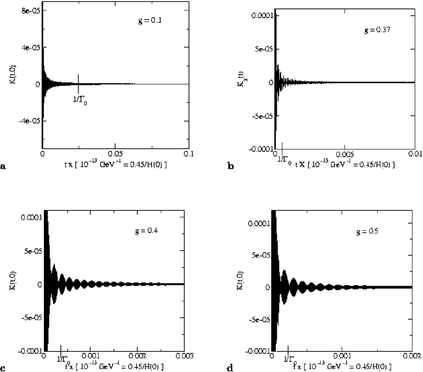
Figure 5: The kernel $K_{\chi}(t,0)$ of Eq. (105) for various interaction couplings $g$ and $h=g$, with $m_{\chi}=g\varphi(0)$, $\varphi(0)=m_{\rm Pl}$, $\lambda=10^{-13}$, and $\xi=0$.

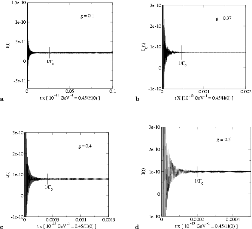
Figure 6: The integrated kernel $I_{\chi}(t,0)$ of Eq. (108) for various interaction couplings $g$ and $h=g$, with $m_{\chi}=g\varphi(0)$, $\varphi(0)=m_{\rm Pl}$, $\lambda=10^{-13}$, and $\xi=0$.

In Figs. 5 and 6, $K_{\chi}(t,0)$ and $I_{\chi}(t)$ respectively are plotted for the cases $g=0.1,0.37,0.4$ and $0.5$ in frames a-d respectively. In all the graphs the time interval $1/\Gamma_{0}(g)$ has been indicated, where $\Gamma_{0}(g)\equiv\Gamma_{\chi}(0)$ as defined in Eq. (98) is the $\chi$ decay width at zero momentum ${\bf q}=0$. The kernel $K_{\chi}(t,0)$ is seen to oscillate about zero with an overall enveloping amplitude that decays in a time interval $\sim 1/\Gamma_{\chi}$. The graphs of the integrated kernels $I_{\chi}(t)$, Fig. 6, show that there is an overall skewness, and within the time interval of order $1/\Gamma_{\chi}$, the integrated kernels converge to almost constant values. Thus, although the kernel does not have a simple Gaussian or exponential decay behavior, the rapid oscillatory behavior that it does have effectively causes it to retain memory only over a time interval of order $1/\Gamma_{\chi}$. It is also interesting to compare the kernel for the nonexpanding versus expanding cases, which is shown in Figs. 7 and 8 for $K_{\chi}(t,0)$ and $I_{\chi}(t)$ respectively at coupling $g=0.37$. The graphs show very little difference between the two cases, which was expected since $m_{\chi}\gg H$, and here is explicitly confirmed. For the parameters used in the figures we have that $m_{\chi}\gtrsim 10^{6}H$. What differences there are between the nonexpanding and expanding space-time kernels become increasingly pronounced as $t$ increases. This also is expected, since for very early times $t\ll 1/H$, the effect of expansion should be negligible. Note also in comparing Fig. 6 with Fig. 8 the y-axis is much more refined in the latter to help facilitate the desired comparison. However because of this in Fig. 8 the rapid decay of the integrated kernel below $t<1/\Gamma_{0}$ can not be seen.

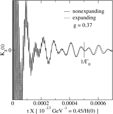
Figure 7: The kernel compared between the expanding Eq. (105) and nonexpanding cases for $g=h=0.37$, with $m_{\chi}=g\varphi(0)$, $\varphi(0)=m_{\rm Pl}$, $\lambda=10^{-13}$, and $\xi=0$.

Figure 8: The integrated kernel of Fig. 7 compared between the a. expanding and b. nonexpanding cases for $g=h=0.37$, with $m_{\chi}=g\varphi(0)$, $\varphi(0)=m_{\rm Pl}$, $\lambda=10^{-13}$, and $\xi=0$.

From the graphs of $I_{\chi}(t)$, the origin and validity of the local approximation Eq. (102) of the $\varphi$-evolution equation Eq. (83) can be understood. For this, first note that irrespective of the effects that dissipative damping have on slowing the evolution of $\varphi$, a minimal damping always arises from the $3H{\dot{\varphi}}$ term combined with the flatness of the potential, which in particular imply that within a time interval $\sim 1/H$, $\varphi$ and $\dot{\varphi}$ do not change significantly. In particular in integrating over the temporally nonlocal term in the $\varphi$-EOM Eq. (83) over a time interval of order $1/H$, $\varphi$ and $\dot{\varphi}$ can be treated as constant and so taken out of the time integration. This leaves integration over only $K_{\chi}(t,0)$ and as shown in Fig. 6, within a time interval $\sim 1/\Gamma_{\chi}$, this integral rapidly converges to an almost constant value, which is precisely $\Upsilon/\varphi^{2}$ of Eq. (103). Since $\Gamma_{\chi}\gg H$ in all the cases in Fig. 6 it also means $I_{\chi}(t)$ converges within a time $t\ll 1/H$.

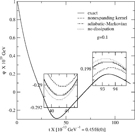
Figure 9: Evolution of $\varphi(t)$ for $g=h=0.1$, $\lambda=10^{-13}$, $\xi=0$, $\varphi(0)=m_{\rm Pl}$, and ${\dot{\varphi}}(0)=0$.

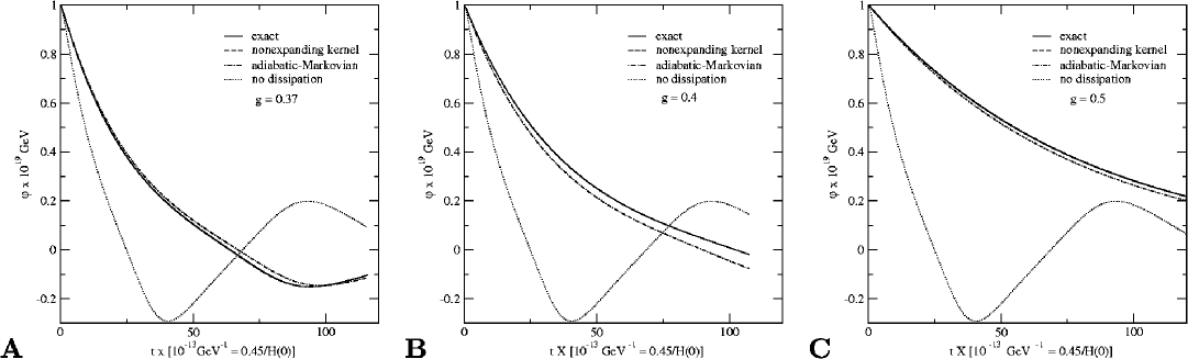
Figure 10: Evolution of $\varphi(t)$ for various interaction couplings $g$ and $h=g$, with $\lambda=10^{-13}$, $\xi=0$, $\varphi(0)=m_{\rm Pl}$, and ${\dot{\varphi}}(0)=0$.

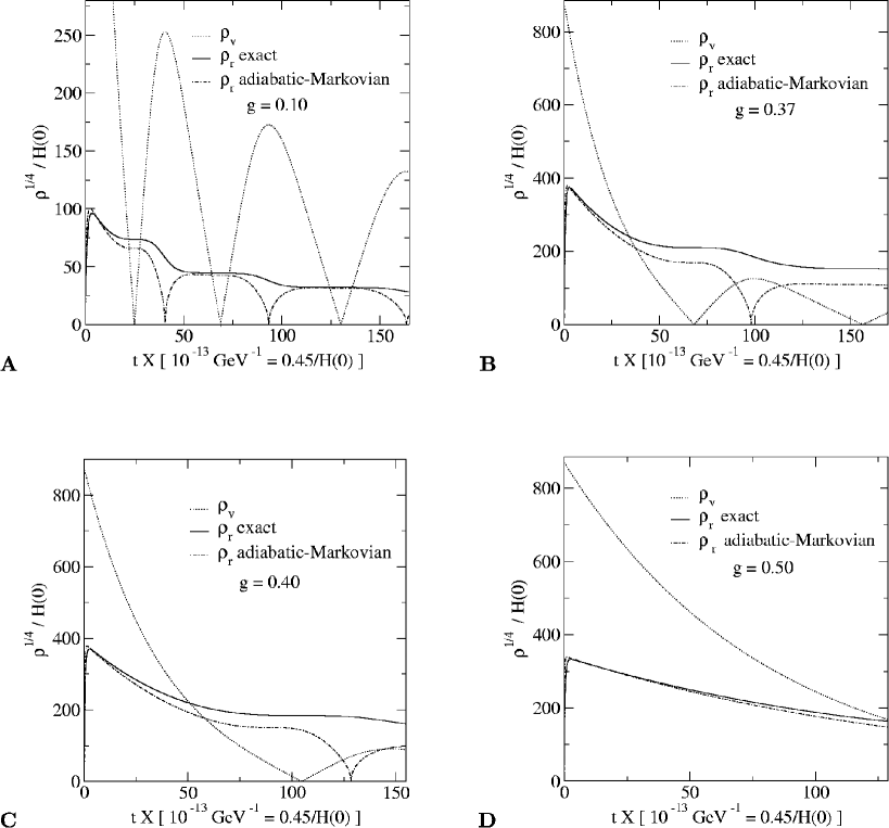
Figure 11: Evolution of radiation density $\rho_{r}$, plotted as the ratio $R\equiv\rho_{r}^{1/4}/H$ from various approximations and various interaction couplings $g$, with $h=g$, $\lambda=10^{-13}$, $\xi=0$, $\varphi(0)=m_{\rm Pl}$, and ${\dot{\varphi}}(0)=0$.

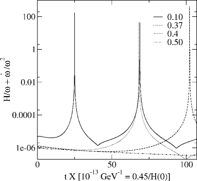
Figure 12: Checking the adiabatic approximation Eqs. (53), for various interaction couplings $g=0.1,0.37,0.4$ and $0.5$, with $h=g$, $\lambda=10^{-13}$, $\xi=0$, $\varphi(0)=m_{\rm Pl}$, and ${\dot{\varphi}}(0)=0$.

VI.2 $\varphi$ effective equation of motion

The solutions for $\varphi(t)$ from the effective evolution equation are plotted in Fig. 9 for $g=0.1$ and Fig. 10 frames a-c for $g=0.37,0.4$ and $0.5$, respectively. For each case the solution is plotted from the exact one-loop evolution equation Eq. (83) (solid), the same nonlocal evolution equation except with the kernel being replaced with its nonexpanding space-time counterpart (dashed), the adiabatic-Markovian evolution equation Eq. (102) (dot-dashed) and the evolution equation where no account for dissipative effects is treated (dotted). The latter dotted curves are the ones assumed in cold inflation studies, where the effects of dissipation are simply ignored. As Figs. 9 and 10 indicate, this assumption can be critically wrong. In particular, for the large coupling cases in Fig. 10, one sees that the effect of dissipation drastically affects the behavior of $\varphi(t)$ from the underdamped evolution found in the dotted curves to overdamped evolution once dissipative effects are properly accounted for. Comparing the three curves in each frame which treat dissipative effects at different levels of approximation, we see that they are all in excellent agreement. In particular, the adiabatic-Markovian approximation, which is based on the simplified evolution equation Eq. (102), is in excellent agreement with the exact evolution equation Eq. (83), where the nonlocal kernel is fully treated numerically. Based on our examination of the kernels in Figs. 5 and 6, and the fact that the integrated kernels rapidly converge in a time $t\ll 1/H$, these results for $\varphi(t)$ come as no surprise.

For the $g=0.37$ and $0.4$ cases, the longtime behavior appears to show oscillations as opposed to a complete overdamped relaxation. This is an artifact of our approximation of treating the $\varphi$-dependent $\chi$ field mass as fixed to the value of the field amplitude at the initial time $t_{0}$. This is done since then we can compute the kernel once and for all, before evolving $\varphi$ in Eq. (83). Allowing the $\chi$ mass to vary would require the kernel to be recomputed at every step of the evolution and that would be far too time consuming for this calculation be be tractable. However by doing this simplification, it leads to the nonlocal damping term depending on the field amplitude as $\varphi^{2}$ whereas itshould be $\varphi$. This means as $\varphi\rightarrow 0$, our approximation causes the nonlocal term to go to zero faster than it actually should and in particular faster than the curvature of the potential, thus leading to the oscillations. Thus for $g=0.37$ and $0.4$, the oscillations are simply an artifact of approximations used in numerically computing the $\varphi$ effective evolution equation.

Turning to Fig. 9 for $g=0.1$, we find that the effect of dissipation is not significant enough to alter the evolution of $\varphi(t)$ by very much. This is a weak dissipative regime, where in the adiabatic-Markovian approximation $\Upsilon<3H$. However the effect of dissipation is not entirely negligible. The two inset boxes in this figure close-up on $\varphi(t)$ at the two extrema. They show that the amplitude of $\varphi(t)$ is slightly less in the cases where dissipation is treated in comparison with the no dissipation (dotted curve) case. This indicates that energy is being depleted from the $\varphi$-system into radiation.

VI.3 Radiation production

In particular, Fig. 11 shows the ratio $\rho_{r}^{1/4}/H$ for the cases $g=0.1,0.37,0.4$ and $0.5$ in a-d respectively. In each frame there is a plot of $\rho_{r}$ from the exact evolution equations, Eqs. (83) and (91) (solid) and based on the adiabatic-Markovian evolution equations, Eqs. (102) and (104) (dashed). In all cases, the results show the exact and adiabatic-Markovian approximation are in good agreement. In particular, not only in the strong dissipative regime $\Upsilon>3H$ but also in the weak dissipative regime $\Upsilon<3H$, the simple formula Eq. (104) for determining radiation production is valid.

VI.4 Equilibration and thermalization: the asymptotic long time behavior

So far we have not discussed the long time behavior of our results, in particular the equilibration and thermalization of the radiation produced by the dissipation mechanism discussed in this paper. Before doing that it is useful to show whether and how our results, particularly the numerical ones given above for both the dissipative kernel and for the evolution of the $\varphi$ background field, can compare to recent numerical results obtained from the full evolution of fields far-from-equilibrium berges and therefore not restricted to quasi-equilibrium conditions only. Though here we have restricted our study of the dynamics for field configurations close to equilibrium and that evolve adiabatically, as we will see, our study still is able to capture many characteristics observed in the recent studies of the dynamics of scalar fields.

Recently the authors in berges have shown extensive numerical solutions for the kinetic (two-point correlation) equations for a scalar field in 1+1 D. Since these results seem also qualitatively to apply to 3+1 D, it is useful to see whether there is any similarity with the general characteristics observed for the dynamics, for both kernel and background field, obtained here compared to those obtained in berges . In particular, the authors of berges have shown that the dynamics of correlations (that also applies to the time dependent number density evolution) can generically be divided into three basic regimes: a damping regime characterized by an exponential suppression of the correlations in a time scale $t_{\rm damp}\sim 1/\Gamma$, followed by a drifting like evolution behavior characterized by smooth and slow changing of the modes, which typically lasts much longer than the initial damping evolution, after which a last regime sets in, the thermalization itself, in which thermal equilibrium is achieved, within a time scale $t_{\rm thermal}\gg t_{\rm damp}$. In the kinetic (or Boltzmann-like) approach in which the time evolution of correlations are solved, thermalization is seen as a direct consequence of self-consistently including scattering processes in the kinetic equations berges ; jakovac ; hu2 . In our case, this would be equivalent to self-consistently take into account in our evolution equation and in the derivation of the nonequilibrium propagators, the backreaction of the produced radiation. This is fundamental in order to describe the thermalization process, since in this way proper equipartition of energy among the modes is taken into account and that will then lead to thermal equilibration in the long time evolution of the system field. Therefore, our results will not account for the very long time thermalization regime. On the other hand, we can check from our numerical results, in particular for the temporal behavior for both the nonlocal dissipative kernel and also for its time integrated form, Figs. 5 and 6, respectively, that they show similar behavior to the correlations obtained by the authors in Ref. berges . In particular Figs. 5 and 6 show for the kernel a quick damping of oscillations within the time scale $1/\Gamma_{\chi}$, which is then followed by a drift like behavior of almost unperturbed, small amplitude oscillatory like evolution over a much larger time scale than $1/\Gamma_{\chi}$. Up to the time scales we have studied the dynamics, we have seen no appreciable change in this behavior. Thus the way our kernel evolves with these two regimes is analogous to those observed in the full kinetic equations approach of berges . This gives us an indication that, even though backreaction due to radiation production is not being fully taken into account, we are still capturing the relevant dynamics from the initial time of evolution (of no radiation) up to some very long time scale. Furthermore, it can be checked from the results shown in Fig. 11 that during the time scale of evolution that we have studied, the produced radiation maintains a level that is only a fraction of the inflaton energy density, $\rho_{r}/\rho_{\varphi}\lesssim 10^{-5}$, and, therefore, we expect its overall effect back on the evolution of the inflaton field to be only marginal.

The full inclusion of scattering and then the description of the final, asymptotic equilibration and thermalization regime, could in principle be done within the kinetic, Boltzmann-like approach of berges ; jakovac ; hu2 , or within other equivalent approaches able to describe the thermalization and equilibration process such as koide ; boyareheat . The extension of these approaches to our expanding space-time multifield setting is an interesting (and likely most more complex) avenue for future work, but it is beyond the scope of this paper.

VI.5 Adiabatic and WKB approximations

Finally we come to the analysis of some of our basic approximations used to derive the $\varphi$-EOM in its different forms. In Fig. 12 the validity of the adiabatic approximation is examined. From Eq. (53), recall this approximation is valid when $H/{\omega}+{\dot{\omega}}/{\omega^{2}}\ll 1$ (y-axis in the figure). For $g=0.5$, Fig. 10 shows that $\varphi$ remains overdamped throughout evolution and correspondingly Fig. 12 shows the adiabatic approximation remains excellent. However for $g=0.1,0.37$ and $0.4$ there are peaks crossing above one in Fig. 12, thus meaning the adiabatic approximation breaks down in those regions. In comparing to Figs. 9 and 10, all these peaks correspond to when the $\varphi(t)$ evolution seizes to be overdamped and it goes through a maxima or minima. In these underdamped regimes, in any event the dissipative term has no significant influence on the evolution of the system and so the breakdown of this approximation is of little consequence. Moreover, in the context of inflation, for $g=0.37$ and $0.4$ these breakdown regimes first occur at very late stages near the end of inflation, and so are not in a regime of interest for large scale structure formation. Also as commented earlier, in order to make our calculation tractable on the computer, we treated the $\varphi$-dependent $\chi$ field mass as fixed to the value of the field amplitude at the initial time $t_{0}$. This was done since then we can compute the kernel once and for all, before evolving $\varphi$ in Eq. (83), and thus cutting computation time by well over an order of magnitude and so bringing the computation time in the range of days as opposed to weeks. However by doing this simplification, it leads to the nonlocal damping term depending on the field amplitude as $\varphi^{2}$ whereas it should be $\varphi$. This means as $\varphi\rightarrow 0$, our approximation causes the nonlocal term to go to zero faster than it actually should and in particular faster than the curvature of the potential, thus leading to the oscillations. Thus for $g=0.37$ and $0.4$, the oscillations are simply an artifact of approximations used in numerically computing the $\varphi$ effective evolution equation. For $g=0.1$ the breakdown regimes of the adiabatic-Markovian approximation are real, however at early times, $t\lesssim 50$ in the units shown in Fig. 12, this approximation is excellent, so, for instance, results for radiation production at this time are reliable.

VII Dissipative Mechanism in Supersymmetry models

In the regimes where our dissipative mechanism is large enough to affect inflation, the interaction couplings also are significantly large to yield radiative corrections that harm the flatness of the inflaton effective potential. As such supersymmetry is needed, since it can cancel temporally local radiative effects from Bose and Fermi sectors, thus almost completely preserve the tree level potential. On the other hand, temporally nonlocal radiative effects, such as those that lead to dissipation, have very different space-time structure between Bose and Fermi sectors, and so are not canceled by SUSY.

As discussed in Sec. V.3, the $\psi_{\chi}$-fermions were included to mimic the effect of SUSY by cancelling the quantum corrections from the $\chi$-bosons. However the basic dissipative mechanism we have been studying in this paper, light boson (inflaton) $\rightarrow$ heavy boson $\rightarrow$ light fermions, can be realized in very simple SUSY models. For example, in Ref. BR3 we proposed the following model of two superfields $\Phi$ and $X$,

$$W=\frac{1}{3}\sqrt{\lambda}\Phi^{3}+g\Phi X^{2}+4mX^{2},$$ (109)

where $\Phi=\phi+\psi\theta+\theta^{2}F$ and $X=\chi+\theta\psi_{\chi}+\theta^{2}F_{\chi}$ are chiral superfields. The field $\phi$ will be identified as the inflaton in this model with $\phi=\varphi+\sigma$ and $\langle\phi\rangle=\varphi$. This is the simplest SUSY model in which the inflaton has a monomial potential, in this case

$$V_{0}(\varphi)=\frac{\lambda}{4}\varphi^{4},$$ (110)

and which includes the standard reheating interaction term to an additional boson $g^{2}\phi^{2}\chi^{2}$. When $\varphi\neq 0$ there is a nonzero vacuum energy and so SUSY is broken. This manifests in the splitting of masses between the $\chi$ and $\psi_{\chi}$ SUSY partners with in particular

$$m_{\psi_{\chi}}^{2} = \left[2g^{2}\varphi^{2}+16\sqrt{2}mg\varphi+64m^{2}\right]$$

$$m_{\chi_{1}}^{2} = \left[\frac{1}{8}(g^{2}+\frac{1}{2}\sqrt{\lambda}g)\varphi^{2}+\sqrt{2}mg\varphi+4m^{2}\right]=m^{2}_{\psi_{\chi}}+\sqrt{\lambda}g\varphi^{2}$$

$$m_{\chi_{2}}^{2} = \left[\frac{1}{8}(g^{2}-\frac{1}{2}\sqrt{\lambda}g)\varphi^{2}+\sqrt{2}mg\varphi+4m^{2}\right]=m^{2}_{\psi_{\chi}}-\sqrt{\lambda}g\varphi^{2}.$$ (111)

One can check that the one loop zero temperature effective potential correction in this case is not significant to alter the flatness of the tree level inflaton potential,

$$V_{1}(\varphi)\approx\frac{9}{128\pi^{2}}\lambda g^{2}\varphi^{4}\left[\ln\frac{m^{2}_{\psi_{\chi}}}{m^{2}}-2\right]\ll V_{0}(\varphi)=\frac{\lambda}{4}\varphi^{4}.$$ (112)

The authors of Ref. moss2 have recently studied independently the corrections in the model (109) including also the effect of finite temperature and reached analogous conclusion for the quantum corrections, that the $T=0$ and now also the thermal corrections can be kept under control. On the other hand this model has the interaction structure of the form Eq. (2), and so leads to the dissipative mechanism studied in this paper. In particular, one of the Yukawa couplings of this model is $4g\chi_{i}\psi_{\chi}\psi$. Noting the mass splittings in Eqs. (111), it means that the heavier $\chi$ boson, $\chi_{1}$ can decay into a $\psi_{\chi}$ fermion and an effectively massless inflatino $\psi$. There will be a phase space suppression in this process due to the closeness in masses of $\psi_{\chi}$ and $\chi_{1}$ so that the decay width now is

$$\Gamma_{\chi_{1}\rightarrow\psi_{\chi},\psi}=\frac{g\lambda}{4\sqrt{2}\pi}\varphi,$$ (113)

and this leads to the dissipative coefficient being

$$\Upsilon=\frac{\sqrt{2}g^{4}\lambda}{256\pi^{2}m_{\chi}}\varphi.$$ (114)

So in this case in general $\Gamma_{\chi_{1}\rightarrow\psi_{\chi},\psi},\Upsilon<H$. The radiation level, ${\cal R}$, during inflation is found from Eq. (104) to be

$${\cal R}\equiv\frac{\rho_{r}^{1/4}}{H}\approx 0.03\frac{g^{3/4}}{\lambda^{1/8}}\left(\frac{m_{\rm Pl}}{\varphi}\right)^{7/4}.$$ (115)

Thus for $\lambda=10^{-13}$ and $\varphi=m_{\rm Pl}$, ${\cal R}>1$ arises for $g>0.73$. However for $\varphi$ much larger than $m_{\rm Pl}$, ${\cal R}>1$ requires $g>1$. Thus this model is not very robust in producing radiation during inflation, but nevertheless the effect also is not negligible.

The radiation production during inflation in the model Eq. (109) can be greatly enhanced by adding some light fermions into which the $\chi_{i}$-bosons can decay. In any event, in a realistic particle physics model the inflaton sector, such as the model Eq. (109), would interact with other fields. This could be done for example with an another superfield $Y$ added to the superpotential Eq. (109) as $hXYY/2$, which leads to the Yukawa interaction term $h\chi\psi_{Y}\psi_{Y}$. Provided $2m_{Y}\ll m_{\chi}$, the $\chi$ decay width is unsuppressed and in particular would be just Eq. (97) with all other subsequent expressions there also applicable here. For this model we find in the strong dissipative regime $\Upsilon>3H$ that

$${\cal R}\equiv\frac{\rho_{r}^{1/4}}{H}\approx 2.66\frac{1}{g^{3/4}h^{1/2}\lambda^{1/8}}\left(\frac{m_{\rm Pl}}{\varphi}\right)^{5/4}.$$ (116)

For $\lambda=10^{-13}$ and $\varphi=5m_{\rm Pl}$, which in cold inflation analysis of this model would be approximately where the 60th e-fold of inflation occurs, we get ${\cal R}>1$ for $g^{3/2}h>0.09$. In the weak dissipative regime $\Upsilon<3H$ we find

$${\cal R}\equiv\frac{\rho_{r}^{1/4}}{H}\approx 0.036\frac{g^{3/4}h^{1/2}}{\lambda^{3/8}}\left(\frac{m_{\rm Pl}}{\varphi}\right)^{7/4},$$ (117)

for which ${\cal R}>1$ and the weak dissipation condition hold in the regime $0.00004<g^{3/2}h<0.09$. Thus warm inflation is very robust in this model.

VIII Influence of dissipation on density perturbations

Provided that the radiation component present during inflation is bigger than the inflaton mass, $\rho_{r}^{1/4}>m_{\phi}$, one should generally expect that this radiation component will influence the fluctuations of the inflaton. Since the typical mass of the inflaton is $\sim H$, this amounts to the criteria already mentioned in the Introduction $\rho_{r}^{1/4}>H$. Moreover, if one assumes thermalization, so that $\rho_{r}^{1/4}\approx T$, the inflaton fluctuations are then thermal. In this case the effect that the radiation component has on density fluctuations can be explicitly computed. Although it is beyond the scope of this paper to address the issue of thermalization, as a reasonable guideline thermalization is expected provided the decay width $\Gamma_{\chi}>H$. In this section, some examples of density perturbations during the warm inflation regime will be presented and the differences will be compared to the comparable results that would be obtained under the assumption of cold inflation.

For either ground state or thermal fluctuations of the inflaton, the density perturbations are obtained by the same expression Guth:ec ,

$$\delta_{H}=\frac{2}{5}\frac{H}{\dot{\varphi}}\delta\varphi\;.$$ (118)

In the warm inflation regime the fluctuations of the inflaton go in the strong dissipative regime as abadiab

$$\delta\varphi^{2}=\left(\frac{\pi}{4}\right)^{1/2}\sqrt{H\Upsilon}T\;,\;\;\;\;{\rm for\;warm\;inflation}\hskip 2.84544pt(\Upsilon>3H),\hskip 5.69046ptT>m_{\phi},$$ (119)

and in the the weak dissipative regime as Berera:1995wh

$$\delta\varphi^{2}=\left(\frac{3\pi}{4}\right)^{1/2}HT\;,\;\;\;\;{\rm for\;warm\;inflation}\hskip 2.84544pt(\Upsilon<3H),\hskip 5.69046ptT>m_{\phi}.$$ (120)

In contrast, for cold inflation, where inflaton fluctuations are exclusively quantum Guth:ec ,

$$\delta\varphi^{2}=\frac{H^{2}}{(2\pi)^{2}},\;\;\;\;\;{\rm for\;cold\;inflation},\hskip 5.69046ptT<m_{\phi}.$$ (121)

The associated spectral indices, $n_{s}$, for these three cases are Hall:2003zp

$$n_{s}-1\equiv\frac{d\ln\delta_{H}^{2}}{d\ln k}=\frac{1}{r}\left(-\frac{9}{4}\epsilon+\frac{3}{2}\eta-\frac{9}{4}\beta\right),\;\;\;\;\;{\rm for\;warm\;inflation}\hskip 2.84544pt(\Upsilon>3H),\hskip 5.69046ptT>m_{\phi},$$ (122)

$$n_{s}-1=\left(-\frac{17}{4}\epsilon+\frac{3}{2}\eta-\frac{1}{4}\beta\right),\;\;\;\;\;{\rm for\;warm\;inflation}\hskip 2.84544pt(\Upsilon<3H),\hskip 5.69046ptT>m_{\phi},$$ (123)

and spectrum

$$n_{s}-1=\left(-6\epsilon+2\eta\right),\;\;\;\;\;{\rm for\;cold\;inflation},\hskip 5.69046ptT<m_{\phi},$$ (124)

where $k$ is the wavenumber of the inflaton mode and the slow-roll parameters are defined as $\epsilon\equiv m_{p}^{2}V^{\prime 2}/(16\pi V^{2})$, $\eta\equiv m_{p}^{2}V^{\prime\prime}/(8\pi V)$, and $\beta\equiv m_{p}^{2}\Upsilon^{\prime}V^{\prime}/(8\pi\Upsilon V)$.

The spectral index will now be compared between the warm and cold inflation cases for the $\lambda\phi^{4}/4$ potential. For cold inflation the result are well known to be $n_{s}-1=-3/N_{3}$ spectrum , where $N_{e}$ denotes the number of e-folds of inflation. So at $N_{e}=60$, for example, $n_{s}-1=-1/20$, with the model parameters $\lambda=8\times 10^{-14}$ and $\varphi_{60}=4.37m_{\rm Pl}$. These parameters correspond to the amplitude of the density perturbations of $\delta_{H}\approx 10^{-5}$.

Turning to the warm inflation case, we now consider this potential coupled to additional fields in the manner of the Lagrangian Eq. (6) and account for the effects of radiation on density perturbations given by Eqs. (119) and (120). In this case for the same model parameters and this same value $\varphi_{60}$ of the field amplitude, these thermal effects increase the density perturbation normalization in the strong dissipative regime to $1\times 10^{-3}$. Thus the effect of dissipation and radiation production during inflation lead to a noticeable change in the behavior of the inflaton and its fluctuations. We now readjust the model parameters to properly normalize the density perturbations to the same value as before so that at $N_{e}\approx 60$, $\delta_{H}\approx 10^{-5}$. Nevertheless the spectral index will still differ. In particular normalizing the density perturbations as before requires the parameters in the strong dissipative regime to now be $\lambda\sim 10^{-17}$ and the spectral index at 60-efolds becomes $n_{s}-1=-1.5/N_{e}$. So for $N_{e}=60$ this implies in the strong dissipative warm inflation regime the $\lambda\phi^{4}/4$ potential leads to $n_{s}-1=0.025$ which is half the size of the correspond cold inflation result. Since the recent CMB satellite experiments, WMAP and upcoming Planck, should be able to discriminate spectral indices at the one percent level, the difference between warm and cold inflation might be detectable. This Section was simply illustrating some points regarding density perturbation differences in warm versus cold inflation. A detailed analysis of this issue will be presented in bb .

IX Conclusion

In this paper we have developed a formalism for treating dissipation in quantum field theory models with slowly evolving backgrounds in an expanding spacetime. The key steps for doing this were first computing the real-time matrix of dressed expanding space-time two-point Green’s functions for the respective quantum fields in our system. The solution of these Green’s functions was obtained in a WKB approximation, which is valid for slow moving evolution of the background fields and for fields with masses much bigger than the Hubble scale. Having derived these Green’s functions, we then used a standard response theory approximation approach for the derivation of the field averages appearing in the effective evolution equation for the background component of a scalar field $\varphi\equiv\langle\Phi\rangle$. The integration of the quantum field fluctuations employed a nonperturbative resummation. The resulting effective evolution equation for the background field $\varphi$ showed dissipative features.

As seen, our dissipative formalism differs from those used in treatments of reheating after inflation. In those cases, one is studying a fast moving, oscillating background component, typically in a linear relaxation (small field amplitude) regime. In contrast our analysis is applicable for slowly moving background fields that do not oscillate and in the nonlinear regime for the system field (the inflaton). As shown in Sec. II, the basic physics that underlies the dissipation in the two cases are markedly different. We have applied the nonlinear dissipative mechanism developed here to the inflationary regime. However, this same dissipation mechanism could also apply to preheating scenarios (if they are allowed by the model and given set of parameters), where the linearized, perturbative approximation for the inflaton breaks down and nonlinear, nonperturbative effects, such as the one studied in this paper, become important.

In addition to deriving the basic equations for our dissipative formalism, a detailed numerical analysis was done. In particular, the key quantity that our formalism determines is temporally nonlocal terms that must be included in the $\varphi$ background field effective evolution equation. In Sec. VI these nonlocal kernels were numerically calculated and compared at various levels of approximations. For instance, the $\varphi$ effective EOM was computed with the exact one-loop expression in Eq. (83). A key question was the regime of validity of the simplified adiabatic-Markovian approximation Eq. (102) to the exact equation. In Figs. 9 and 10 these comparisons were made. In the regime where the WKB self consistency conditions Eq. (53), together with the condition $\Gamma_{\chi_{j}}>H$ are satisfied, we found in Figs. 9 and 10 that the evolution equation computed from the exact one-loop expression and from the adiabatic-Markovian approximation agree very well within the region of parameters we have concentrated our study. We also checked in Sec. VI the radiation production from the $\varphi$ system that emerges through dissipation. Once again the exact numerical treatment and the adiabatic-Markovian approximation agreed very well in the same regimes as for the evolution equation. These results are of great practical use, since calculating the exact numerical solution to the effective evolution equation is very time consuming on the computer, whereas the evolution equation in the adiabatic-Markovian approximation can be analyzed analytically.

The immediate application of our dissipative formalism is to inflationary cosmology, in particular to determine warm inflation regimes and their properties. In Secs. VII and VIII we examined some consequences. In general there are two sorts of qualitative effects that dissipation can have on the inflationary phase. First, the evolution of the background field can be altered due to the nonlocal terms. The most dramatic example of that was shown in Fig. 10 where accounting for dissipation, $\varphi$ evolution was overdamped, whereas if one simply ignored these effects, the evolution would have the underdamped oscillatory behavior typically assumed in cold inflation studies. In particular, in the larger perturbative coupling regimes studied in Fig. 10, the inflaton field would never have a reheating phase (in the sense of a fast oscillatory like regime for $\varphi$). It would simply relax to the minimum of the potential monotonically, dissipating radiation along the way, thus ending the inflation phase and initiating a radiation dominated phase. Less dramatic to this, but down to much lower interaction couplings, even though the background inflaton field evolution is not noticeably altered from dissipative effects, radiation is still being produced during inflation from conversion of vacuum energy. Although there are detailed questions about thermalization, that are beyond the scope of this paper to address, as a reasonable criteria when $\rho_{r}^{1/4}>H$ during inflation, one should expect that this radiation component will influence the inflaton fluctuations significantly from its zero-temperature zero-point level. To gain a better understanding of the extent that this radiation can influence the inflaton fluctuations, and hence the primordial seeds of density fluctuations, in Sec. VIII we computed the density perturbations when the radiation component is accounted for, and compared that to the naive expectation when the fluctuations are assumed to be zero-point ground state fluctuations.

The key result of this study when applied to inflation has been that dissipative effects are predicted to occur during inflation in typical inflation models. These effects alter the single picture of inflationary dynamics assumed up to now, which we call cold inflation, into another possibility which we call warm inflation. To make accurate predictions from inflation models, which is now required for current high-precision CMB measurements, these dissipative effects must be treated. Moreover, dissipation effects can lead to some attractive theoretical consequences in inflation models. For example, for those parameter regions feasible to inflation and where the nonlinear and nonperturbative effects we studied here can become important, the emergence of effective strong dissipative phenomena are able, for instance, to sustain and drive inflation longer than when these dynamical effects are neglected ROR_pascos . Several other results also can follow as a consequence of the dissipative regimes studied here. In particular various problems, namely $\eta$ Berera:2004vm , graceful exit wi , quantum-to-classical transition wi ; Bellini:ki , large inflaton amplitude Berera:2004vm , and aspects of initial conditions bg ; ROR , can be remedied simply by properly accounting for the dissipative effects already in the model, rather than relying on additional modifications to the model, as is often done.

Appendix A The effective Potential and Renormalization

Consider the local terms (80) appearing in the $\varphi$-effective EOM and associated to the field derivative of the effective potential for $\varphi$,

$$\frac{\partial V_{\rm eff}(\varphi,R)}{\partial\varphi} = m_{\phi}^{2}\varphi(t)+\frac{\lambda}{6}\varphi(t)^{3}+\xi R(t)\varphi(t)$$ (125)

$$+ \frac{\lambda}{2}\varphi(t)\frac{1}{a(t)^{3}}\int\frac{d^{3}q}{(2\pi)^{3}}\frac{1}{2\left[{\bf q}^{2}/a(t)^{2}+m_{\phi}^{2}+\frac{\lambda}{2}\varphi(t)^{2}+(\xi-1/6)R(t)\right]^{1/2}}$$

$$+ \sum_{j=1}^{N_{\chi}}g_{j}^{2}\varphi(t)\frac{1}{a(t)^{3}}\int\frac{d^{3}q}{(2\pi)^{3}}\frac{1}{2\left[{\bf q}^{2}/a(t)^{2}+m_{\chi_{j}}^{2}+g_{j}^{2}\varphi(t)^{2}+(\xi-1/6)R(t)\right]^{1/2}}\;,$$

where we used Eqs. (78) and (79). The momentum integrals in Eq. (125) are divergent and require appropriate renormalization, which we perform here just as in standard Minkowski space-time. In Eq. (125) we add mass and couplings renormalization counterterms to the classical potential so as

$$\frac{\partial V_{\rm eff}(\varphi,R)}{\partial\varphi}\to\frac{\partial V_{\rm eff}(\varphi,R)}{\partial\varphi}+\delta m_{\phi}^{2}\varphi(t)+\frac{\delta\lambda}{6}\varphi(t)^{3}+\delta\xi R(t)\varphi(t)\;,$$ (126)

and we will consider from now on the masses and coupling constants as being the renormalized ones. The counterterms $\delta m_{\phi}^{2}$, $\delta\xi$ and $\delta\lambda$ are fixed by the choice of renormalization conditions ringwald ; ringwald2 )

$$\frac{\partial^{2}V_{\rm eff}(\varphi,R)}{\partial\varphi^{2}}\Bigr{|}_{\varphi=0,R=0}=m_{\phi}^{2}\;,$$

$$\frac{\partial^{3}V_{\rm eff}(\varphi,R)}{\partial R\partial\varphi^{2}}\Bigr{|}_{\varphi=0,R=\mu_{R}^{2}}=\xi\;,$$

$$\frac{\partial^{4}V_{\rm eff}(\varphi,R)}{\partial\varphi^{4}}\Bigr{|}_{\varphi=\mu_{\varphi},R=0}=\lambda\;,$$ (127)

where we have chosen renormalization points $\varphi=\mu_{\varphi}$ and $R=\mu_{R}^{2}$ in the above conditions so that the results are infrared finite in the limit of vanishing masses $m_{\phi}$ and $m_{\chi_{j}}$. Of course, these renormalization points are completely arbitrary and related to different choices by the corresponding renormalization group equations.

Using an upper momentum cutoff $\Lambda$ and changing to the physical momentum $k_{p}=k/a$ and cutoff $\Lambda_{p}=\Lambda/a$, the momentum integrals in Eq. (125) are easily evaluated leading to (for $\Lambda\to\infty$)

$$\frac{\partial V_{\rm eff}(\varphi,R)}{\partial\varphi} = (m_{\phi}^{2}+\delta m_{\phi}^{2})\varphi(t)+\frac{(\lambda+\delta\lambda)}{6}\varphi(t)^{3}+(\xi+\delta\xi)R(t)\varphi(t)$$ (128)

$$+ \left[\frac{\lambda}{2}+\sum_{j}g_{j}^{2}\right]\frac{\varphi}{8\pi^{2}}\Lambda_{p}^{2}+\frac{\lambda\varphi}{32\pi^{2}}\left[m_{\phi}^{2}+\frac{\lambda}{2}\varphi^{2}+\left(\xi-\frac{1}{6}\right)R\right]\left\{1+\ln\left[\frac{m_{\phi}^{2}+\frac{\lambda}{2}\varphi^{2}+\left(\xi-\frac{1}{6}\right)R}{4\Lambda_{p}^{2}}\right]\right\}$$

$$+ \sum_{j}\frac{g_{j}^{2}\varphi}{16\pi^{2}}\left[m_{\chi_{j}}^{2}+g_{j}^{2}\varphi^{2}+\left(\xi-\frac{1}{6}\right)R\right]\left\{1+\ln\left[\frac{m_{\chi_{j}}^{2}+g_{j}^{2}\varphi^{2}+\left(\xi-\frac{1}{6}\right)R}{4\Lambda_{p}^{2}}\right]\right\}\;.$$

We can now use the renormalization conditions (127) in (128) leading, for massless bare fields $m_{\phi}=m_{\chi_{j}}=0$, to the renormalized expression

$$\frac{\partial V_{\rm eff}^{r}(\varphi,R)}{\partial\varphi} = \frac{\lambda}{6}\varphi(t)^{3}+\xi R(t)\varphi(t)-\frac{\lambda}{32\pi^{2}}\left(\xi-\frac{1}{6}\right)R\varphi\left\{1+\ln\left[\frac{\left(\xi-\frac{1}{6}\right)\mu_{R}^{2}}{\frac{\lambda}{2}\varphi^{2}+\left(\xi-\frac{1}{6}\right)R}\right]\right\}$$ (129)

$$- \sum_{j}\frac{g_{j}^{2}}{16\pi^{2}}\left(\xi-\frac{1}{6}\right)R\varphi\left\{1+\ln\left[\frac{\left(\xi-\frac{1}{6}\right)\mu_{R}^{2}}{g_{j}^{2}\varphi^{2}+\left(\xi-\frac{1}{6}\right)R}\right]\right\}$$

$$- \frac{\lambda^{2}}{64\pi^{2}}\varphi^{3}\left\{\frac{11}{3}+\ln\left[\frac{\frac{\lambda}{2}\mu_{\varphi}^{2}}{\frac{\lambda}{2}\varphi^{2}+\left(\xi-\frac{1}{6}\right)R}\right]\right\}$$

$$- \sum_{j}\frac{g_{j}^{4}}{16\pi^{2}}\varphi^{3}\left\{\frac{11}{3}+\ln\left[\frac{g_{j}^{2}\mu_{\varphi}^{2}}{g_{j}^{2}\varphi^{2}+\left(\xi-\frac{1}{6}\right)R}\right]\right\}\;.$$

We can also extend the result for the renormalized effective potential when there is an additional coupling of $\Phi$ to fermions $\psi_{\chi}$, in which case there is the additional contribution to (125)

$$\frac{\partial V_{\rm eff}(\varphi,R)}{\partial\varphi}\to\frac{\partial V_{\rm eff}(\varphi,R)}{\partial\varphi}-\sum_{k}4h_{k}(m_{\psi}+h_{k}\varphi)\int\frac{d^{3}k_{p}}{(2\pi)^{3}}\frac{1}{2\sqrt{{\bf k}^{2}+(m_{\psi}+h_{k}\varphi)^{2}}}\;,$$ (130)

which leads to the additional contribution to (129) (for bare massless $\psi_{\chi}$ fermions, $m_{\psi}=0$)

$$\frac{\partial V_{\rm eff}^{r}(\varphi,R)}{\partial\varphi}\to\frac{\partial V_{\rm eff}^{r}(\varphi,R)}{\partial\varphi}+\sum_{k}\frac{h_{k}^{4}\varphi^{3}}{4\pi^{2}}\left(\frac{11}{3}+\ln\frac{\mu_{\varphi}^{2}}{\varphi^{2}}\right)\;.$$ (131)

References

- (1) A. Berera, M. Gleiser and R. O. Ramos, Phys. Rev. D58, 123508 (1998).
- (2) A. Berera, M. Gleiser and R. O. Ramos, Phys. Rev. Lett. 83, 264 (1999).
- (3) A. Berera and R. O. Ramos, Phys. Rev. D63, 103509 (2001).
- (4) A. Berera and R. O. Ramos, Phys. Lett. B567, 294 (2003).
- (5) A. Berera and R. O. Ramos, In Press Physics Letters B, arxiv: hep-ph/0308211, (2005).
- (6) A. H. Guth, Phys. Rev D23, 347 (1981); K. Sato, Phys. Lett. B99, 66 (1981).
- (7) A. Albrecht and P. J. Steinhardt, Phys. Rev. Lett. 48, 1220 (1982); A. Linde, Phys. Lett. 108B, 389 (1982).
- (8) A. Linde, Phys. Lett. 129B, 177 (1983).
- (9) A. Berera, Phys. Rev. Lett. 75, 3218 (1995); Phys. Rev. D54, 2519 (1996); Phys. Rev. D55, 3346 (1997).
- (10) H. P. de Oliveira and R. O. Ramos, Phys. Rev. D57, 741 (1998); W. Lee and L.-Z. Fang, Phys. Rev. D59, 083503 (1999).
- (11) L. F. Abbott, E. Fahri and M. Wise, Phys. Lett. 117B, 29 (1982).
- (12) L. Kofman, A. Linde and A. A. Starobinsky, Phys. Rev. D 56, 3258 (1997); P. B. Greene and L. Kofman, Phys. Lett. B448, 6 (1999); F. Finelli and R. Brandenberger, Phys. Rev. D62, 083502 (2000);
- (13) H. A. Weldon, Phys. Rev. D 28, 2007 (1983).
- (14) U. Weiss, Quantum Dissipative Systems (World Scientific, Singapure, 1999).
- (15) D. Boyanovsky, H. J. de Vega, R. Holman, D.-S. Lee and A. Singh, Phys. Rev. D51, 4419 (1995).
- (16) M. Gleiser and R. O. Ramos, Phys. Rev. D50, 2441 (1994).
- (17) N. Banerjee and S. Mallik, Phys. Rev. D45, 701 (1992).
- (18) K. Chou, Z. Su, B. Hao and L. Yu, Phys. Rep. 118, 1 (1985); N. P. Landsman and Ch. G. van Weert, Phys. Rep. 145, 141 (1987).
- (19) I. D. Lawrie, J. Phys. A25, 6493 (1992); Phys. Rev. D60, 063510 (1999).
- (20) S. A. Ramsey, B. L. Hu and A. M. Stylianopoulos, Phys. Rev. D 57, 6003 (1998).
- (21) N. D. Birrel and P. C. W. Davis, Quantum Fields in Curved Space (Cambridge University Press, Cambridge, England, 1982); S. A. Fulling, Aspects of Quantum Field Theory in Curved Space Time (Cambridge University Press, Cambridge, England, 1989).
- (22) G. Semenoff and N. Weiss, Phys. Rev. D31, 699 (1985).
- (23) H. Leutwyler and S. Mallik, Ann. Phys. (NY) 205, 1 (1991).
- (24) S. Habib, Phys. Rev. D46, 2408 (1992).
- (25) R. H. Brandenberger, S. E. Joras and J. Martin, Phys. Rev. D66, 083514 (2002); J. Martin and R. H. Brandenberger, Phys. Rev. D67, 083512 (2003).
- (26) A. Ringwald, Ann. Phys. (NY) 177, 129 (1987).
- (27) I. D. Lawrie, Phys. Rev. D67, 045006 (2003).
- (28) G. Aarts and J. Berges, Phys. Rev. D 64, 105010 (2001).
- (29) A. L. Fetter and J. D. Walecka, Quantum Theory of Many Particle Systems (McGraw-Hill, New York, 1971).
- (30) A. Ringwald, Phys. Rev. D36, 2598 (1987).
- (31) A. Vilenkin, Nucl. Phys. B 226, 504 (1983).
- (32) D. Boyanovsky, R. Holman and S. Prem Kumar, Phys. Rev. D56, 1958 (1997); D. Boyanvsky and H. J. de Vega, arXiv: astro-ph/0406287.
- (33) J. Berges and J. Cox, Phys. Lett. B517, 369 (2001); J. Berges, Nucl. Phys. A699, 847 (2002).
- (34) A. Jakovac, Phys. Rev. D 65, 085029 (2002).
- (35) E. Calzetta and B. L. Hu, Phys. Rev. D 61, 025012 (2000).
- (36) T. Koide and M. Maruyama, Nucl. Phys. A742, 95 (2004); T. Koide, Prog. Theor. Phys. 107, 525 (2002).
- (37) D. Boyanovsky, M. D’attanasio, H. J. de Vega, R. Holman and D.-S. Lee, Phys. Rev. D 52, 6805 (1995); D. Boyanovsky, I. D. Lawrie, D. S. Lee, Phys. Rev. D 54, 4013 (1996).
- (38) L. M. H. Hall and I. G. Moss, arXiv: hep-ph/0408323.
- (39) A. H. Guth and S. Y. Pi, Phys. Rev. Lett. 49, 1110 (1982).
- (40) A. Berera, Nucl. Phys. B585, 666 (2000).
- (41) A. Berera and L. Z. Fang, Phys. Rev. Lett. 74, 1912 (1995).
- (42) L. M. H. Hall, I. G. Moss and A. Berera, Phys. Rev. D 69, 083525 (2004).
- (43) A. R. Liddle and D. H. Lyth, Phys. Lett. B 291, 391 (1992).
- (44) M. Bastero-Gil and A. Berera, In Press Physical Review D, hep-ph/0411144, (2005).
- (45) R. O. Ramos, arXiv: hep-ph/0409353.
- (46) A. Berera, arXiv:hep-ph/0401139.
- (47) M. Bellini, Phys. Lett. B 428, 31 (1998).
- (48) A. Berera and C. Gordon, Phys. Rev. D63, 063505 (2001).
- (49) R. O. Ramos, Phys. Rev. D64, 123510 (2001).