IFIC/04-32
RBRC-422
BNL-NT-04/22
Collinear splitting, parton evolution and the strange-quark asymmetry of the nucleon in NNLO QCD

Abstract

We consider the collinear limit of QCD amplitudes at one-loop order, and their factorization properties directly in colour space. These results apply to the multiple collinear limit of an arbitrary number of QCD partons, and are a basic ingredient in many higher-order computations. In particular, we discuss the triple collinear limit and its relation to flavour asymmetries in the QCD evolution of parton densities at three loops. As a phenomenological consequence of this new effect, and of the fact that the nucleon has non-vanishing quark valence densities, we study the perturbative generation of a strange–antistrange asymmetry $s(x)-\bar{s}(x)$ in the nucleon’s sea.

1 INTRODUCTION

The high precision of experiments at past, present and future particle colliders (LEP, HERA, Tevatron, LHC, $e^{+}e^{-}$ linear colliders) demands a corresponding precision in theoretical predictions. As for perturbative QCD predictions, this means calculations beyond the next-to-leading order (NLO) in the strong coupling $\alpha_{\mathrm{S}}$. Recent years have witnessed much progress in this field. In particular, a great deal of work has been devoted to study the properties of QCD scattering amplitudes in the infrared (soft and collinear) region [1]–[12].

The understanding of the infrared singular behaviour of QCD amplitudes is a prerequisite for the evaluation of infrared-finite cross sections (and, more generally, infrared- and collinear-safe QCD observables) at higher orders in perturbation theory. Moreover, the information on the infrared properties of the amplitudes can be exploited to compute large (logarithmically enhanced) perturbative terms and to resum them to all perturbative orders [13]. Those investigations are also valuable for improving the physics content of Monte Carlo event generators (see e.g. Ref. [14]). In addition, these studies prove to be useful even beyond the strict QCD context, and can provide hints on the structure of highly symmetric gauge theories at infinite orders in the perturbative expansion (e.g. N=4 super-Yang-Mills, see Ref. [15]).

Another important application is the calculation of the Altarelli–Parisi (AP) kernels, that control the scale evolution of parton densities and fragmentation functions. The calculation of the next-to-next-to-leading order (NNLO) kernels has been completed very recently [16]. Collinear factorization at the amplitude level (see Sect. 2) can be used [17] as an alternative and independent method to perform that calculation. To this purpose, the one-loop triple collinear splitting [11] (see Sect. 3) is one of the necessary ingredients. Two other ingredients are the tree-level quadruple collinear splitting [8] and the two-loop double collinear splitting [12].

Besides increasing the quantitative precision of the theoretical calculations, the evaluation of higher-order contributions can reveal qualitatively new quantum effects. An interesting example is the perturbative generation of charge asymmetries in the nucleon’s sea [18] (see Sect. 4), which arises from the NNLO evolution of parton densities.

2 COLLINEAR FACTORIZATION IN COLOUR SPACE

We consider a generic scattering process involving final-state QCD partons (massless quarks and gluons) of flavour $a_{1},a_{2},\dots$ and momenta $p_{1},p_{2},\dots$, which is described by the matrix element ${\cal M}_{a_{1},a_{2},\dots}(p_{1},p_{2},\dots)$; the external legs are on shell $(p_{i}^{2}=0)$ and have physical spin polarizations. Up to one-loop order, one can write

$${\cal M}=\left(g_{\mathrm{S}}\right)^{q}\;\left[\;{\cal M}^{(0)}+\frac{\alpha_{\mathrm{S}}}{2\pi}\;{\cal M}^{(1)}+{\cal O}(\alpha_{\mathrm{S}}^{2})\right]~{},$$ (1)

where the overall power $q$ is integer. The one-loop amplitude ${\cal M}^{(1)}$ contains ultraviolet and infrared singularities that are regularized by using dimensional regularization in $d=4-2\epsilon$ space-time dimensions ($\mu$ is the dimensional-regularization scale).

The multiple collinear limit is approached when the momenta $p_{1},\dots,p_{m}$ of $m$ partons become parallel. In this limit all the particle subenergies $s_{ij}=(p_{i}+p_{j})^{2}$, with $i,j=1,\dots,m$, are of the same order and vanish simultaneously, and the matrix element ${\cal M}(p_{1},\dots,p_{m},p_{m+1},\dots)$ becomes singular. At the tree level, the dominant singular behaviour is ${\cal M}^{(0)}(p_{1},\dots,p_{m},p_{m+1},\dots)\sim(1/{\sqrt{s}})^{m-1}$, where $s$ generically denotes a two-particle subenergy $s_{ij}$, or a three-particle subenergy $s_{ijk}$, and so forth. At one-loop order, this singular behaviour is simply modified by scaling violation, ${\cal M}^{(1)}(p_{1},\dots,p_{m},p_{m+1},\dots)\sim(1/{\sqrt{s}})^{m-1}(s/\mu^{2})^{-\epsilon}$. The dominant singular behaviour is captured by universal (process-independent) factorization formulae, that are usually presented upon decomposition in colour subamplitudes [5]–[9]. Collinear factorization is nonetheless valid directly in colour space [11].

Figure 1: Factorization of tree-level amplitudes in the multiple collinear limit.

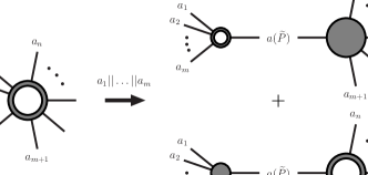
Figure 2: Factorization of one-loop amplitudes in the multiple collinear limit.

The colour-space factorization formulae for the multiple collinear limit of the tree-level and one-loop amplitudes ${\cal M}^{(0)}$ and ${\cal M}^{(1)}$ are:

$$|{{\cal M}_{a_{1},\dots,a_{m},a_{m+1},\dots}^{(0)}(p_{1},\dots,p_{m},p_{m+1},\dots)}\rangle\simeq$$ (2)

$${{\mbox{\boldmath$Sp$}}}_{a_{1}\dots a_{m}}^{(0)}(p_{1},\dots,p_{m})\;|{{\cal M}_{a,a_{m+1},\dots}^{(0)}({\widetilde{P}},p_{m+1},\dots)}\rangle~{},$$

$$|{{\cal M}_{a_{1},\dots,a_{m},a_{m+1},\dots}^{(1)}(p_{1},\dots,p_{m},p_{m+1}\dots)}\rangle\simeq$$ (3)

$${{\mbox{\boldmath$Sp$}}}_{a_{1}\dots a_{m}}^{(1)}(p_{1},\dots,p_{m})\;|{{\cal M}_{a,a_{m+1}\dots}^{(0)}({\widetilde{P}},p_{m+1},\dots)}\rangle+$$

$${{\mbox{\boldmath$Sp$}}}_{a_{1}\dots a_{m}}^{(0)}(p_{1},\dots,p_{m})\;|{{\cal M}_{a,a_{m+1},\dots}^{(1)}({\widetilde{P}},p_{m+1},\dots)}\rangle~{}.$$

These factorization formulae are valid in any number $d=4-2\epsilon$ of space-time dimensions. The only approximation involved on the right-hand sides amounts to neglecting terms that are less singular in the multiple collinear limit. A graphical representation of the factorization formulae is shown in Figs. 1 and 2. Equations (2) and (3) relate the original matrix element (on the left-hand side) with $m+k$ partons (where $k$ is arbitrary) to a matrix element (on the right-hand side) with $1+k$ partons. The latter is obtained from the former by replacing the $m$ collinear partons with a single parent parton, whose momentum ${\widetilde{P}}$ (${\widetilde{P}}^{2}=0$) defines the collinear direction and whose flavour $a$ is determined by flavour conservation in the splitting process $a\to a_{1}+\dots+a_{m}$. The derivation of Eq. (2) in colour space is quite straightforward [4]. Its one-loop extension, Eq. (3), follows, in particular, from colour coherence of QCD radiation [19].

The process dependence of the factorization formulae is entirely embodied in the matrix elements. The tree-level and one-loop factors ${{\mbox{\boldmath$Sp$}}}^{(0)}_{a_{1}\cdots a_{m}}$ and ${{\mbox{\boldmath$Sp$}}}^{(1)}_{a_{1}\cdots a_{m}}$, which encode the singular behaviour in the multiple collinear limit, are universal (process-independent). They depend on the momenta and quantum numbers (flavour, spin, colour) of the $m$ partons that arise from the collinear splitting. The splitting matrix ${{\mbox{\boldmath$Sp$}}}_{a_{1}\cdots a_{m}}$ is a matrix in colour+spin space, acting onto the colour and spin indices of the $m$ collinear partons on the left and onto the colour and spin indices of the parent parton on the right.

The square of the splitting matrix ${{\mbox{\boldmath$Sp$}}}_{a_{1}\cdots a_{m}}$, summed over final-state colours and spins and averaged over colours and spins of the parent parton, defines the $m$-parton splitting function $\langle\hat{P}_{a_{1}\cdots a_{m}}\rangle$, which is a generalization of the customary (i.e. with $m=2$) AP splitting function [20]. The normalization of the tree-level $\langle\hat{P}^{(0)}_{a_{1}\cdots a_{m}}\rangle$ and one-loop $\langle\hat{P}^{(1)}_{a_{1}\cdots a_{m}}\rangle$ splitting functions is fixed by

$$\langle\hat{P}_{a_{1}\cdots a_{m}}^{(0)}\rangle=\left(\frac{s_{1\dots m}}{2\;\mu^{2\epsilon}}\right)^{m-1}\;{\overline{|{{\mbox{\boldmath$Sp$}}}_{a_{1}\dots a_{m}}^{(0)}|^{2}}}~{},$$ (4)

$$\langle\hat{P}_{a_{1}\cdots a_{m}}^{(1)}\rangle=$$

$$\;\;\;\;\left(\frac{s_{1\dots m}}{2\;\mu^{2\epsilon}}\right)^{m-1}{\overline{\left[({{\mbox{\boldmath$Sp$}}}^{(0)}_{a_{1}\cdots a_{m}})^{\dagger}\,{{\mbox{\boldmath$Sp$}}}^{(1)}_{a_{1}\cdots a_{m}}+\mathrm{h.c.}\right]}}~{}.$$

The one-loop amplitude ${\cal M}^{(1)}$ and, hence, ${{\mbox{\boldmath$Sp$}}}^{(1)}$ have ultraviolet and infrared divergences that show up as $\epsilon$-poles in dimensional regularization. The one-loop splitting matrix can be decomposed as

$${{\mbox{\boldmath$Sp$}}}^{(1)}_{a_{1}\cdots a_{m}}={{\mbox{\boldmath$Sp$}}}^{(1)\,{\rm div.}}_{a_{1}\cdots a_{m}}+{{\mbox{\boldmath$Sp$}}}^{(1)\,{\rm fin.}}_{a_{1}\cdots a_{m}}~{},$$ (5)

where ${{\mbox{\boldmath$Sp$}}}^{(1)\,{\rm div.}}_{a_{1}\cdots a_{m}}$ contains all the $\epsilon$-poles and ${{\mbox{\boldmath$Sp$}}}^{(1)\,{\rm fin.}}_{a_{1}\cdots a_{m}}$ is finite when $\epsilon\to 0$. In Ref. [11] we have presented the explicit expression of ${{\mbox{\boldmath$Sp$}}}^{(1)\,{\rm div.}}_{a_{1}\cdots a_{m}}$ for an arbitrary number $m$ of final-state collinear partons.

3 ONE-LOOP TRIPLE COLLINEAR SPLITTING

The one-loop splitting amplitudes for the double collinear limit $a\to a_{1}+a_{2}$ are known [5, 6, 7]. As a first step beyond the double collinear limit, we have considered [11] the triple collinear splitting process $q\to q+\bar{q}^{\prime}+q^{\prime}$, where $q$ and $q^{\prime}$ denote quarks of different flavours. To evaluate the one-loop splitting matrix we have used a process-independent method [4, 7, 19]. Considering physical spin polarizations, the splitting matrix is calculated from the sole Feynman diagrams where the parent parton emits and absorbs collinear radiation. In the case $q\to q+\bar{q}^{\prime}+q^{\prime}$, one has to consider, for instance, the one-loop diagram depicted in Fig. 3(a).

Our computation of ${{\mbox{\boldmath$Sp$}}}^{(1)}$ requires the evaluation of a set of basic one-loop (scalar and tensor) integrals. Besides the customary one-loop integrals, new integrals with additional propagators of the type $1/(n\cdot q)$ ($q$ is the loop momentum and $n$ is an auxiliary light-like vector), which come from the physical polarizations of the virtual gluons, have to be calculated. Some of these integrals, which resemble those encountered in axial-gauge calculations, were evaluated in Ref. [7] in the context of the calculation of the one-loop double collinear splitting $a\to a_{1}+a_{2}$. More complicated integrals (higher-point functions) of this type are involved in triple collinear splitting processes. We have computed (to high orders in the $\epsilon$ expansion) all the basic one-loop integrals that appear in any triple collinear splitting. These results can be applied to evaluate the one-loop splitting matrix of any splitting process $a\to a_{1}+a_{2}+a_{3}$ [19].

The explicit expressions up to ${\cal O}(\epsilon^{0})$ of the splitting matrix ${{\mbox{\boldmath$Sp$}}}_{q\bar{q}^{\prime}q^{\prime}}$ and of the corresponding splitting function $\langle\hat{P}^{(1)}_{q\bar{q}^{\prime}q^{\prime}}\rangle$ (see Fig. 3(a)) are presented in Ref. [11]. It is important to observe that $\langle\hat{P}^{(1)}_{q\bar{q}^{\prime}q^{\prime}}\rangle$ has a contribution (which is proportional to the color factor $d^{abc}d_{abc}$) that changes sign by exchanging the momenta of the evolved quark and antiquark $q^{\prime}$ and $\bar{q}^{\prime}$. This charge asymmetry is a new quantum effect produced by the exchange of three gluons in the $t$-channel. When the charge asymmetry of $\langle\hat{P}^{(1)}_{q\bar{q}^{\prime}q^{\prime}}\rangle$ is combined with the corresponding tree-level contribution (see Fig. 3(b)), it leads to a non-vanishing value of the NNLO AP kernel $P_{qq^{\prime}}-P_{q\bar{q}^{\prime}}$. The main physical consequence of this effect is discussed in Sect. 4.

4 STRANGE-QUARK ASYMMETRY IN THE NUCLEON

Strange quarks and antiquarks play a fundamental role in the structure of the nucleon [21]. Among the various strangeness–related properties of the nucleon, the strange “asymmetry”, $s(x)-\bar{s}(x)$, in the densities of strange quarks and antiquarks, $x$ being the light-cone momentum fraction they carry, is of particular interest. Since the nucleon does not carry any strangeness quantum number, the integral of the asymmetry over all values of $x$ has to vanish:

$$\langle s-\bar{s}\rangle\equiv\int_{0}^{1}dx\,\left[s(x)-\bar{s}(x)\right]=0\;.$$ (6)

However, there is no symmetry that would prevent the $x$ dependences of the functions $s(x)$ and $\bar{s}(x)$ from being different. Therefore one can expect $s(x)\neq\bar{s}(x)$, in general.

Strange–antistrange asymmetries have been extensively discussed in the literature. Various non-perturbative models of the nucleon structure [22] predict a fairly small value of the second moment of the strange–antistrange distribution, $|\langle x(s-\bar{s})\rangle|\sim 10^{-4}$. A global analysis of unpolarized parton distributions [23] reported improvements in the data fit if the asymmetry $s(x)-\bar{s}(x)$ is positive at high $x$. However, a recent update [24] of this analysis reduces the asymmetry significantly. The most recent global QCD fit [25] finds a large uncertainty for that asymmetry and quotes a range $-0.001<\langle x(s-\bar{s})\rangle<0.004$. The strange asymmetry in the nucleon has become particularly relevant in view of the “anomaly” seen by the NuTeV collaboration in their measurement of the Weinberg angle [26]. The anomaly could be partly explained [27, 28] by a positive value of the second moment $\langle x(s-\bar{s})\rangle$.

Figure 3: Example of (a) virtual and (b) real contributions to $P_{ns}^{(2)S}$.

The discussion reported so far regards strange–antistrange asymmetries that are generated by non-perturbative mechanisms. Then, because of the customary scaling violation, the asymmetry becomes dependent on the hard-scattering scale $Q$ at which the nucleon is probed.

Perturbative QCD alone, however, definitely predicts a non-vanishing and $Q$-dependent value of the strange–antistrange asymmetry [18]. The effect arises because at NNLO in perturbation theory the probability of the inclusive collinear splitting (evolution) $q\to q^{\prime}$ becomes different from that of $q\to\bar{q}^{\prime}$, and because the nucleon has $u$ and $d$ valence densities.

Owing to charge conjugation invariance and flavour symmetry of QCD, the AP kernels that control the parton evolution of quark–antiquark asymmetries can be written as (see e.g. Ref. [29])

$$P_{q_{i}q_{j}}-P_{q_{i}\bar{q}_{j}} = P_{\bar{q}_{i}\bar{q}_{j}}-P_{\bar{q}_{i}q_{j}}$$ (7)

$$= \delta_{ij}\;P^{(-)}+(P_{qq^{\prime}}-P_{q\bar{q}^{\prime}})\;.$$

The AP kernels $P_{qq^{\prime}}$ and $P_{q\bar{q}^{\prime}}$ describe splittings in which the flavor of the quark changes, and $P_{qq^{\prime}}\neq P_{q\bar{q}^{\prime}}$ starting from NNLO [29, 30]. In particular, as discussed at the end of Sect. 3, $P_{qq^{\prime}}-P_{q\bar{q}^{\prime}}=(\alpha_{\mathrm{S}}/(4\pi))^{3}P_{ns}^{(2)S}/N_{f}$, because of the charge asymmetry produced by quantum effects at order $\alpha_{\mathrm{S}}^{3}$. The explicit expression of $P_{ns}^{(2)S}$ is now available thanks to the recent computation by Moch, Vermaseren and Vogt [16].

The solution of the AP equations for the evolution (between the scales $Q_{0}$ and $Q$) of the $N$-moment, $(s-{\bar{s}})_{N}=\langle x^{N-1}(s-{\bar{s}})\rangle$, of the strange-quark asymmetry reads [18]

$$\!\!\!\!\!\!\!\!\!\!\!\!\left(s-{\bar{s}}\right)_{N}(Q^{2})=U_{N}(Q,Q_{0})\;\big{[}\;\left(s-{\bar{s}}\right)_{N}(Q_{0}^{2})$$

$$+\,\delta P_{N}^{(2)}\left(\alpha_{\mathrm{S}}^{2}(Q)-\alpha_{\mathrm{S}}^{2}(Q_{0})\right)q^{(V)}_{N}(Q_{0}^{2})\;\big{]}~{},$$ (8)

where $q^{(V)}\equiv\sum_{i=1}^{N_{f}}(q_{i}-{\bar{q}}_{i})$ is the valence density of the nucleon, $U_{N}$ is the evolution operator controlled by $P^{(-)}$, and $\delta P_{N}^{(2)}$ is proportional to the NNLO kernel $P_{ns}^{(2)S}$ [18]. At LO and NLO, $\delta P_{N}^{(2)}=0$, and thus any asymmetry can only be produced by a corresponding asymmetry at the scale $Q_{0}$. Starting from NNLO, the degeneracy of $P_{qq^{\prime}}$ and $P_{q\bar{q}^{\prime}}$ is removed, and perturbative QCD necessarily predicts a non-vanishing $s-{\bar{s}}$ asymmetry driven by the valence density.

Predictions for $(s-{\bar{s}})(x,Q^{2})$ based on Eq. (4) have been presented in Ref. [18]. The asymmetry, $s-{\bar{s}}$, is set to zero at a given low scale $Q_{0}$, and then evolved upwards. The generated asymmetry is fairly sizable and turns out to be positive at small $x$ and negative at large $x$. Using $Q_{0}\sim 0.5$ GeV (as in the ‘radiative’ parton model analysis of Ref. [31]), a negative second moment is found:

$$\langle x(s-\bar{s})\rangle\approx-5\times 10^{-4}\;\;\;\;\;\;(Q^{2}=20\,\mathrm{GeV}^{2})~{}.$$ (9)

The analysis has also be extended [18] to predict the asymmetries of heavy flavours $c$ and $b$.

Acknowledgments: G.R. thanks S. Moch and J. Blümlein for their kind invitation to present these results at Zinnowitz, and for the pleasant organization of the workshop.

References

- [1] F. A. Berends and W. T. Giele, Nucl. Phys. B 313 (1989) 595.
- [2] S. Catani, Phys. Lett. B 427 (1998) 161; S. Catani and M. Grazzini, Nucl. Phys. B 591 (2000) 435.
- [3] J. M. Campbell and E. W. Glover, Nucl. Phys. B 527 (1998) 264.
- [4] S. Catani and M. Grazzini, Phys. Lett. B 446 (1999) 143, Nucl. Phys. B 570 (2000) 287.
- [5] Z. Bern, L. J. Dixon, D. C. Dunbar and D. A. Kosower, Nucl. Phys. B 425 (1994) 217.
- [6] Z. Bern, V. Del Duca and C. R. Schmidt, Phys. Lett. B 445 (1998) 168; Z. Bern, V. Del Duca, W. B. Kilgore and C. R. Schmidt, Phys. Rev. D 60 (1999) 116001.
- [7] D. A. Kosower, Nucl. Phys. B 552 (1999) 319; D. A. Kosower and P. Uwer, Nucl. Phys. B 563 (1999) 477.
- [8] V. Del Duca, A. Frizzo and F. Maltoni, Nucl. Phys. B 568 (2000) 211.
- [9] D. A. Kosower, Phys. Rev. D 67 (2003) 116003, Phys. Rev. Lett. 91 (2003) 061602, hep-ph/0311272.
- [10] G. Sterman and M. E. Tejeda-Yeomans, Phys. Lett. B 552 (2003) 48.
- [11] S. Catani, D. de Florian and G. Rodrigo, Phys. Lett. B 586 (2004) 323.
- [12] Z. Bern, L. J. Dixon and D. A. Kosower, hep-ph/0404293; S. D. Badger and E. W. N. Glover, hep-ph/0405236.
- [13] D. de Florian and M. Grazzini, Phys. Rev. Lett. 85 (2000) 4678, Nucl. Phys. B 616 (2001) 247; S. Catani, D. de Florian and M. Grazzini, JHEP 0105 (2001) 025; S. Catani, D. de Florian, M. Grazzini and P. Nason, JHEP 0307 (2003) 028.
- [14] CERN Workshop on Monte Carlo tools for the LHC, CERN, Geneva, July 2003.
- [15] C. Anastasiou, Z. Bern, L. J. Dixon and D. A. Kosower, Phys. Rev. Lett. 91 (2003) 251602.
- [16] S. Moch, J. A. M. Vermaseren and A. Vogt, Nucl. Phys. B 688 (2004) 101, hep-ph/0404111.
- [17] D. A. Kosower and P. Uwer, Nucl. Phys. B 674 (2003) 365.
- [18] S. Catani, D. de Florian, G. Rodrigo and W. Vogelsang, hep-ph/0404240.
- [19] S. Catani, D. de Florian, G. Rodrigo and W. Vogelsang, in preparation.
- [20] G. Altarelli and G. Parisi, Nucl. Phys. B 126 (1977) 298.
- [21] J. R. Ellis, Nucl. Phys. A684 (2001) 53.
- [22] G. Cao and A. I. Signal, Phys. Rev. D 60 (1999) 074021, and references therein.
- [23] V. Barone, C. Pascaud and F. Zomer, Eur. Phys. J. C 12 (2000) 243.
- [24] B. Portheault, hep-ph/0406226.
- [25] F. Olness et al., hep-ph/0312323.
- [26] G. P. Zeller et al. [NuTeV Collaboration], Phys. Rev. Lett. 88 (2002) 091802.
- [27] S. Davidson, S. Forte, P. Gambino, N. Rius and A. Strumia, JHEP 0202 (2002) 037.
- [28] S. Kretzer et al., hep-ph/0312322.
- [29] W. Furmanski and R. Petronzio, Z. Phys. C 11 (1982) 293.
- [30] S. Catani and F. Hautmann, Nucl. Phys. B 427 (1994) 475.
- [31] M. Gluck, E. Reya and A. Vogt, Eur. Phys. J. C 5 (1998) 461.