Bethe–Salpeter Meson Masses Beyond Ladder Approximation

Abstract

The effect of quark-gluon vertex dressing on the ground state masses of the $u/d$-quark pseudoscalar, vector and axialvector mesons is considered with the Dyson-Schwinger equations. This extends the ladder-rainbow Bethe–Salpeter kernel to 2-loops. To render the calculations feasible for this exploratory study, we employ a simple infrared dominant model for the gluon exchange that implements the vertex dressing. The resulting model, involving two distinct representations of the effective gluon exchange kernel, preserves both the axial-vector Ward-Takahashi identity and charge conjugation symmetry. Numerical results confirm that the pseudoscalar meson retains its Goldstone boson character. The vector meson mass, already at a very acceptable value at ladder level, receives only 30 MeV of attraction from this vertex dressing. For the axial-vector states, which are about 300 MeV too low in ladder approximation, the results are mixed: the $1^{+-}$ state receives 290 MeV of repulsion, but the $1^{++}$ state is lowered further by 30 MeV. The exotic channels $0^{--}$ and $1^{-+}$ are found to have no states below 1.5 GeV in this model.

I Introduction

In the modeling of QCD for hadron physics, the rainbow truncation of the quark propagator Dyson–Schwinger equation (DSE) coupled with the ladder truncation of the Bethe–Salpeter bound state equation (BSE) has been found to provide a very efficient description for ground states Jain:1993qh ; Maris:2003vk and for finite temperature and density Roberts:2000aa . In particular, a ladder-rainbow model Maris:1999nt , with one infrared parameter to generate the empirically acceptable amount of dynamical chiral symmetry breaking, provides an excellent description of the ground state pseudoscalars and vectors including the charge form factors Maris:2000sk ; Volmer:2000ek , electroweak and strong decays Maris:2001am ; Jarecke:2002xd , and electroweak transitions Maris:2002mz ; Ji:2001pj . Recent comprehensive reviews of QCD analysis and modeling for nonperturbative physics emphasize the gauge sector DSEs Alkofer:2000wg and hadron physics Maris:2003vk . The ladder-rainbow truncation is known to satisfy both the vector and the flavor non-singlet axial-vector Ward-Takahashi identities; the latter implementation of chiral symmetry guarantees the Goldstone boson nature of the flavor non-singlet pseudoscalars independently of model details Maris:1998hd . The small explicit symmetry breaking through current masses provides the detailed description of the pseudoscalar masses.

Although the vector masses are not explicitly protected by a symmetry, the excellent description in ladder-rainbow truncation (typically within 5% of experiment Maris:1999nt ) illustrates the strong correlation between hyperfine splitting amongst “S-wave” states and dynamical chiral symmetry breaking. However, the ladder-rainbow truncation has inadequacies that are beginning to be understood and addressed. Corrections to the bare quark-gluon vertex inherent in the ladder-rainbow kernel have been examined within a schematic infrared dominant model Munczek:1983dx that admits algebraic analysis. In a dressed loop expansion, the corrections to the ladder-rainbow Bethe–Salpeter kernel were found to have repulsive and attractive terms that almost completely cancel for pseudoscalars and vectors but not so for scalars Bender:1996bb . Our understanding is far from complete; the schematic model used for this analysis does not bind scalar or axial vector meson states.

In the axial vector channels $1^{++}$ ($a_{1}/f_{1}$) and $1^{+-}$ ($b_{1}/h_{1}$), the ladder-rainbow models, exemplified by Refs. Maris:1999nt ; Alkofer:2002bp , are too attractive: the masses produced are 0.8-0.9 GeV MarisPrivCom . Evidently the orbital excitation energy $m_{a_{1}}-m_{\rho}\approx$ is about a factor of 3 too small. On the other hand, very reasonable $m_{a_{1}}$ and $m_{b_{1}}$ values ($\approx$ 1.3 GeV) are obtained with covariant separable models Burden:1997nh ; Burden:2002ps ; Bloch:1999vk that incorporate some of the key features of the ladder-rainbow truncation. This encourages a systematic examination.

The ladder Bethe–Salpeter kernel is vector-vector coupling ($\gamma_{\mu}\otimes\gamma_{\nu}$) and this generates a particular coupling of quark spin and orbital angular momentum. Some of the processes beyond this level constitute dressing of the quark-gluon vertex which generates a more general Dirac matrix structure for the vertex. Although 12 independent covariants are needed to describe the most general dressed vertex, those that involve the scalar Dirac matrix are of particular interest. Meson bound states are dominated by the infrared and one expects that it is most important to model the dressed vertex at very low gluon momentum. In this case only the quark momentum and the Dirac matrices are available for construction of the vector vertex covariants; of the three possible covariants, two involve $\gamma_{\mu}$ and the third involves the Dirac scalar matrix. The latter generates a different coupling of quark spin and orbital angular momentum; such a correction to ladder-rainbow could distinguish between “P-wave” states such as the axial-vectors and the “S-wave” pseudoscalars and vectors. Another characteristic of a Dirac scalar matrix term in the vertex is that, in the chiral limit, it cannot be generated by any finite order of perturbation theory; it is generated by dynamical chiral symmetry breaking in quark propagators internal to the dressed vertex. Since dynamical chiral symmetry breaking sets the infrared scale of the ladder-rainbow truncation, it is natural to include the Dirac scalar part of the dressed vertex in considerations beyond this level.

It is only recently that lattice-QCD has begun to provide information on the infrared structure of the dressed quark-gluon vertex Skullerud:2003qu . In the absence of well-motivated nonperturbative models for the vertex, many authors have employed the (Abelian) Ball-Chiu Ansatz Ball:1980ay times the appropriate color matrix and comprehensive results from a truncation of the coupled gluon-ghost-quark DSEs have been obtained this way Fischer:2003rp . However, there is no known way to develop a BSE kernel that is dynamically matched to such quark propagator solutions in the sense that chiral symmetry is preserved through the axial-vector Ward-Takahashi identity. It is known that such a symmetry imposes a specific dynamical relation between the quark self-energy and the BSE kernel Munczek:1995zz . Since the ladder-rainbow kernel contains infrared phenomenology matched to the chiral condensate, a specification of correction terms that ignores chiral symmetry will needlessly alter the pseudoscalar sector. An artificial fine tuning of parameters can misrepresent the relationship to other sectors.

There is a known constructive scheme Bender:1996bb that defines a diagrammatic expansion of the BSE kernel corresponding to any diagrammatic expansion of the quark self-energy such that the axial-vector Ward-Takahashi identity is preserved. We will apply this to a 1-loop model of the dressed vertex. Since use of a finite range effective gluon exchange kernel to construct the 2-loop BSE kernel leads to a very large computational task, especially with retention of all possible covariants, we begin here with a simplification. To an established finite range rainbow self-energy, we add a 1-loop vertex dressing model using the Munczek-Nemirovsky (MN) Munczek:1983dx delta function model. The corresponding BSE kernel is then formed by the previously mentioned constructive scheme, with one modification: to preserve charge conjugation symmetry for appropriate meson solutions, this approach requires that the BSE kernel be symmetrized with respect to interchange of the two distinct effective gluon exchange models that appear therein. The resulting kernel still preserves the flavor non-singlet axial-vector Ward-Takahashi identity. This hybrid model retains the advantages of a finite range ladder-rainbow term, providing about 0.9 GeV towards axial-vector masses, while enabling a feasible exploration of the effects of vertex dressing. Recent investigations of the BSE beyond rainbow-ladder truncation Bender:2002as ; Bhagwat:2004hn have exploited the algebraic structure that follows from use of the MN model throughout and have not been able to address axial-vector states.

In Section II we consider vertex dressing within the quark DSE and specify the employed rainbow self-energy and the model dressed vertex. The resulting 2-loop self-energy of the present approach is described. The chiral-symmetry-preserving BSE kernel is obtained from this self-energy in Section III where the preservation of the axial-vector Ward-Takahashi identity in the present context is outlined. We discuss the solutions for the dressed quark propagator in Section IV. In Section V we describe the BSE of the present work. Numerical results for meson masses are presented in Section VI. Section VII contains a summary and the Appendix provides details of the 2-loop quark DSE that arises here.

II Vertex Dressing and the quark Dyson–Schwinger Equation

We work with the Euclidean metric wherein Hermitian Dirac $\gamma$-matrices obey $\{\gamma_{\mu},\gamma_{\nu}\}=2\delta_{\mu\nu}$, and scalar products of 4-vectors denote $a\cdot b=$ $\sum_{i=1}^{4}a_{i}b_{i}$. The color group is $SU(N_{c})$ with $N_{c}=3$.

In QCD, the Dyson–Schwinger equation for the renormalized quark propagator is

$$S^{-1}(p)=Z_{2}(\imath\hbox to0.0pt{\hbox to5.03125pt{\hfil/\hfil}\hss}p+m)+Z_{\rm 1F}\,\int^{\Lambda}\,\,\,\raisebox{-1.72218pt}{\large$\bar{}$}\!\!d\,{k}\,\,g^{2}D_{\mu\nu}(p-k)\,\frac{\lambda^{a}}{2}\gamma_{\mu}\,S(k)\,\frac{\lambda^{a}}{2}\Gamma_{\nu}(k,p)~{}~{}~{},$$ (1)

where $\,\,\,\raisebox{-1.72218pt}{\large$\bar{}$}\!\!d\,{k}\,=d^{4}k/(2\pi)^{4}$, $g$ is the renormalized coupling constant, the $\lambda^{a}/2$ are the $SU(3)$ color matrices, $m$ is the quark bare mass, $D_{\mu\nu}(q)$ is the renormalized dressed gluon propagator in Landau gauge ($q=p-k$), and $\Gamma_{\nu}(k,p)$ is the renormalized dressed quark-gluon vertex. Here $Z_{\rm 1F}$ and $Z_{2}$ are the vertex and quark field renormalization constants. With a translationally invariant ultra-violet regularization of the integrals characterized by mass scale $\Lambda$, the renormalization conditions are $S(p)^{-1}=\imath\hbox to0.0pt{\hbox to5.03125pt{\hfil/\hfil}\hss}p+m_{\rm R}(\mu)$ and $\Gamma_{\nu}(p,p)=\gamma_{\nu}$ at a sufficiently large spacelike renormalization point $p^{2}=\mu^{2}$. Here $m_{\rm R}$ is the renormalized current mass related to $m$ through $Z_{2}\,m=Z_{4}\,m_{\rm R}$, with $Z_{4}$ being the renormalization constant for the scalar component of the self-energy.

Most studies have used the rainbow truncation in which the kernel of Eq. (1) becomes

$$g^{2}D_{\mu\nu}(q)\,Z_{1{\rm F}}\,\frac{\lambda^{a}}{2}\Gamma_{\nu}(k,p)\rightarrow\Delta_{\mu\nu}(q)\,\frac{\lambda^{a}}{2}\gamma_{\nu}\,,$$ (2)

where $\Delta_{\mu\nu}(q)=$ $t_{\mu\nu}(q)\,\Delta(q^{2})$, $t_{\mu\nu}(q)$ is the transverse projector, and $\Delta(q^{2})$ is an effective interaction. Due to chiral symmetry, there is a close dynamical connection between the kernel of Eq. (1) and the Bethe–Salpeter kernel for pseudoscalar mesons Bender:1996bb ; Maris:1998hd . This connection, and the observation that $\Delta(q^{2})$ should implement the leading renormalization group scaling of the gluon propagator, the quark propagator and the vertex, has been exploited Maris:1997tm to specify the ultraviolet behavior of $\Delta(q^{2})$ by that of the renormalized quark-antiquark interaction or ladder Bethe–Salpeter kernel. In such a QCD renormalization group improved ladder-rainbow model Maris:1997tm , $\Delta(q^{2})$ behaves as $4\,\pi\,\alpha_{s}^{\rm 1-loop}(q^{2})/q^{2}$ in the ultraviolet and is parameterized in the infrared. The resulting rainbow Dyson–Schwinger equation reproduces the leading logarithmic behavior of the quark mass function in the perturbative spacelike region. The corresponding ladder Bethe–Salpeter kernel is

$$K\rightarrow-\,\Delta_{\mu\nu}(q)\,\frac{\lambda^{a}}{2}\gamma_{\mu}\,\otimes\frac{\lambda^{a}}{2}\gamma_{\nu}~{}~{}~{}.$$ (3)

Independently of the details of the model, this ladder-rainbow truncation preserves chiral symmetry as expressed in the axial-vector Ward-Takahashi identity, and thus guarantees massless pseudoscalars in the chiral limit Maris:1998hd . It is known that the chiral symmetry relation between the kernels of the Dyson–Schwinger and Bethe–Salpeter equations may be maintained order by order beyond the ladder-rainbow level in a constructive scheme in which the first two terms are Bender:1996bb

$$Z_{\rm 1F}\,\frac{\lambda^{a}}{2}\Gamma_{\nu}(k,p)=\frac{\lambda^{a}}{2}\gamma_{\nu}-\int\,\,\,\raisebox{-1.72218pt}{\large$\bar{}$}\!\!d\,{l}\,\,\overline{\Delta}_{\rho\lambda}(l)\,\frac{\lambda^{b}}{2}\gamma_{\rho}\,S(k+l)\,\frac{\lambda^{a}}{2}\gamma_{\nu}\,S(p+l)\,\frac{\lambda^{b}}{2}\gamma_{\lambda}~{}~{}~{}.$$ (4)

This replaces the corresponding portion of the Dyson–Schwinger kernel of Eq. (2). Normally one has $\overline{\Delta}=$ $\Delta$.

The corresponding Bethe–Salpeter kernel in this scheme is generated as the sum of terms produced by cutting a quark line in the diagrammatic representation of the quark self-energy. Due to the complexity of a Bethe–Salpeter calculation with a two-loop kernel, existing numerical implementations Bender:1996bb ; Bender:2002as ; Bhagwat:2004hn for bound states have used the infrared dominant model in which $\Delta(q^{2})=$ $\overline{\Delta}(q^{2})\propto$ $\delta^{4}(q)$. Through its results for dressed quark propagators and pseudoscalar and vector mesons, it is known that this simple model effectively summarizes the qualitative behavior of more realistic models. The strong infrared enhancement is the dominant common feature. The algebraic structure that this model gives to the DSE-BSE system was exploited to implement the BSE kernel consistent with an Abelian-like summed ladder model for the quark-gluon vertex Bender:2002as . It was found that the quark propagator and the BSE meson masses are well-represented by the 1-loop version of that vertex model. A disadvantage of this algebraic model for the entire BSE kernel is that it does not support non-zero relative momentum for quark and anti-quark. This is likely the reason why it does not bind the (P-wave) axial-vector states.

Since existing finite range ladder-rainbow models typically produce axial vector masses of about 0.9 GeV, we use this to build a model that generalizes the approach of LABEL:Bender:1996bb; the delta function interaction is used only as an effective representation of the gluon exchange that implements vertex dressing via Eq. (4). Since this hybrid model has $\overline{\Delta}\neq\Delta$, an adjustment must be made in the construction of the symmetry-preserving Bethe–Salpeter kernel and we address this in Section III.

Hence for $\Delta_{\mu\nu}(q)$ appropriate to the ladder-rainbow level of the present approach, we take the following convenient representation Alkofer:2002bp :

$$\Delta_{\mu\nu}(q)=4\pi^{2}\,D\,t_{\mu\nu}(q)\,\frac{q^{2}}{\omega^{2}}\,\exp{\left(-\frac{q^{2}}{\omega^{2}}\right)}~{}~{}~{}.$$ (5)

The parameters $D$ and $\omega$ are required to fit the light pseudoscalar meson data and the chiral condensate; throughout we will use the values Alkofer:2002bp $\omega=0.5$ GeV, $D=16~{}{\rm GeV}^{-2}$. We shall consider only $u/d$-quarks with $m=5$ MeV representing the current mass Alkofer:2002bp . With this form we retain the phenomenological successes of recent studies Maris:1997tm ; Maris:1999nt ; Alkofer:2002bp of the light quark flavor non-singlet mesons at the rainbow-ladder level. We note that the above model does not implement the ultraviolet behavior of the QCD running coupling; this contributes typically 10% or less to meson masses Maris:1999nt and this level of precision is not our concern here. The form of this model interaction also produces ultraviolet convergent integrals and thus renormalization will be unnecessary here; one has $Z_{\rm 1F}=Z_{2}=1$ and $m_{\rm R}=m$.

Figure 1: The approximation employed here for the dressed quark-gluon vertex. To provide for manageable calculations, the internal gluon line that implements the dressing is simplified to the $\delta$-function form $\overline{\Delta}$ given in Eq. (6), and identified in diagrams as a wavy line.

For the effective gluon exchange that implements vertex dressing, we employ the Munczek-Nemirovsky (MN) model Munczek:1983dx in the form

$$\overline{\Delta}_{\rho\lambda}(l)=(2\pi)^{4}\,G\,\delta^{4}(l)\,t_{\rho\lambda}(l)~{}~{}~{}.$$ (6)

The single parameter $G$ represents the integrated infrared strength which is the key feature for empirically successful ladder-rainbow models. To set $G$, one could match the quark mass function at $p^{2}=0$ or the vector meson ground state mass in rainbow-ladder truncation. Here we have chosen to simply demand that both models have the same integrated strength. From Eqs. (5) and (6), this gives $G=D\,\omega^{4}/2$, and yields $G=0.5~{}{\rm GeV}^{2}$. We note that the smaller estimate $G\approx 0.25~{}{\rm GeV}^{2}$ is suggested by reproduction of $m_{\rho}=$ $0.770~{}{\rm GeV}$ in rainbow-ladder truncation. We present our results for the parameter range $G=0-0.5~{}{\rm GeV}^{2}$.

The simple form, Eq. (6), for $\overline{\Delta}$ reduces Eq. (4) for the dressed vertex to an algebraic form. With $\lambda^{b}/2\,\lambda^{a}/2\,\lambda^{b}/2=$ $(-1/6)\,\lambda^{a}/2$, one obtains

$$\Gamma_{\nu}(k,p)=\gamma_{\nu}+\frac{G}{8}\,\gamma_{\rho}\,S(k)\,\gamma_{\nu}\,S(p)\,\gamma_{\rho}~{}~{}~{},$$ (7)

where the factor $1/8$ comes from the above $1/6$ times an extra factor of $3/4$ generated by the combination of the transverse projector and the $\delta$ function. With this, Eq. (1) for the quark propagator becomes

$$S^{-1}(p)=\imath\hbox to0.0pt{\hbox to5.03125pt{\hfil/\hfil}\hss}p+m+\int\,\,\,\raisebox{-1.72218pt}{\large$\bar{}$}\!\!d\,{k}\,\Delta_{\mu\nu}(p-k)\left\{\frac{4}{3}\,\gamma_{\mu}\,S(k)\,\gamma_{\nu}+\frac{G}{6}\,\gamma_{\mu}\,S(k)\,\gamma_{\rho}\,S(k)\,\gamma_{\nu}\,S(p)\,\gamma_{\rho}\right\}~{}~{}~{}.$$ (8)

Our approximation for the dressed quark-gluon vertex is summarized by Fig. 1 where the wavy line identifies the gluon exchange that has been simplified to the MN model. We note that, although in an Abelian theory like QED this is the only 1-loop diagram that provides vertex dressing, this is not the case in QCD where there is a second 1-loop quark-gluon diagram allowed due the existence of a 3-gluon vertex. There is no definitive information available for nonperturbative modeling of the 3-gluon vertex and such considerations are beyond the scope of this work. We note that in LABEL:Bhagwat:2004hn the effect of such a contribution was estimated by arguing that a rescaling of the Abelian-like 1-loop diagram for the quark-gluon vertex would be the result. The examination of Bethe–Salpeter bound states in this context again utilized the algebraic structure afforded by the MN model. We explore the present model for its capability to addresss a larger class of meson states (e.g., axial-vectors) through an extension of LABEL:Bender:1996bb where the vertex phenomenology is based upon Eq. (4). The establishment of this capability may allow a wider examination of vertex phenomenology in future investigations.

III Symmetry-preserving Bethe–Salpeter Kernel

The close dynamical connection between the Bethe–Salpeter kernel and the quark propagator is manifest in chiral symmetry as expressed through the axial-vector Ward-Takahashi identity. We shall be interested only in the color singlet, flavor non-singlet channels where such an identity leads to the Goldstone phenomenon in the chiral limit. The flavor singlet channels have an axial anomaly term in the axial-vector Ward-Takahashi identity, which blocks the Goldstone phenomenon; the $\eta-\eta^{\prime}$ system and scalars with flavor singlet components lie outside of our considerations. From the quark self-energy of our model as given in Eq. (8), the symmetry-preserving BSE kernel can be obtained by the constructive scheme of LABEL:Bender:1996bb with a generalization to account for the concurrent use of two distinct effective interactions.

In a flavor non-singlet channel, and with equal mass quarks, the axial-vector Ward-Takahashi identity is

$$-\imath P_{\mu}\,\Gamma_{\mu}^{5}(p;P)=S^{-1}(p_{+})\gamma_{5}+\gamma_{5}S^{-1}(p_{-})-2m_{\rm R}\,\Gamma^{5}(p;P)~{}~{}~{},$$ (9)

where we have factored out the explicit flavor matrix. The color-singlet quantities $\Gamma_{\mu}^{5}$ and $\Gamma^{5}$ are the axial-vector vertex and the pseudoscalar vertex respectively, $p$ is the relative quark-antiquark momentum, and $P$ is the total momentum. We use the notation $p_{+}=p+\xi P$ and $p_{-}=p-(1-\xi)P$, where the momentum sharing parameter $\xi=[0,1]$ represents the freedom of choice of relative momentum in terms of individual momenta. Due to Poincaré invariance, results will be independent of $\xi$ if a complete momentum and Dirac matrix representation is used Maris:2000sk . In the present work with equal mass quarks, we use $\xi=1/2$ for convenience.

The BSE kernel determines the dressed parts of the vertices $\Gamma_{\mu}^{5}$ and $\Gamma^{5}$, while the self-energy determines the dressed part of $S^{-1}$. Corresponding to a given approximation for $S^{-1}$, one seeks the matching approximation for the BSE kernel so that the above Ward-Takahashi identity holds for the truncated theory. In this way the pseudoscalar bound state results will be dictated by the pattern of chiral symmetry breaking and largely invariant to model details.

If we define

$$\Lambda(p;P)=-\imath P_{\mu}\,\Gamma_{\mu}^{5}(p;P)+2m_{\rm R}\,\Gamma^{5}(p;P)~{}~{}~{},$$ (10)

then the BSE integral equations for $\Gamma_{\mu}^{5}$ and $\Gamma^{5}$, that have inhomogeneous terms $Z_{2}\,\gamma_{5}\gamma_{\mu}$ and $Z_{4}\,\gamma_{5}$ respectively, can be combined to yield

$$\Lambda(p;P)_{\alpha\beta}=[-\imath Z_{2}\,\gamma_{5}\hbox to0.0pt{\hbox to7.80904pt{\hfil/\hfil}\hss}P+Z_{4}\,2m_{\rm R}\gamma_{5}]_{\alpha\beta}+\int^{\Lambda}\,\,\,\raisebox{-1.72218pt}{\large$\bar{}$}\!\!d\,{k}\,K(p,k;P)_{\alpha\beta,\delta\gamma}[S(k_{+})\Lambda(k;P)S(k_{-})]_{\gamma\delta}~{}~{}~{},$$ (11)

where $K(p,k;P)_{\alpha\beta,\delta\gamma}$ is the BSE kernel. For generality and clarity we have retained the renormalization constants although, in the eventual application to the present model, they will be unity. If Eq. (9) is to hold, then we may eliminate $\Lambda(p;P)$ in favor of $S^{-1}$ so that Eq. (11) explicitly relates the BSE kernel and the dressed quark propagator via

$$[S^{-1}(p_{+})\gamma_{5}+\gamma_{5}S^{-1}(p_{-})]_{\alpha\beta} = Z_{2}[-\imath\gamma_{5}\hbox to0.0pt{\hbox to7.80904pt{\hfil/\hfil}\hss}P+2m\gamma_{5}]_{\alpha\beta}$$ (12)

$$+\int^{\Lambda}\,\,\,\raisebox{-1.72218pt}{\large$\bar{}$}\!\!d\,{k}\,K(p,k;P)_{\alpha\beta,\delta\gamma}[\gamma_{5}S(k_{-})+S(k_{+})\gamma_{5}]_{\gamma\delta}~{}~{}~{}.$$

It is helpful to move the inhomogeneous term to the left hand side so that cancellations leave only the self-energy integrals on the left. With use of the explicit form of the self-energy integrals from the DSE, as given by Eq. (1), we thus have the axial-vector Ward-Takahashi identity expressed in the equivalent form

$$Z_{\rm 1F}\frac{4}{3}\int^{\Lambda}\,\,\,\raisebox{-1.72218pt}{\large$\bar{}$}\!\!d\,{k}\, \!\!\!\!\!\!\left\{g^{2}D_{\mu\nu}(p_{+}-k)[\gamma_{\mu}S(k)\Gamma_{\nu}(k,p_{+})\gamma_{5}]_{\alpha\beta}+g^{2}D_{\mu\nu}(p_{-}-k)[\gamma_{5}\gamma_{\mu}S(k)\Gamma_{\nu}(k,p_{-})]_{\alpha\beta}\right\}$$ (13)

$$=\int^{\Lambda}\,\,\,\raisebox{-1.72218pt}{\large$\bar{}$}\!\!d\,{k}\,K(p,k;P)_{\alpha\beta,\delta\gamma}[\gamma_{5}S(k_{-})+S(k_{+})\gamma_{5}]_{\gamma\delta}~{}~{}~{}.$$

For a given approximation or truncation to the vertex $\Gamma_{\nu}(k,p)$, the corresponding truncated BSE kernel has to satisfy this integral relation to preserve chiral symmetry. Any proposed Ansatz can be checked through substitution. The rainbow truncation on the left (substitute Eq. (2)) and the ladder truncation on the right (substitute Eq. (3)) obviously satisfy Eq. (13).

The general relation between the BSE kernel $K$ and the quark self-energy $\Sigma$ can be expressed through the functional derivative Munczek:1995zz

$$K(x^{\prime},y^{\prime};x,y)=-\frac{\delta}{\delta S(x,y)}\,\Sigma(x^{\prime},y^{\prime})~{}~{}~{}.$$ (14)

It is to be understood that this procedure is defined in the presence of a bilocal external source for $\bar{q}q$ and thus $S$ and $\Sigma$ are not translationally invariant until the source is set to zero after the differentiation. An appropriate formulation is the Cornwall-Jackiw-Tomboulis effective action Cornwall:1974vz . In this context, the above coordinate space formulation ensures the correct number of independent space-time variables will be manifest. Fourier transformation of that 4-point function to momentum representation produces $K(p,q;P)$ having the correct momentum flow appropriate to the BSE kernel for total momentum $P$.

The constructive scheme of LABEL:Bender:1996bb is an example of this relation as applied order by order to a Feynman diagram expansion for $\Sigma(p)$. An internal quark propagator $S(q)$ is removed and the momentum flow is adjusted to account for injection of momentum $P$ at that point. With a change in sign (related to use of $\{\gamma_{5},\gamma_{\mu}\}=0$ in Eq. (13)), this provides one term of the BSE kernel. The number of such contributions coming from one self-energy diagram is the number of internal quark propagators. Hence the rainbow self-energy generates the ladder BSE kernel; this is the first term in Fig. 2. A 2-loop self-energy diagram (i.e., from 1-loop vertex dressing as in the present case) generates 3 terms for the BSE kernel. By substitution into Eq. (13) one can confirm that the axial-vector Ward-Takahashi identity is preserved. Similarly, the vector Ward-Takahashi identity is also preserved.

In the present study, our combined use of two different gluon propagator models requires that the BSE kernel obtained so far be subjected to an additional procedure to preserve charge conjugation symmetry. The behavior of the Dyson–Schwinger equation under charge conjugation leads to invariance of the self-energy amplitudes under interchange of the two different gluon propagators. In particular, Eq. (8) may be written in the equivalent form

$$S^{-1}(p)=\imath\hbox to0.0pt{\hbox to5.03125pt{\hfil/\hfil}\hss}p+m+\int\,\,\,\raisebox{-1.72218pt}{\large$\bar{}$}\!\!d\,{k}\,\Delta_{\mu\nu}(p-k)\left\{\frac{4}{3}\,\gamma_{\mu}\,S(k)\,\gamma_{\nu}+\frac{G}{6}\,\gamma_{\rho}\,S(p)\,\gamma_{\mu}\,S(k)\,\gamma_{\rho}\,S(k)\,\gamma_{\nu}\right\}~{}~{}~{},$$ (15)

and it makes no difference which of the two gluon propagator models is considered to be implementing the 1-loop vertex dressing. However, once a quark propagator is removed from a self-energy diagram to produce a contribution to the BSE kernel, interchange of the two gluon lines, or reversal of the quark line directions, produces a distinct contribution to the BSE kernel. The required invariance of the BSE kernel to charge conjugation can be restored if the 3 diagrams are symmetrized with respect to interchange of gluon lines, a procedure that does not alter the quark propagator. Thus with the present hybrid model there are three pairs of 2-loop diagrams to be used for the BSE kernel; these are displayed in Fig. 2.

With these considerations, the explicit form for the two-loop BSE kernel of the present model is

$$K(p,k;P)_{\alpha\beta;\delta\gamma}=-\frac{4}{3}\Delta_{\mu\nu}(p-k)\left[\gamma_{\mu}\right]_{\alpha\gamma}\left[\gamma_{\nu}\right]_{\delta\beta}$$ (16)

$$-\frac{1}{9}\int\,\,\,\raisebox{-1.72218pt}{\large$\bar{}$}\!\!d\,{q}\,\left[\Delta_{\mu\nu}(p-k)\overline{\Delta}_{\rho\lambda}(q)+\overline{\Delta}_{\mu\nu}(p-k)\Delta_{\rho\lambda}(q)\right]\left[\gamma_{\mu}\right]_{\alpha\gamma}\left[\gamma_{\rho}S(k_{-}+q)\gamma_{\nu}S(p_{-}+q)\gamma_{\lambda}\right]_{\delta\beta}$$

$$-\frac{1}{9}\int\,\,\,\raisebox{-1.72218pt}{\large$\bar{}$}\!\!d\,{q}\,\left[\Delta_{\mu\nu}(p-k)\overline{\Delta}_{\rho\lambda}(q)+\overline{\Delta}_{\mu\nu}(p-k)\Delta_{\rho\lambda}(q)\right]\left[\gamma_{\rho}S(p_{+}+q)\gamma_{\mu}S(k_{+}+q)\gamma_{\lambda}\right]_{\alpha\gamma}\left[\gamma_{\nu}\right]_{\delta\beta}$$

$$-\frac{1}{9}\int\,\,\,\raisebox{-1.72218pt}{\large$\bar{}$}\!\!d\,{q}\,\left[\Delta_{\rho\lambda}(q)\overline{\Delta}_{\mu\nu}(k-p-q)+\overline{\Delta}_{\rho\lambda}(q)\Delta_{\mu\nu}(k-p-q)\right]\times$$

$$\;\;\;\;\;\;\;\;\;\;\;\;\;\;\;\;\left[\gamma_{\rho}S(p_{+}+q)\gamma_{\mu}\right]_{\alpha\gamma}\left[\gamma_{\lambda}S(k_{-}-q)\gamma_{\nu}\right]_{\delta\beta}~{}~{}~{}.$$

Figure 2: The 2-loop Bethe–Salpeter kernel of the hybrid model that utilizes two different representations of effective gluon exchange: $\Delta$ denoted by springs, and $\overline{\Delta}$ denoted by wavy lines.

It is straightforward to verify by direct substitution of this kernel and the 1-loop dressed vertex that the axial-vector Ward-Takahashi as expressed by Eq. (13) is satisfied. The charge conjugation invariance of the kernel can be verified by substitution into the bound state BSE

$$\Gamma(p;P)_{\alpha\beta}=\int\,\,\,\raisebox{-1.72218pt}{\large$\bar{}$}\!\!d\,{k}\,K(p,k;P)_{\alpha\beta;\delta\gamma}\;\chi(k;P)_{\gamma\delta}~{}~{}~{},$$ (17)

followed by charge conjugation in the form

$$C\,\Gamma^{T}(-p;P)\,C^{-1}={\cal C}_{M}\;\Gamma(p;P)~{}~{}~{}.$$ (18)

Here $C=-\gamma_{2}\gamma_{4}$ is the charge conjugation matrix, ${\cal C}_{M}$ is the charge parity of the meson, and $\chi(p;P)=S(p_{+})\,\Gamma(p;P)\,S(p_{-})$ is the Bethe–Salpeter wave function.

IV Vertex Correction to the Quark Propagator

The dressed quark propagator can be represented by a pair of amplitudes and the two convenient forms used herein are defined by

$$S(p)=[\imath\hbox to0.0pt{\hbox to5.03125pt{\hfil/\hfil}\hss}pA(p^{2})+B(p^{2})]^{-1}=-\imath\hbox to0.0pt{\hbox to5.03125pt{\hfil/\hfil}\hss}p\sigma_{V}(p^{2})+\sigma_{S}(p^{2})~{}~{}~{}.$$ (19)

Projection of the Dyson–Schwinger equation (8) of the present model on to the amplitudes $A$ and $B$ yields the coupled equations

$$A(x) = I_{1}(x)+\frac{A(x)\,I_{2}(x)+B(x)\,I_{3}(x)}{xA(x)^{2}+B(x)^{2}}$$ (20)

$$B(x) = J_{1}(x)+\frac{A(x)\,J_{2}(x)+B(x)\,J_{3}(x)}{xA(x)^{2}+B(x)^{2}}$$ (21)

where $x=p^{2}$. In Appendix A explicit expressions are given for $I_{i}(x)$ and $J_{i}(x)$ as integrals involving $\sigma_{V}(y)$ and $\sigma_{S}(y)$ for all spacelike $y=k^{2}$. For $i=2,3$, the integrals $I_{i},J_{i}$ are proportional to the strength $G$ for vertex dressing. In the above they multiply scalar and vector propagator amplitudes at $x$ because, due to the delta function, one quark propagator involved in the 2-loop self-energy is always evaluated at the external momentum. The quark Dyson–Schwinger equation thus has partly an algebraic structure and partly an integral structure.

The rainbow truncation, $G\to 0$, yields $A(x)=I_{1}(x)$ and $B(x)=J_{1}(x)$; the nonlinearity here is contained in the expressions for $I_{1}(x)$ and $J_{1}(x)$ given in Appendix A. In this limit, our results reduce to those of Ref.Alkofer:2002bp thus providing a useful check of our solutions. The limit $\omega^{2}\rightarrow 0$ provides a complementary check: the distinct effective interactions of the present model, $\Delta_{\mu\nu}(q)$ and $\overline{\Delta}_{\mu\nu}(q)$, become identical. In this case the quark DSE, Eqs. (20) and (21), takes on the algebraic structure that follows from use of the MN delta-function model in all aspects; this has been applied in Ref. Bender:1996bb and in the 1-loop vertex considerations of Ref. Bender:2002as .

The spacelike ($x>0$) solutions of Eqs. (20) and (21) are calculated by iteration subject to the boundary conditions $A(x)\rightarrow 1$ and $B(x)\rightarrow m$ for large enough spacelike $x$. We note that the solution method can be based on purely numerical iteration or upon a mixture of numerical iteration followed by determination of polynomial roots. The latter case emphasizes the algebraic dependence of Eqs. (20) and (21) upon the explicit $A(x)$ and $B(x)$ once the integrals $I_{i}$ and $J_{i}$ have been evaluated. Both methods were used as a check.

The amplitudes $A,B$ in the spacelike region are shown in Fig. 3 for the chiral ($m=0$) limit. The rainbow result is displayed as a solid line and is compared to results that include vertex dressing characterized by strength parameter $G$, with $G=0.5~{}{\rm GeV}^{2}$ being our estimate of the internally consistent value for this model. The influence of vertex dressing is evident mainly in the infrared region $x<1~{}{\rm GeV}^{2}$ where both $A(x)$ and $B$ are reduced without an alteration in the qualitative behavior. There is a modest increase in the dynamical mass $B/A$. These results parallel those obtained from the MN delta-function model Bender:2002as . At $x=0$, $B$ decreases by $\sim$ 20% and $A-1$ decreases by $\sim$ 30%.

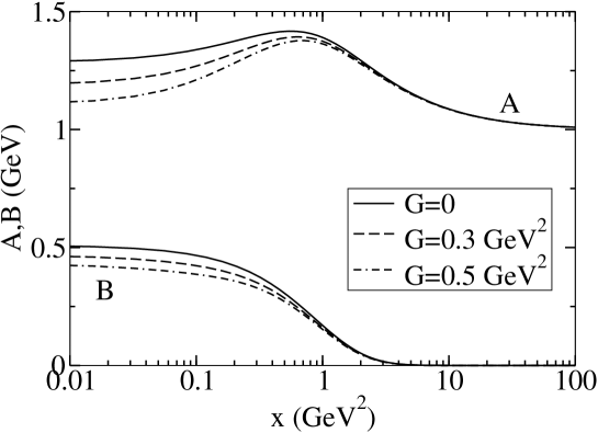
Figure 3: Spacelike quark propagator functions $A(x)$ (top curves) and $B(x)$ (lower curves) in the chiral limit, $m=0$. The rainbow truncation (solid line) is compared to the 1-loop dressed vertex model with two representative strength parameters.

The effect of vertex dressing on the quark propagator can be cast in a more physical context by considering the chiral vacuum quark condensate $\langle\overline{q}q\rangle^{0}$ which characterizes dynamical chiral symmetry breaking. In general the condensate at renormalization scale $\mu$ is

$$\langle\overline{q}q\rangle^{0}=-\lim_{\Lambda\to\infty}Z_{4}(\mu^{2},\Lambda^{2})\,N_{c}\,Tr_{D}\int^{\Lambda}\,\,\,\raisebox{-1.72218pt}{\large$\bar{}$}\!\!d\,{k}\,S_{0}(k)~{}~{}~{},$$ (22)

where $S_{0}(k)$ is the chiral limit propagator. For an extensive discussion of the condensate in QCD, see Ref. Langfeld:2003ye . The present simple model is ultraviolet convergent, regularization is not required, and $Z_{4}=1$. Eq. (22) then yields

$$\langle\overline{q}q\rangle^{0}=-\frac{3}{4\pi^{2}}\int_{0}^{\infty}dy\,y\frac{B_{0}(y)}{yA_{0}(y)^{2}+B_{0}(y)^{2}}~{}~{}~{},$$ (23)

which can be considered to be at the typical hadronic scale $\mu\sim 1~{}{\rm GeV}$. The results for $\langle\overline{q}q\rangle^{0}$ given in Table 1 show a decrease of 2% as the rainbow truncation ($G=0.0~{}{\rm GeV}^{2}$) is extended by the range of vertex dressing considered here.

Since the 2-loop BSE kernel used here preserves the axial-vector Ward-Takahashi identity, the resulting mass relation Maris:1998hd for pseudoscalar mesons is also preserved. At low $m_{q}$ this relation becomes the GMOR relation

$$(\hat{f}_{\pi}^{0})^{2}\,m_{\pi}^{2}=-2\,m_{q}\langle\overline{q}q\rangle^{0}+O(m_{q}^{2})~{}~{}~{},$$ (24)

where $\hat{f}^{0}_{\pi}=f^{0}_{\pi}/\sqrt{2}$, and $f^{0}_{\pi}$ is the chiral limit leptonic decay constant in the convention where $f_{\pi}^{\rm expt}=0.131$ GeV at the physical $u/d$-quark mass. From previous explorations Bender:1996bb ; Bender:2002as , we expect $m_{\pi}$ to be quite stable to vertex dressing; the relative insensitivity of $\langle\overline{q}q\rangle^{0}$ should therefore be evident in $f^{0}_{\pi}$ also. Here we estimate $f^{0}_{\pi}$ by using the dominant term $i\gamma_{5}\,B_{0}(q^{2})/f^{0}_{\pi}$ of the chiral pion Bethe–Salpeter amplitude Roberts:1996hh

$$(f^{0}_{\pi})^{2} = 24\int\,\,\,\raisebox{-1.72218pt}{\large$\bar{}$}\!\!d\,{q}\,B_{0}(q^{2})\left[\frac{q^{2}}{2}(\sigma^{\prime}_{v}\sigma_{s}-\sigma_{v}\sigma^{\prime}_{s})+\sigma_{v}\sigma_{s}\right]$$ (25)

$$= \frac{3}{2\pi^{2}}\int_{0}^{\infty}dy\,yB_{0}(y)\left[\frac{y}{2}\left(\sigma^{\prime}_{v}\sigma_{s}-\sigma_{v}\sigma^{\prime}_{s}\right)+\sigma_{v}\sigma_{s}\right]~{}~{}~{}.$$

This expression is known to provide an underestimate by about 10%.

The results for $f^{0}_{\pi}$ are also given in Table 1. The variation between the 1-loop (rainbow) kernel ($G=0.0~{}{\rm GeV}^{2}$) and the estimate for the physical 2-loop kernel ($G=0.5~{}{\rm GeV}^{2}$) is 1%. The expected stability of $m_{\pi}$ is confirmed from the BSE solution in Sec. V.

Table 1: The chiral quark condensate $\langle\overline{q}q\rangle^{0}$ and the chiral leptonic decay constant $f^{0}_{\pi}$ for a range of vertex dressing strength $G$ (in GeV²).

$G$	0.0	0.1	0.2	0.3	0.4	0.5	Expt
$(-\langle\overline{q}q\rangle^{0})^{1/3}$	0.2511	0.2505	0.2498	0.2492	0.2485	0.2478	0.22-0.24 GeV
$f^{0}_{\pi}$	0.1190	0.1188	0.1185	0.1183	0.1180	0.1178	0.131 GeV

To facilitate our investigation of the BSE with the 2-loop kernel, the continuation to $P^{2}=-M^{2}$ for total meson momentum will be implemented under the real axis approximation Jarecke:2002xd , defined as the substitution $F(x)\rightarrow F(\Re{x})$ where $F(x)$ stands for the quark propagator amplitudes $A(x)$ and $B(x)$ as they appear in the BSE kernel. The otherwise necessary, model-exact, method requires knowledge of the complex momentum plane structure of the BSE and DSE kernels, and has been developed and tested Maris:1999nt only for ladder truncation. Since the present 2-loop kernel is exploratory and future developments are expected, we use the approximate method here. With a ladder kernel of the present type, the real axis approximation produces values for $m_{\rho}$, $m_{K^{\star}}$ and $m_{\phi}$ that are within 4%, 7% and 1% respectively Jarecke:2002xd of the model-exact values; an accuracy of about 10% is anticipated for masses up to about 2 GeV Jarecke:2002xd .

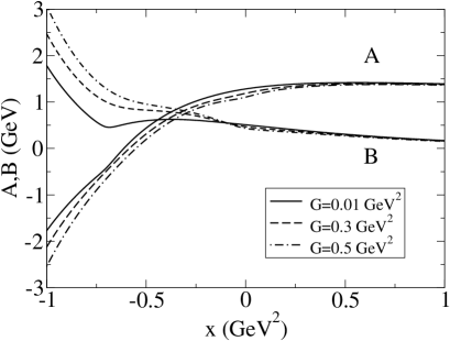
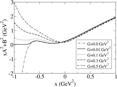
Figure 4: The influence of vertex dressing ($G>0$) on the chiral limit quark propagator for timelike and spacelike real $x=p^{2}$. Left Panel: Propagator amplitudes $A(x)$ and $B(x)$. The solid line is a good representation of the rainbow truncation. Right Panel: The denominator function. Finite vertex dressing strength prevents a zero (a physical mass-shell) in this timelike region.

Propagator amplitudes $A$ and $B$, in the chiral limit, and along the real timelike $p^{2}$ axis are displayed in Fig. 4 for representative values of the vertex dressing strength $G$. For equal mass quarks, the meson mass $M$ and the quark $x=p^{2}$ required by the BSE kernel along the real axis are related by $x>-M^{2}/4$. Thus the timelike range shown in Fig. 4 is sufficient for a meson mass up to 2 GeV. The repulsive effect of our model vertex dressing is evident in the enhanced dynamical chiral symmetry breaking ($B>0$) in the timelike region. In models of this type, the strong dynamical chiral symmetry breaking creates a significant infrared timelike domain where the dressed quark has no real mass shell; $\bar{q}q$ bound states with masses within this domain have no spurious $\bar{q}q$ decay mode. We illustrate this in Fig. 4 which displays the propagator denominator $xA(x)^{2}+B(x)^{2}$ in the chiral limit. A zero of this quantity indicates a quark mass shell. In rainbow truncation ($G=0.0$), the physical domain of applicability identified this way is $x>-0.7~{}{\rm GeV}^{2}$ Alkofer:2002bp , which allows meson states below about 1.7 GeV to be free of spurious $\bar{q}q$ widths. In Fig. 4 our model vertex dressing can be seen to enlarge the physical domain of applicability; any meson states up to 2 GeV would be without such spurious widths. This is consistent with the effective increase in infrared strength that is generated by vertex dressing.

V The Bethe–Salpeter Equation and Mesons

With the constructed 2-loop kernel, Eq. (16), the homogeneous Bethe–Salpeter equation for mesons becomes

$$\Gamma(p;P)=\int\,\,\,\raisebox{-1.72218pt}{\large$\bar{}$}\!\!d\,{k}\,K(p,k;P)_{\alpha\beta;\delta\gamma}\chi(k;P)_{\gamma\delta}$$

$$= -\frac{4}{3}\int\,\,\,\raisebox{-1.72218pt}{\large$\bar{}$}\!\!d\,{k}\,\Delta_{\mu\nu}(p-k)\gamma_{\mu}\chi(k;P)\gamma_{\nu}$$

$$-\frac{G}{12}\int\,\,\,\raisebox{-1.72218pt}{\large$\bar{}$}\!\!d\,{k}\,\Delta_{\mu\nu}(p-k)\left\{\gamma_{\mu}\chi(k;P)\gamma_{\rho}S(k_{-})\gamma_{\nu}S(p_{-})\gamma_{\rho}+\gamma_{\rho}S(p_{+})\gamma_{\mu}S(k_{+})\gamma_{\rho}\chi(k;P)\gamma_{\nu}\right\}$$

$$-\frac{G}{12}\int\,\,\,\raisebox{-1.72218pt}{\large$\bar{}$}\!\!d\,{k}\,\Delta_{\mu\nu}(p-k)\left\{\gamma_{\mu}S(k_{+})\gamma_{\rho}\chi(k;P)\gamma_{\nu}S(p_{-})\gamma_{\rho}+\gamma_{\rho}S(p_{+})\gamma_{\mu}\chi(k;P)\gamma_{\rho}S(k_{-})\gamma_{\nu}\right\}$$

$$-\frac{G}{12}\int\,\,\,\raisebox{-1.72218pt}{\large$\bar{}$}\!\!d\,{k}\,\Delta_{\mu\nu}(p-k)\left\{\gamma_{\rho}\chi(p;P)\gamma_{\mu}S(k_{-})\gamma_{\rho}S(k_{-})\gamma_{\nu}+\gamma_{\mu}S(k_{+})\gamma_{\rho}S(k_{+})\gamma_{\nu}\chi(p;P)\gamma_{\rho}\right\}$$

where the integrations over the $\delta$-functions have been carried out and $\chi(p;P)=S(p_{+})\Gamma(p;P)S(p_{-})$. Discrete solutions for meson mass $M_{n}$ exist for $P^{2}=-M_{n}^{2}$.

To solve for a particular meson, one must specify the appropriate quantum numbers $J^{PC}$ by expressing the bound state vertex $\Gamma$ in the general covariant form that has the corresponding transformation properties. The quark flavor content can be specified by the current quark masses. Here we consider pseudoscalar, vector and axial-vector charge eigenstates and adopt isospin symmetry through degenerate $u$ and $d$ quarks. The general covariant forms used here are

$$\Gamma^{PS}(p;P) = \gamma_{5}\left[\Gamma_{0}(p;P)-\imath\hbox to0.0pt{\hbox to7.80904pt{\hfil/\hfil}\hss}P\Gamma_{1}(p;P)-\imath\hbox to0.0pt{\hbox to5.03125pt{\hfil/\hfil}\hss}p\Gamma_{2}(p;P)-\left[\hbox to0.0pt{\hbox to7.80904pt{\hfil/\hfil}\hss}P,\hbox to0.0pt{\hbox to5.03125pt{\hfil/\hfil}\hss}p\right]\Gamma_{3}(p;P)\right]~{}~{},$$ (27)

$$\Gamma_{\mu}^{V}(p;P) = \gamma_{\mu}^{T}\left[\imath\Gamma_{0}(p;P)+\hbox to0.0pt{\hbox to7.80904pt{\hfil/\hfil}\hss}P\Gamma_{1}(p;P)-\hbox to0.0pt{\hbox to5.03125pt{\hfil/\hfil}\hss}p\Gamma_{2}(p;P)+\imath\left[\hbox to0.0pt{\hbox to7.80904pt{\hfil/\hfil}\hss}P,\hbox to0.0pt{\hbox to5.03125pt{\hfil/\hfil}\hss}p\right]\Gamma_{3}(p;P)\right]$$ (28)

$$+p_{\mu}^{T}\left[\Gamma_{2}(p;P)+2\imath\hbox to0.0pt{\hbox to7.80904pt{\hfil/\hfil}\hss}P\Gamma_{3}(p;P)\right]$$

$$+p_{\mu}^{T}\left[\Gamma_{4}(p;P)+\imath\hbox to0.0pt{\hbox to7.80904pt{\hfil/\hfil}\hss}P\Gamma_{5}(p;P)-\imath\hbox to0.0pt{\hbox to5.03125pt{\hfil/\hfil}\hss}p\Gamma_{6}(p;P)+\left[\hbox to0.0pt{\hbox to7.80904pt{\hfil/\hfil}\hss}P,\hbox to0.0pt{\hbox to5.03125pt{\hfil/\hfil}\hss}p\right]\Gamma_{7}(p;P)\right]~{}~{},$$

$$\Gamma_{\mu}^{AV}(p;P) = \gamma_{5}\gamma_{\mu}^{T}\left[\imath\Gamma_{0}(p;P)+\hbox to0.0pt{\hbox to7.80904pt{\hfil/\hfil}\hss}P\Gamma_{1}(p;P)-\hbox to0.0pt{\hbox to5.03125pt{\hfil/\hfil}\hss}p\Gamma_{2}(p;P)+\imath\left[\hbox to0.0pt{\hbox to7.80904pt{\hfil/\hfil}\hss}P,\hbox to0.0pt{\hbox to5.03125pt{\hfil/\hfil}\hss}p\right]\Gamma_{3}(p;P)\right]$$ (29)

$$+\gamma_{5}p_{\mu}^{T}\left[\Gamma_{2}(p;P)+2\imath\hbox to0.0pt{\hbox to7.80904pt{\hfil/\hfil}\hss}P\Gamma_{3}(p;P)\right]$$

$$+\gamma_{5}p_{\mu}^{T}\left[\Gamma_{4}(p;P)+\imath\hbox to0.0pt{\hbox to7.80904pt{\hfil/\hfil}\hss}P\Gamma_{5}(p;P)-\imath\hbox to0.0pt{\hbox to5.03125pt{\hfil/\hfil}\hss}p\Gamma_{6}(p;P)+\left[\hbox to0.0pt{\hbox to7.80904pt{\hfil/\hfil}\hss}P,\hbox to0.0pt{\hbox to5.03125pt{\hfil/\hfil}\hss}p\right]\Gamma_{7}(p;P)\right]~{}~{},$$

where the notation $a_{\mu}^{T}$ denotes a 4-vector transverse to $P_{\mu}$, i.e., $a_{\mu}^{T}=$ $t_{\mu\nu}(P)a_{\nu}$. The vector and axial-vector amplitudes $\Gamma_{\mu}^{V/AV}$ are transverse to the total momentum $P$. The $\Gamma_{i}$ are scalar functions of $p^{2}$, $p\!\cdot\!P$. For charge eigenstates, the $\Gamma_{i}$ are either odd or even under the interchange $p\!\cdot\!P\rightarrow-p\!\cdot\!P$.

For numerical solution of Eq. (LABEL:eq:bse1) we project onto the basis of Dirac covariants to obtain coupled equations for the amplitudes $\Gamma_{i}$. The dimensionality of integration is reduced by expansion of $\Gamma_{i}$ in the complete orthonormal set of Chebyshev polynomials $T_{k}(z)$ in the variable $z=p\!\cdot\!P/\sqrt{p^{2}P^{2}}$,

$$\Gamma_{i}(p^{2},z;P^{2})=\sum_{k=0}^{N_{ch}}\,i^{k}\,T_{k}(z)\,\Gamma_{i}^{k}(p^{2};P^{2})~{}~{}~{}.$$ (30)

Projection of the equation onto the $T_{k}$ basis then produces a set of coupled 1-dimensional integral equations for the $\Gamma_{i}^{k}(p^{2};P^{2})$. An explicit factor of $p\!\cdot\!P$ is extracted from the odd $\Gamma_{i}$ and an even order Chebyshev expansion is used for the remaining factor. Convergence and stability is normally achieved with $N_{ch}=4$ or $6$. The meson mass $M_{n}$ is determined by introducing a linear eigenvalue $\lambda(M)$ so that the Bethe–Salpeter equation reads

$$\lambda(M)\Gamma(p;P)_{\alpha\beta}=\int\,\,\,\raisebox{-1.72218pt}{\large$\bar{}$}\!\!d\,{k}\,\,K_{\alpha\beta;\delta\gamma}(p,k;P)\,\left[S(k_{-})\Gamma(k;P)S(k_{+})\right]_{\gamma\delta}~{}~{}~{},$$ (31)

with $P^{2}=-M^{2}$; the mass $M$ is varied until $\lambda(M=M_{n})=1$. The physical ground state in a given channel is determined by the largest real eigenvalue.

VI Numerical Results and Discussion

We explore ground state $u/d$-quark mesons and adopt the ladder kernel model of LABEL:Alkofer:2002bp which provides the parameters $\omega=0.5~{}{\rm GeV},D=16~{}{\rm GeV}^{-2}$ (see Eq. (5)) and $m_{u/d}=5$ MeV. The strength parameter $G$ for vertex dressing is varied in the range 0.0-0.5 GeV². Our model Bethe–Salpeter kernel produces real ground state masses since it does not contain a mechanism for a hadronic decay width; it also does not distinguish between isoscalar and isovector states. We indicate the physical state identifications with these qualifications in mind. Real mass solutions of the type obtained here have in the past provided a basis for successful perturbative descriptions of strong decay widths in non-scalar channels, an example being the $\rho\rightarrow\pi\pi$ width Praschifka:1987pt ; Hollenberg:1992nj ; Mitchell:1997dn .

Table 2: The $0^{-+}$ ($\pi$) and $1^{--}$ ($\rho$) masses in GeV.

$G$ (GeV2)		0	0.1	0.2	0.3	0.4	0.5	Expt
$N_{\rm ch}=$ 2	$m_{\pi}$	0.143	0.142	0.142	0.141	0.141	0.140
	$m_{\rho}$	0.806	0.808	0.810	0.811	0.812	0.813
$N_{\rm ch}=$ 4	$m_{\pi}$	0.140	0.140	0.140	0.140	0.140	0.139
	$m_{\rho}$	0.794	0.791	0.788	0.783	0.777	0.771
$N_{\rm ch}=$ 6	$m_{\pi}$	0.140	0.140	0.140	0.140	0.141	0.139	0.139
	$m_{\rho}$	0.794	0.790	0.785	0.779	0.772	0.763	0.770

Table 2 records the pion ($0^{-+}$) mass values for vertex dressing strengths between $G=0.0~{}{\rm GeV}^{2}$ (rainbow-ladder truncation) and $G=0.5~{}{\rm GeV}^{2}$ (our estimate of the physical value). The mass is practically insensitive to model details; this illustration of chiral symmetry preservation through the axial-vector Ward-Takahashi identity has been observed in related earlier work with a simplified ladder kernel Bender:1996bb ; Bender:2002as ; Bhagwat:2004hn . Table 2 also illustrates the stability and convergence with respect to $N_{\rm ch}$ (the number of Chebyschev polynomials used to expand the angle dependence of the Bethe–Salpeter amplitudes according to Eq. (30)). This and other numerical techniques were applied until an accuracy of better than 5% was achieved for the masses.

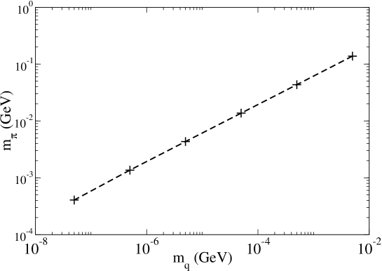
Figure 5: The $m_{q}$ dependence of the pion mass near the chiral limit. The fitted dashed line confirms that the dressed vertex model (characterized by $G=0.5~{}{\rm GeV}^{2}$) satisfies the GMOR relation, Eq. (24).

With strength $G=0.5~{}{\rm GeV}^{2}$ for vertex dressing, the $m_{q}$-dependence of the pseudoscalar bound state mass near the chiral limit is displayed in Fig. 5. The form

$$m_{\pi}=a_{1}\sqrt{m_{q}}+a_{2}\,m_{q}$$ (32)

provides a good fit with $a_{1}=1.94~{}{\rm GeV}^{\frac{1}{2}}$, and $a_{2}=0.231$. The dominance of the first term (by a factor of about 10³) suggests that the GMOR mass relation, Eq. (24), has been reproduced. This is reinforced by noting that, according to Eq. (24), we should have the correspondance $a_{1}\sim 2\sqrt{|\langle\overline{q}q\rangle^{0}|}/f^{0}_{\pi}$ and with the model value of $\langle\overline{q}q\rangle^{0}$ presented in Table 1, we deduce from the fitted $a_{1}$ that $f^{0}_{\pi}=0.1272$ GeV. This chiral value is 3% lower than the experimental value $f_{\pi}=0.1307$ GeV (at the physical mass) and is consistent with previous findings Maris:1997tm . It is also consistent with the independent calculation of $f^{0}_{\pi}$ in Section IV.

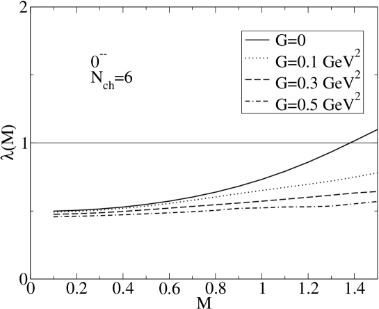
Figure 6: Exotic pseudoscalar ($0^{--}$) meson Bethe–Salpeter eigenvalue from the ladder kernel ($G=0$) and from the dressed vertex model ($G>0$).

Fig. 6 displays the eigenvalue for the exotic $0^{--}$ channel where the ladder kernel produces a mass of 1.38 GeV. Our model vertex dressing has a large repulsive effect; the physical value for $G=0.5$ GeV suggests that any mass solution would be above 2 GeV. There is a scalar $0^{++}$ solution to the present model at a mass of 0.7 GeV in ladder approximation; this decreases to 0.6 GeV for the physical 2-loop kernel. The ladder value is consistent with previous models of this type Maris:2000ig ; Burden:2002ps ; Alkofer:2002bp . A physical identification for the $0^{++}$ solution here is not appropriate because hadronic configurations such as $\bar{K}K$ are expected to play an important role, and the ladder-rainbow truncation is known to be deficient in this channel Bender:1996bb .

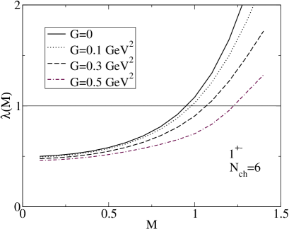
Figure 7: Axialvector meson Bethe–Salpeter eigenvalue from the ladder kernel ($G=0$) and from the dressed vertex model ($G>0$). Left Panel: The $1^{++}$ ($a_{1}/f_{1}$) state. Right Panel: The $1^{+-}$ ($b_{1}/h_{1}$) state.

The mass values for the $1^{--}$ ($\rho/\omega$) channel are presented in Table 2 for the relevant range of parameters $G$ and $N_{ch}$. The effect of the present model of 1-loop vertex dressing is seen to be an attraction of only 30 MeV. In contrast, a repulsive change of about 70 MeV applies when the delta function representation is employed for all aspects of the 2-loop kernel Bender:2002as . That simplification also provided an extension to the complete ladder summation of the one-gluon exchange mechanism for the vertex; the result being just a 75 MeV repulsion Bender:2002as . Evidently, finite momentum range effects in the kernel can influence the net result from vertex dressing and whether there is net attraction or repulsion.

However, the larger issue in the present context is why the typical effect beyond rainbow-ladder seems to be no more than $\pm$10% for the ground state vector mass when there is no explicit protection from an underlying symmetry. With the pseudoscalar state fixed by chiral symmetry, the hyperfine splitting that can be generated by modeling the quark-gluon vertex by effective gluon exchange is evidently a weak perturbation on the ladder kernel. Recent work indicates that significant attraction is provided to the dressed gluon-quark vertex by the triple-gluon vertex, and a schematic model implementation suggests that up to a 30% attractive effect on $m_{\rho}$ can be provided in this way beyond rainbow-ladder Bhagwat:2004hn . Further work is required for an understanding of how best to model the quark-gluon vertex for hadron physics.

No mass solution below 2 GeV was found in the exotic channel $1^{-+}$. In this mass range, the largest eigenvalue had reached  0.5-0.8. Masses above 2 GeV might be possible in a model of this type.

Table 3: The $1^{++}$ ($a_{1}/f_{1}$) and $1^{+-}$ ($b_{1}/h_{1}$) masses in GeV.

$G$ (GeV2)		0	0.1	0.2	0.3	0.4	0.5	Expt
$N_{\rm ch}=$ 2	$m_{a_{1}}$	1.061	1.062	1.060	1.056	1.050	1.043
	$m_{b_{1}}$	0.968	0.983	0.999	1.017	1.038	1.064
$N_{\rm ch}=$ 4	$m_{a_{1}}$	0.989	0.985	0.980	0.975	0.969	0.964
	$m_{b_{1}}$	0.952	0.978	1.008	1.046	1.094	1.155
$N_{\rm ch}=$ 6	$m_{a_{1}}$	0.989	0.982	0.975	0.969	0.963	0.959	1.230
	$m_{b_{1}}$	0.954	0.983	1.020	1.070	1.138	1.227
$N_{\rm ch}=$ 8	$m_{b_{1}}$	0.954	0.984	1.024	1.080	1.161	1.243	1.230

The eigenvalue behavior for the axial vector solutions in the $1^{++}$ ($a_{1}/f_{1}$) and $1^{+-}$ ($b_{1}/h_{1}$) channels are displayed in Fig. 7 and also in Table 3. In previous work, the ladder truncation, constrained by chiral data, is generally found to be 200-400 MeV too attractive for these P-wave states MarisPrivCom ; Jarecke:2002xd ; Alkofer:2002bp . Our present results agree with this. The $1^{++}$ channel shows a 30 MeV of attraction due to the effect of 1-loop dressing added to the ladder kernel. However, in the $1^{+-}$ ($b_{1}/h_{1}$) channel, we find a repulsive effect of 290 MeV above the ladder kernel result, yielding a value close to $m^{\rm expt}_{{\rm b}_{1}}$. We are not able to compare these findings with previous work on vertex dressing since such P-wave states do not have solutions in the models considered previously for that purpose Bender:1996bb ; Bender:2002as ; Bhagwat:2004hn . Other studies of $a_{1}$ and $b_{1}$ based on the ladder-rainbow truncation have used a separable approximation where the quark propagators are the phenomenological instruments Burden:1997nh ; Bloch:1999vk ; Burden:2002ps , these studies find more acceptable masses for both states in the vicinity of 1.3 GeV.

The typical widths of the ground state axial vector mesons are about 20% of the mass and 3$\pi$ and $4\pi$ decay channels are prominent. Although widths of this magnitude have been successfully generated perturbatively for vectors Jarecke:2002xd and axial-vectors Bloch:1999vk from BSE solutions that do not have the decay channels within the kernel, it is possible that such dynamics are responsible for important contributions to the masses beyond ladder-rainbow truncation.

VII Summary

The effect of a 1-loop model of quark-gluon vertex dressing on the masses of the light quark pseudoscalar, vector and axial-vector mesons has been studied. To facilitate calculations the vertex model consists of an effective single gluon exchange represented by a momentum $\delta$-function with strength $G$. The ladder-rainbow term is represented by a finite range effective gluon exchange. The axial-vector Ward-Takahashi identity and charge conjugation properties are used to construct a consistent Bethe–Salpeter kernel from the quark self-energy. This model extends recent explorations beyond the rainbow-ladder level by allowing axial-vector meson solutions.

At spacelike momenta the vertex dressing results in only slight corrections to the quark propagator. The Bethe–Salpeter equation was solved numerically for the ground state pseudoscalar, vector and axial-vector mesons. The results show that corrections to the rainbow-ladder truncation generate very little change to pseudoscalar masses (and effectively vector masses) when they are defined consistently with chiral symmetry.

The axial-vector mesons respond to the present vertex dressing model in a way that calls for further study. The mass of the $1^{+-}$ ($b_{1}/h_{1}$) state, too small by about 300 MeV in rainbow-ladder truncation, was raised by 290 MeV by the vertex dressing thus giving a satisfactory value. However the $1^{++}$ ($a_{1}/f_{1}$) state decreased in mass by about 30 MeV, leaving it still about 300 MeV too light compared to experiment. In the exotic meson channels, $0^{--}$ and $1^{-+}$, the vertex dressing effects are repulsive; possible solutions are well above 1.5 GeV and beyond the range of the methods of the present study.

There is very little information on the non-perturbative structure of the dressed quark-gluon vertex that can be used to guide a practical phenomenology. The Ball-Chiu (Abelian) Ansatz Ball:1980ay , often-used to generate the quark self-energy, is not useful here because the only known way to define a chiral-symmetry-preserving BSE kernel requires an explicit Feynman diagram representation of the self-energy. The present model adopts a one gluon exchange vertex structure motivated by a previous study. Dynamical information on the non-perturbative structure of the triple gluon vertex, and the contribution it can make to the quark-gluon vertex, is needed to further clarify how best to model the BSE kernel beyond ladder-rainbow. The attractive influence Bhagwat:2004hn of the triple gluon vertex can have important consequences for modeling of the hadron spectrum. The high mass meson states are furthermore exptected to move significantly when including their hadronic decay channels.

Appendix A Details of the Quark Dyson–Schwinger Equation

The quark Dyson–Schwinger equation of the present 2-loop model, Eq. (8), is

$$S^{-1}(p)=\imath\hbox to0.0pt{\hbox to5.03125pt{\hfil/\hfil}\hss}p+m+\int\,\,\,\raisebox{-1.72218pt}{\large$\bar{}$}\!\!d\,{k}\,\,\Delta_{\mu\nu}(p-k)\left\{\frac{4}{3}\gamma_{\mu}S(k)\gamma_{\nu}+\frac{G}{6}\gamma_{\mu}S(k)\gamma_{\rho}S(k)\gamma_{\nu}S(p)\gamma_{\rho}\right\}~{}~{}~{}.$$ (33)

Projection of Eq. (33) onto the basis of Dirac vector and scalar matrices produces coupled non-linear equations for the propagator amplitudes $A$ and $B$ introduced in Eq. (19). With Lorentz invariants $x=p^{2}$, $y=k^{2}$, $z=k\!\cdot\!p/\sqrt{k^{2}p^{2}}$, and integration measure $\int\,\,\,\raisebox{-1.72218pt}{\large$\bar{}$}\!\!d\,{k}\,=$ $1/(2\pi)^{3}\int_{0}^{\infty}dy\,y$ $\int_{-1}^{1}dz\,\sqrt{1-z^{2}}$, the equation then takes the form, given in Eqs. (20) and (21),

$$A(x) = I_{1}(x)+\frac{A(x)\,I_{2}(x)+B(x)\,I_{3}(x)}{xA(x)^{2}+B(x)^{2}}$$ (34)

$$B(x) = J_{1}(x)+\frac{A(x)\,J_{2}(x)+B(x)\,J_{3}(x)}{xA(x)^{2}+B(x)^{2}}~{}~{}~{},$$ (35)

where the $I_{i}(x),J_{i}(x)$ are scalar integrals over non-linear combinations of $A(y)$ and $B(y)$ for spacelike $y$. Because of the gaussian form Eq. (5) for the kernel $\Delta_{\mu\nu}(p-k)$ in the present model, the results of the angular integrations required for evaluation of $I_{i}(x)$ and $J_{i}(x)$ can be expressed in closed form. To this end one needs the two confluent hypergeometric functions Abramowitz:1968bk ,

$$Z_{\mu}^{0} =\int_{-1}^{1}dt\,\exp{\{\mu(t-1)\}}\left(1-t^{2}\right)^{-\frac{1}{2}} =\pi{}_{1}F_{1}(1/2,1;-2\mu)~{}~{}~{},$$ (36)

$$Z_{\mu}^{1} =\int_{-1}^{1}dt\,\exp{\{\mu(t-1)\}}\left(1-t^{2}\right)^{\frac{1}{2}} =\frac{\pi}{2}{}_{1}F_{1}(3/2,3;-2\mu)~{}~{}~{},$$ (37)

where $\mu=2\sqrt{xy}/\omega^{2}$. These hypergeometric functions can be numerically evaluated for general complex argument $\mu$ using their series expansion ($|\mu|<1$), direct numerical integration ($1<|\mu|<17$), or asymptotic formulae ($|\mu|>17$) Abramowitz:1968bk . There are two important cases: real $\mu$ and purely imaginary $\mu$, whereupon the angular integrals reduce to modified Bessel or Bessel functions, respectively. For real $\mu$ (i.e., real $x=p^{2}>0$)

$$Z_{\mu}^{0}=\pi e^{-\mu}I_{0}(\mu)~{}~{}~{};~{}~{}~{}~{}~{}Z_{\mu}^{1}=\frac{\pi}{\mu}e^{-\mu}I_{1}(\mu)~{}~{}~{},$$ (38)

whereas for purely imaginary $\mu$ (i.e., real $x=p^{2}<0$)

$$Z_{\mu}^{0}=\pi e^{-\mu}J_{0}(\mu^{\prime})~{}~{}~{};~{}~{}~{}~{}~{}Z_{\mu}^{1}=\frac{\pi}{\mu^{\prime}}e^{-\mu}J_{1}(\mu^{\prime})~{}~{}~{},$$ (39)

where $\mu=\imath\mu^{\prime}$. The quantities $I_{i}(x),J_{i}(x)$ can then be expressed as the one-dimensional integrals

$$I_{1}(x) = 1+\frac{2D}{\pi\omega^{2}}\int_{0}^{\infty}dy\,y\exp{\left(-\frac{(\sqrt{x}-\sqrt{y})^{2}}{\omega^{2}}\right)}\sigma_{v}(y)\times$$

$$\left[Z_{\mu}^{0}\frac{1}{2}\omega^{2}\left(1+\frac{y+2\omega^{2}}{x}\right)+Z_{\mu}^{1}\left(-y\left(2+\frac{\omega^{2}}{x}\right)-\omega^{2}\left(1+2\frac{\omega^{2}}{x}\right)\right)\right]~{}~{}~{},$$

$$I_{2}(x) = G\frac{2D}{\pi\omega^{2}}\int_{0}^{\infty}dy\,y\exp{\left(-\frac{(\sqrt{x}-\sqrt{y})^{2}}{\omega^{2}}\right)}\times$$

$$\!\!\!\!\!\!\!\!\!\!\!\!\!\!\!\!\!\!\!\!\!\!\!\!\!\!\!\!\!\!\!\!\left\{\sigma_{v}^{2}(y)\left[Z_{\mu}^{0}\frac{1}{4}\left(y\omega^{2}+\omega^{4}+\frac{y\omega^{4}+4\omega^{6}}{x}\right)+Z_{\mu}^{1}\frac{1}{4}\left(-xy-6y\omega^{2}-y^{2}-2\omega^{4}-\frac{2y\omega^{4}+4\omega^{6}}{x}\right)\right]\right.$$

$$\left.+\sigma_{s}^{2}(y)\left[Z_{\mu}^{0}\left(-\frac{\omega^{4}}{8x}\right)+Z_{\mu}^{1}\frac{\omega^{4}}{4x}\right]\right\}~{}~{}~{},$$

$$I_{3}(x) = G\frac{2D}{\pi\omega^{2}}\int_{0}^{\infty}dy\,y\exp{\left(-\frac{(\sqrt{x}-\sqrt{y})^{2}}{\omega^{2}}\right)}\sigma_{v}(y)\sigma_{s}(y)\times$$

$$\left[Z_{\mu}^{0}\frac{1}{8}\omega^{2}\left(-1-\frac{y+3\omega^{2}}{x}\right)+Z_{\mu}^{1}\frac{1}{4}\left(2y+\omega^{2}+\frac{y\omega^{2}+3\omega^{4}}{x}\right)\right]~{}~{}~{},$$

$$J_{1}(x) = m+\frac{2D}{\pi\omega^{2}}\int_{0}^{\infty}dy\,y\exp{\left(-\frac{(\sqrt{x}-\sqrt{y})^{2}}{\omega^{2}}\right)}\sigma_{s}(y)\times$$

$$\left[Z_{\mu}^{0}(-\omega^{2})+Z_{\mu}^{1}(x+y+2\omega^{2})\right]~{}~{}~{},$$

$$J_{2}(x) = G\frac{2D}{\pi\omega^{2}}\int_{0}^{\infty}dy\,y\exp{\left(-\frac{(\sqrt{x}-\sqrt{y})^{2}}{\omega^{2}}\right)}\sigma_{v}(y)\sigma_{s}(y)\times$$

$$\left[Z_{\mu}^{0}\frac{1}{8}\left(-x\omega^{2}-y\omega^{2}-3\omega^{4}\right)+Z_{\mu}^{1}\frac{1}{4}\left(2xy+x\omega^{2}+y\omega^{2}+3\omega^{4}\right)\right]~{}~{}~{},$$

$$J_{3}(x) = G\frac{2D}{\pi\omega^{2}}\int_{0}^{\infty}dy\,y\exp{\left(-\frac{(\sqrt{x}-\sqrt{y})^{2}}{\omega^{2}}\right)}\times$$

$$\!\!\!\!\!\!\!\!\!\!\!\!\!\!\!\!\!\!\!\!\!\!\!\!\!\!\!\!\!\!\!\!\left\{\sigma_{v}^{2}(y)\left[Z_{\mu}^{0}\left(-\frac{\omega^{4}}{8}\right)+Z_{\mu}^{1}\frac{\omega^{4}}{4}\right]+\sigma_{s}^{2}(y)\left[Z_{\mu}^{0}\frac{\omega^{2}}{4}+Z_{\mu}^{1}\frac{1}{4}(-x-y-2\omega^{2})\right]\right\}~{}~{}~{}.$$

The equations can be solved numerically by iteration subject to the boundary conditions $A(x)\rightarrow 1$ and $B(x)\rightarrow m$ for large spacelike $x$. Alternatively, once the spacelike integrals for $I_{i}(x),J_{i}(x)$ have been obtained, one may seek to utilize the polynomial structure of the equations in the explicitly appearing amplitudes $A(x)$ and $B(x)$. For completeness, we outline the derivation of the polynomial form.

Elimination of either $A$ or $B$ from the right-hand side of Eqs. (34) and (35) produces

$$\left[xA^{2}+B^{2}\right]\left[(A-I_{1})J_{3}-(B-J_{1})I_{3}\right]-(I_{2}J_{3}-J_{2}I_{3})A = 0$$ (41)

$$\left[xA^{2}+B^{2}\right]\left[(B-J_{1})I_{2}-(A-I_{1})J_{2}\right]-(I_{2}J_{3}-J_{2}I_{3})B = 0~{}~{},$$ (42)

where we have dropped the argument $x$ from $A$ and $B$. This can also be written as

$$\frac{(I_{2}J_{3}-J_{2}I_{3})}{\left[xA^{2}+B^{2}\right]}=\frac{(A-I_{1})J_{3}-(B-J_{1})I_{3}}{A}=\frac{(B-J_{1})I_{2}-(A-I_{1})J_{2}}{B}~{}~{}.$$ (43)

The second equality can be multiplied out to give an expression for $B^{2}$:

$$B^{2}I_{3}=B\left[A(J_{3}-I_{2})+J_{1}I_{3}-I_{1}J_{3}\right]+A^{2}J_{2}+A(J_{1}I_{2}-I_{1}J_{2})~{}~{}.$$ (44)

This expression is now used to eliminate any factors $B^{2}$ in Eqs. (41) and (42), yielding

$$B\left[A(E-C)-I_{1}E\right]+A^{2}D+A(J_{1}C-I_{1}D)-I_{3}E = 0~{}~{},$$

$$B\left[A^{2}(J_{3}E+I_{2}(C-2E))+AE(2I_{1}I_{2}-2I_{1}J_{3}+I_{3}J_{1})+E(I_{1}^{2}J_{3}-I_{1}I_{3}J_{1}-I_{3}^{2})\right]$$

$$+A^{3}J_{2}(E-C)+A^{2}(C(I_{1}J_{2}-J_{1}I_{2})+E(J_{1}I_{2}-2I_{1}J_{2}))+AEI_{1}(I_{1}J_{2}-J_{1}I_{2}) = 0~{}~{},$$

where $C=xI_{3}^{2}+I_{2}^{2}$, $D=xI_{3}J_{3}+I_{2}J_{2}$ and $E=I_{2}J_{3}-J_{2}I_{3}$. These last two equations give two equivalent expressions for $B$ so by eliminating $B$ one gets a polynomial equation involving only $A$:

$$0 =A^{4} \left[CxI_{3}+DJ_{3}-E(2xI_{3}+J_{2})\right]$$ (45)

$$+A^{3} \left[-CxI_{1}I_{3}+D(-3I_{1}J_{3}+2I_{3}J_{1})+E(4xI_{1}I_{3}+3I_{1}J_{2})\right]$$

$$+A^{2} \left[C(-I_{2}I_{3}+I_{3}J_{1}^{2})+D(-4I_{1}I_{3}J_{1}+3I_{1}^{2}J_{3}-I_{3}^{2})\right.$$

$$\left.+E(-2xI_{1}^{2}I_{3}-3I_{1}^{2}J_{2}+2I_{2}I_{3}-I_{3}J_{3})\right]$$

$$+A \left[-C(I_{1}I_{3}J_{1}^{2}+I_{3}^{2}J_{1})+D(I_{1}I_{3}^{2}+2I_{1}^{2}I_{3}J_{1}-I_{1}^{3}J_{3})\right.$$

$$\left.+E(-2I_{1}I_{2}I_{3}+2I_{1}I_{3}J_{3}+I_{1}^{3}J_{2}-I_{3}^{2}J_{1})\right]$$

$$+E(I_{1}I_{3}^{2}J_{1}-I_{1}^{2}I_{3}J_{3}+I_{3}^{3})~{}~{},$$

from whose solutions one can construct $B$ using

$$B=-\frac{A^{2}D+A(J_{1}C-I_{1}D)-I_{3}E}{A(E-C)-I_{1}E}~{}~{}.$$ (46)

The fourth order polynomial Eq. (45) has in general four solutions $A_{1},\ldots,A_{4}$ at each point $x$ with an associated $B_{1},\ldots,B_{4}$. The boundary conditions of perturbative behavior in the asymptotic spacelike region ($x\rightarrow\infty$), together with the criteria of continuity specify the physical solution.

References

- (1) P. Jain, and H. J. Munczek, Phys. Rev. D48 (1993) 5403, [arXiv:hep-ph/9307221].
- (2) P. Maris, and C. D. Roberts, Int. J. Mod. Phys. E12 (2003) 297, [arXiv:nucl-th/0301049].
- (3) C. D. Roberts and S. M. Schmidt, Prog. Part. Nucl. Phys. 45 (2000) S1, [arXiv:nucl-th/0005064].
- (4) P. Maris, and P. C. Tandy, Phys. Rev. C60 (1999) 055214, [arXiv:nucl-th/9905056].
- (5) P. Maris, and P. C. Tandy, Phys. Rev. C62 (2000) 055204, [arXiv:nucl-th/0005015].
- (6) J. Volmer et al. (The Jefferson Lab F(pi) Collaboration), Phys. Rev. Lett. 86 (2001) 1713, [arXiv:nucl-ex/0010009].
- (7) D. Jarecke, P. Maris, and P. C. Tandy, Phys. Rev. C67 (2003) 035202, [arXiv:nucl-th/0208019].
- (8) P. Maris, PiN Newslett. 16 (2002) 213, [arXiv:nucl-th/0112022].
- (9) P. Maris, and P. C. Tandy, Phys. Rev. C65 (2002) 045211, [arXiv:nucl-th/0201017].
- (10) C.-R. Ji, and P. Maris, Phys. Rev. D64 (2001) 014032, [arXiv:nucl-th/0102057].
- (11) R. Alkofer, and L. von Smekal, Phys. Rept. 353 (2001) 281, [arXiv:hep-ph/0007355].
- (12) P. Maris, C. D. Roberts, and P. C. Tandy, Phys. Lett. B420 (1998) 267, [arXiv:nucl-th/9707003].
- (13) H. J. Munczek, and A. M. Nemirovsky, Phys. Rev. D28 (1983) 181.
- (14) A. Bender, C. D. Roberts, and L. v. Smekal, Phys. Lett. B380 (1996) 7, [arXiv:nucl-th/9602012].
- (15) R. Alkofer, P. Watson, and H. Weigel, Phys. Rev. D65 (2002) 094026, [arXiv:hep-ph/0202053].
- (16) P. Maris (2001), private communication.
- (17) C. J. Burden, L. Qian, C. D. Roberts, P. C. Tandy, and M. J. Thomson, Phys. Rev. C55 (1997) 2649, [arXiv:nucl-th/9605027].
- (18) C. J. Burden, and M. A. Pichowsky, Few Body Syst. 32 (2002) 119, [arXiv:hep-ph/0206161].
- (19) J. C. R. Bloch, Y. L. Kalinovsky, C. D. Roberts, and S. M. Schmidt, Phys. Rev. D60 (1999) 111502, [arXiv:nucl-th/9906038].
- (20) J. I. Skullerud, P. O. Bowman, A. Kizilersu, D. B. Leinweber, and A. G. Williams, JHEP 0304 (2003) 047, [arXiv:hep-ph/0303176].
- (21) J. S. Ball, and T.-W. Chiu, Phys. Rev. D22 (1980) 2542.
- (22) C. S. Fischer, and R. Alkofer, Phys. Rev. D67 (2003) 094020, [arXiv:hep-ph/0301094].
- (23) H. J. Munczek, Phys. Rev. D52 (1995) 4736, [arXiv:hep-th/9411239].
- (24) A. Bender, W. Detmold, C. D. Roberts, and A. W. Thomas, Phys. Rev. C65 (2002) 065203, [arXiv:nucl-th/0202082].
- (25) M. S. Bhagwat, A. Holl, A. Krassnigg, C. D. Roberts, and P. C. Tandy (2004), [arXiv:nucl-th/0403012].
- (26) P. Maris, and C. D. Roberts, Phys. Rev. C56 (1997) 3369, [arXiv:nucl-th/9708029].
- (27) J. M. Cornwall, R. Jackiw, and E. Tomboulis, Phys. Rev. D10 (1974) 2428.
- (28) K. Langfeld, H. Markum, R. Pullirsch, C. D. Roberts and S. M. Schmidt, Phys. Rev. C67 (2003) 065206, [arXiv:nucl-th/0301024].
- (29) C. D. Roberts, Nucl. Phys. A605 (1996) 475, [arXiv:hep-ph/9408233].
- (30) J. Praschifka, C. D. Roberts and R. T. Cahill, Int. J. Mod. Phys. A2 (1987) 1797.
- (31) L. C. L. Hollenberg, C. D. Roberts, and B. H. J. McKellar, Phys. Rev. C46 (1992) 2057.
- (32) K. L. Mitchell, and P. C. Tandy, Phys. Rev. C55 (1997) 1477, [arXiv:nucl-th/9607025].
- (33) P. Maris, C. D. Roberts, S. M. Schmidt, and P. C. Tandy, Phys. Rev. C63 (2001) 025202, [arXiv:nucl-th/0001064].
- (34) M. Abramowitz, and I. A. Segun, ”Handbook of Mathematical Functions”, Dover Publications (1968).