Clan structure analysis and QCD parton showers
in multiparticle dynamics.
An intriguing dialog between theory and experiment

Abstract

This paper contains a review of the main results of a search of regularities in collective variables properties in multiparticle dynamics, regularities which can be considered as manifestations of the original simplicity suggested by QCD. The method is based on a continuous dialog between experiment and theory. The paper follows the development of this research line, from its beginnings in the seventies to the current state of the art, discussing how it produced both sound interpretations of the most relevant experimental facts and intriguing perspectives for new physics signals in the TeV energy domain.

1 INTRODUCTION

The structure of the vacuum and confinement are still unsolved problems of Quantum Chromodynamics (QCD) after many years from its introduction as the theory of strong interactions. Sound experimental informations in order to approach the two problems can come from hadronic spectrum and multiparticle production data. Attention in the present work is focused on multiparticle production and concerns mainly collective variables properties of final charged particles in full phase-space and restricted rapidity intervals, i.e., of collective variables properties in those awkward sectors where perturbative QCD is hardly applicable. Guiding line is the conviction that complex structures which we observe at final hadron level might very well be, at the origin of their evolution, elementary and have simple properties. These characteristics in the detected observables are revealed by the occurrence of regularities which are expected to contain signals of the original simplicity and to be expressed in terms of the minimum number of physical parameters.

This research line, along the years, has been inspiring and quite successful for a phenomenological description, based on essentials of QCD, of the main experimental facts in multiparticle dynamics. This paper contains a summary of the results of this endeavour, which might be quite stimulating in the approach to the TeV energy domain in $pp$ and heavy ion collisions, and to the determination of their possible substructures.

Multiparticle production has quite a long story and its understanding is indeed crucial for strong interaction. The first observation of such events goes back to cosmic ray physics in the thirties of the past century: the extraordinary and impressive fact had been the non-linearity of the phenomenon.

This unusual experimental observation attracted the attention of many theorists in the forties and early fifties: in particular, the work of E. Fermi on the thermodynamical model [1] and of L. Landau [2] on the hydrodynamical model should be mentioned. Of course the contributions by J.F. Carlson and J.R. Oppenheimer [3], H.J. Bhabha and W. Heitler [4], W.H. Furry [5], H.W. Lewis, J.R. Oppenheimer, S.A. Wouthuysen [6], together with the pioneering work by N. Arley [7] should not be forgotten. Particular aspects of the new experimental fact were described, but the situation was considered not satisfactory from a theoretical point of view. It was only W. Heisenberg who understood that multiparticle production should be described in terms of a non-linear field theory of a new nuclear force (which we call today indeed strong interaction) [8].

With the incoming of the multi-peripheral model [9], an important step was done in the understanding of the c.m.  energy dependence of the average charged particle multiplicity in high energy collisions in terms of a logarithmic function, a trend competitive with the square root rule proposed earlier on purely phenomenological grounds [10]; $n$ charged particle multiplicity distribution (MD), $P_{n}$, was predicted to be Poissonian, when plotted vs. $n$, suggesting an independent particle production process. Few years later (in 1966), P.K. MacKeown and A.W. Wolfendale noticed, in cosmic ray experiments, remarkable violations in the dynamical mechanism for independent particle production, by observing quite large fluctuations of the pionization component in hadron showers originated by primary hadrons at different primary energies [11]. They proposed to fit high energy cosmic ray data on charged particle multiplicity distributions (MD’s) in terms of a Negative Binomial (Pascal) multiplicity distribution [from now on abbreviated as NB(Pascal)MD]. This phenomenological distribution is in fact characterised by an extra parameter in addition to the average charged multiplicity $\bar{n}$, i.e., the parameter $k$ which is linked to the dispersion $D$: $k=\bar{n}^{2}/(D^{2}-\bar{n})$. $D^{2}>\bar{n}$ implies indeed deviations from the Poissonian behaviour of the $n$-particle MD predicted by the multi-peripheral model to which the NB (Pascal) MD reduces for $k\to\infty$. The Authors gave also a sound phenomenological expression for the energy dependence of $k^{-1}$, showing that it is a finite number which increases with the increasing of the energy of the primary hadron toward an asymptotic constant value ($k^{-1}\approx 0.4$).

The discovery in the accelerator region, in the seventies, of the violations of multi-peripheral model predictions on $n$ charged particle multiplicity distribution in high energy hadron-hadron collisions [12] confirmed the cosmic ray physics findings. The parallel success of the NB (Pascal) MD in describing in full phase-space in the accelerator region $n$ charged particle multiplicity distributions at different $p_{\text{lab}}$ in various collisions (53 experiments were successfully fitted [13, 14] led to guess that the distribution was a good candidate for representing multi-peripheral model prediction violations. Although a germane attempt to justify the occurrence of the distribution in terms of the so called generalised multi-peripheral bootstrap model [15] was quickly forgotten, its phenomenological interest remained in the field: the distribution was rediscovered in full phase-space for non-single diffractive events and extended to (pseudo)-rapidity intervals by UA5 Collaboration [16] at CERN $p\bar{p}$ Collider c.m. energies, and then successfully used by NA 22 Collaboration [17] at $\sqrt{s}=22$ GeV in $pp$ and $\pi^{\pm}p$ collisions and by HRS experiment [18] in $e^{+}e^{-}$ annihilation at $\sqrt{s}=29$ GeV in order to describe $P_{n}$ vs. $n$ behaviour both in full phase-space and in symmetric (pseudo)rapidity intervals.

The last two experiments were of great importance: the first one established a low energy point in hadron-hadron collisions, the second one extended to a new class of collisions the interest for the NB (Pascal) MD. In comparing NA22 with UA5 data it was found that $\bar{n}$ increases and $k$ parameter decreases in full phase-space as the c.m. energy becomes larger, whereas at fixed c.m. energy $\bar{n}$ and $k$ become larger with the increase of (pseudo)rapidity interval. ISR, TASSO and EMC collaborations data on $P_{n}$ vs. $n$ followed within a short time and confirmed the success of their description by means of NB (Pascal) MD [19, 20, 21]. The fact that so many experiments in a so wide energy range and in symmetric (pseudo)-rapidity interval could be fitted by the same $n$ charged particle MD was considered not accidental. The impression was that one was facing an approximate universal regularity.

A suggestive interpretation of the regularity was then proposed: it implied that the dynamical mechanism controlling multiparticle production in high energy collisions is a two-step process. To the independent (Poissonian) production of groups of ancestor particles (called “clan ancestors”) follows their decay according to a (logarithmic) hadron shower process (the particle MD within each clan). Clans are by definition independently produced and, by assumption, exhaust all existing particle correlations within each clan (the “clan” concept was introduced in high energy physics at the XVII International Symposium on Multiparticle Dynamics [22]). This interpretation gave a sound qualitative description of different classes of collisions in terms of the two new parameters, the average number of clans, $\bar{N}$, and the average number of particles per clan, ${\bar{n}_{c}}$, two non-trivial functions of standard NB (Pascal) MD parameters $\bar{n}$ and $k$ (the study of $\bar{N}$ and ${\bar{n}_{c}}$ constitutes what is known as clan structure analysis, described in more detail in Section 2.2).

It turned out that within this analysis the average number of clans was larger in $e^{+}e^{-}$  annihilation than in $pp$ collisions, but the average number of particles per clan was smaller in $e^{+}e^{-}$  annihilation than in $pp$. The situation was intermediate between the last two in deep inelastic scattering (the average number of clans was smaller than in $e^{+}e^{-}$  annihilation and similar to the average number in $pp$ collisions, but the average number of particle per clan was more numerous than in $e^{+}e^{-}$  annihilation.) Larger clans in $p\bar{p}$ collisions with respect to those in $e^{+}e^{-}$  annihilation were interpreted as an indication of a stronger colour exchange mechanism in the initial state of the collision in hadron-hadron collisions with respect to $e^{+}e^{-}$  annihilation. The advent of QCD as the theory of of strong interactions —the non-linear field theory foreseen by W. Heisenberg— raised a new question, i.e., how to reconcile observed final $n$ charged particle MD’s in various collisions, all described by NB (Pascal) MD’s, with QCD expectations for final parton MD’s.

The problem was considered quite challenging and intriguing in view of the fact that, in solving QCD Konishi-Ukawa-Veneziano (KUV) parton differential evolution equations in the leading-log approximation with a fixed cut-off regularization prescription, jets initiated by a quark and a gluon were found to be QCD Markov branching processes controlled by quark bremsstrahlung and gluon self-interaction QCD vertices, and final parton multiplicity distributions were in both cases found to be again NB (Pascal) MD’s [23, 24]. In order to solve the puzzle, in consideration of the lack of explicit QCD calculations at final parton level, the suggestion was to rely on Monte Carlo calculations based on Dokshitzer-Gribov-Lipatov-Altarelli-Parisi (DGLAP) integral QCD evolution equations (the integral version of the KUV differential QCD evolution equations) and on a convenient guesswork as hadronization prescription. It was found [25, 26], by using the Jetset 7.2 Monte Carlo, that NB (Pascal) MD occurred both at final hadron and parton level multiplicity distributions for $q\bar{q}$ and $gg$ systems at various c.m. energies and in symmetric rapidity intervals. Results at parton and hadron levels turned out not to be independent and their relation summarised in the so called ‘generalised’ local hadron(h) - parton(p) duality (GLPHD), i.e., $k_{h}=k_{p}$ and $\bar{n}_{h}=\rho\bar{n}_{p}$. The name ‘generalised’ came from the need to distinguish the present ‘strong’ result from the standard ‘weak’ local hadron parton duality (LPHD) which requested in its first version that only the second of the two equations be satisfied. Others unexpected regularities emerged when Monte Carlo results were analysed in terms of clan structure analysis [25, 26].

Apparently the situation was quite well settled, but as it very often happens in the continuous dialog between theory and experiment (the main characteristic of the field), new experimental facts were just around the corner ready to question the universality of the regularity, i.e., the statement that final $n$ charged particle multiplicity distributions in all classes of collisions both in full phase-space (FPS) and in symmetric (pseudo)-rapidity intervals are NB (Pascal) MD’s. Experiments at top CERN $p\bar{p}$ Collider energy (UA5 Collaboration, [27]) and in $e^{+}e^{-}$  annihilation at LEP energies (Delphi Collaboration [28, 29]) showed a shoulder structure in $P_{n}$ vs. $n$ plots for the total sample of events both in FPS and in larger (pseudo)-rapidity intervals. In conclusion, the regularity was violated as the c.m. energy of the collision increased. Since the regularity, in view also of the quite large experimental errors, has been always considered to be true in an approximate sense, a better analysis of the existing data, together with the new data on the shoulder structure of $P_{n}$ vs. $n$ plot, led to guess that these new facts were signals of substructures arising as the c.m. energy increased.

Then an amusing situation happened: the regularities in terms of NB (Pascal) MD could be restored at a more fundamental level of investigation, i.e., at the level of the different classes of events contributing to the total sample (for instance the classes of soft and semi-hard events in $p\bar{p}$ collisions and the classes of the two- and the three-jet sample of events in $e^{+}e^{-}$ annihilation) [30, 31, 32].

The result was that the weighted superposition mechanism of different classes of events (each one described by a NB (Pascal) MD with characteristic parameters $\bar{n}$ and $k$) in different collisions allowed to describe quite successfully, in addition to the shoulder effect in $P_{n}$ vs. $n$, also the observed $H_{n}$ vs. $n$ oscillations (where $H_{n}$ is the ratio of $n$-factorial cumulants, $K_{n}$, to $n$-factorial moments $F_{n}$ and the truncation effect had been properly taken into account [32]) and the general behaviour of the energy dependence of the strength of forward-backward (FB) multiplicity correlations (MC’s) [33].

Finally, extrapolations of collective variables for the different classes of events based on our knowledge of the GeV energy domain became possible in the TeV region accessible at LHC. Expected data on $pp$ collisions at LHC will test these predictions.

Clan concept emerges as fundamental in this new context and its relevance in the theoretical interpretation of the above mentioned results leads to the conclusion that it would not be too bold to ask to experiment and theory respectively the following two questions:

Are clans real physical observable quantities?

What is the counterpart of clans at parton level in QCD?

In addition, in our approach, signals of new physics at LHC in restricted rapidity intervals are foreseen in the total sample of events for $P_{n}$ vs. $n$ (elbow structure) as a consequence of the reduction of the average number of clan to few units in an eventual third class of events (described by a NB (Pascal) MD with $k<1$). The new class should be added to the soft and semi-hard ones. All together, the above mentioned facts form what has been called “the enigma of multiparticle dynamics”, which we would like to disentangle in this paper.

The last word is once more to experimental observation, of course, and is challenging for QCD! The problem in multiparticle phenomenology can be summarised in fact in the following simple terms.

A rigorous application of QCD is limited to hard interactions only. They occur at very small distances and large momentum transfers among quarks and gluons (the elementary constituents of the hadrons), and in very short times. Perturbative QCD can be applied with no limitations in these regions. A situation which should be contrasted with the fact that the majority of strong interactions are soft; they occur in relatively large time interval and distances among constituents, and large transverse momenta. The search should be focused on how to build a bridge between hard and soft interactions, and between soft interactions and the hadronization mechanism, i.e., on how to explore regions not accessible to perturbative QCD, like those with high parton densities. Along this line of thought it is compulsory to isolate in these extreme regions the properties of the sub-structures or components or classes of events contributing to the total sample of events, being aware of the fact that the only informations we can rely on in a collision —as already pointed out— are coming from the hadronic spectrum and multiparticle production. The present work (limited to multiparticle dynamics) has been motivated by the need to review experimental facts and theoretical ideas in the field, ideas which, after more than thirty years from their introduction in the accelerator region, are still with us today and arouse a special interest [34, 35, 36, 37].

The experimental facts we are referring to are indeed very important in establishing collective variables behaviour in full phase-space and restricted rapidity intervals and represent the natural starting point for the investigations of the new horizon, opened at CERN and RHIC, in the TeV domain for hadron-hadron and nucleus-nucleus collisions.

On the theory side, the ideas we propose to examine are still quite stimulating and matter of debate in view of both their success in describing, with good approximation, important aspects of multiparticle phenomenology of high energy collisions and of their connection with QCD parton showers. The search started a long time ago and took advantage of the encouragement and great interest of many scientists; of particular relevance has been the contribution of Léon Van Hove who, we are sure, would be very glad to see how far some ideas elaborated together went.

In Section 2, in order to enlarge the scope of our work from a phenomenological point of view, we decided to discuss the main statistical properties of the collective variables of the class of MD’s to which NB (Pascal) MD belongs, i.e., the class of Compound Poisson Multiplicity Distributions (CPMD). Within this framework particular attention is paid to clan concept and its generalisations in view of its relevance in our approach to multiparticle phenomenology. Clan structure properties are always exemplified in the case of the NB (Pascal) MD.

In Section 3, QCD roots of NB (Pascal) MD are examined by studying jets at parton level as QCD Markov branching processes in the framework of QCD KUV equations. Then an attempt is presented to build a model of parton cascading based on essentials of QCD (gluon self-interaction) in a correct kinematical framework. This study led us to the generalised simplified parton shower model (GSPS) with two parameters.

In Section 4, global properties of collective variables in multiparticle dynamics in various experiments are discussed and their descriptions and interpretations in terms of clan structure analysis are presented. Attention is focused especially on $n$ charged particle MD’s general behaviour in FPS and in (pseudo)-rapidity intervals in $pp$ collisions and $e^{+}e^{-}$ annihilation, on the oscillation of the ratio of $n$-order factorial cumulants to factorial moments when plotted vs. $n$ and on forward-backward multiplicity correlations. This study is extended in $pp$ collisions to different scenarios in the TeV energy domain and has been obtained by extrapolating our knowledge of the collisions in the GeV region. It is shown that the weighted superposition mechanism of different classes of events, each one described by a NB (Pascal) MD provides a satisfactory description of all above mentioned, more subtle aspects of multiparticle phenomenology. Clan structure analysis turns out to be quite important in this respect. Its success raises a natural question on the physical properties of clans. New perspectives opened by the reduction of the average number of clans in the semi-hard component of the scenarios with Koba-Nielsen-Olesen (KNO) scaling violation are examined. Signals of new physics in $pp$ collisions in the TeV region (ancillary to those expected for heavy ion collisions) are discussed at the end.

2 COLLECTIVE VARIABLES AND CLAN STRUCTURE ANALYSIS

In studying and testing perturbative QCD, two complementary approaches can be used: one can select infrared-safe quantities in order to test pQCD in the hard region, where calculations are well defined and non-perturbative corrections are suppressed. Alternatively, one can examine infrared-sensitive observables with the aim of testing the validity of the theory in the long-range region, where confinement becomes dominant. It could be said that the latter approach determines the boundary conditions that the former one must satisfy. The present work takes the road of the infrared-sensitive observables, which are discussed in detail in this Section [38, 39, 40].

2.1 Observables in multiparticle production. The collective variables.

In a $n$-particle production process in the collision of particles $a$ and $b$

$$a+b\to c_{1}+\dots+c_{n},$$ (1)

by assuming for simplicity that all produced particles $c_{i}$ are of the same species, the $n$-particle exclusive distribution $P_{n}^{\prime}(y_{1},\dots,y_{n})$ in a sub-domain of phase-space (the $y_{i}$ with $i=1\dots n$ are the particle (pseudo)-rapidities) is described in terms of exclusive cross sections, i.e.,

$$P_{n}^{\prime}(y_{1},\dots,y_{n})=(\sigma_{\text{inel}})^{-1}\frac{d^{n}{\sigma_{n}}}{dy_{1}\dots dy_{n}}$$ (2)

and is fully symmetric in its variables. $P_{n}^{\prime}(y_{1},\dots,y_{n})$ is related to the probability of detecting $n$ particles at rapidity variables $y_{1},\dots,y_{n}$ with no other particle present in the subdomain.

The corresponding integrated observable in the rapidity interval $\Delta y$, (i.e., one integrates over $y_{i}\in\Delta y$, $i=1,\dots,n$) describes the probability $P_{n}(\Delta y)$ of detecting $n$ particles in the mentioned interval and is the $n$-particle exclusive cross section, $\sigma_{n}$, normalised to the total inelastic cross section, $\sigma_{\text{inel}}$:

$$P_{n}(\Delta y)=\frac{\sigma_{n}}{\sigma_{\text{inel}}}=(n!)^{-1}\int_{\Delta y}\dots\int_{\Delta y}P_{n}^{\prime}(y_{1},...,y_{n})dy_{1}\cdots dy_{n}.$$ (3)

The $n$-particle inclusive distribution, $Q_{n}(y_{1},\dots,y_{n})$, in the reaction

$$a+b\to c_{1}+\dots+c_{n}+\text{anything}$$ (4)

describes the finding of $n$ particles at $y_{1},\dots,y_{n}$, without paying attention to other particles in the same sub-domain, in terms of the $n$-particle inclusive cross-section density, i.e.,

$$Q_{n}(y_{1},\dots,y_{n})=({\sigma_{\text{inel}}})^{-1}\frac{d^{n}\sigma}{dy_{1}\cdots dy_{n}}$$ (5)

(sometimes referred to in the literature as $\rho(y_{1},\dots,y_{n})$.)

The corresponding integrated observables in $\Delta y$,

$$F_{n}(\Delta y)=\int_{\Delta y}\dots\int_{\Delta y}Q_{n}(y_{1},\dots,y_{n})dy_{1}\cdots dy_{n},$$ (6)

are the un-normalised $n$-factorial moments of the multiplicity distribution in $\Delta y$ (the so-called binomial moments). For instance the average multiplicity in $\Delta y$, $\bar{n}(\Delta y)$, is

$$F_{1}(\Delta y)=\bar{n}(\Delta y)=\int_{\Delta y}Q_{1}(y_{1})dy_{1}=\int_{\Delta y}\frac{d{\sigma}}{dy_{1}}dy_{1}$$ (7)

In the integration over the domain $\Delta y$ each particle will contribute once to the $n$-particle event and the event will be counted $n$ times. Coming to the second order factorial moment, $F_{2}(\Delta y)=\langle(n-1)n\rangle$, each ordered couple of final particles will be counted once in one event and the event will be counted $2\binom{n}{2}$ times.

The $n$-particle inclusive distributions $Q_{n}(y_{1},\dots,y_{n})$ contain inessential contributions due to combinations of inclusive distributions of lower order. In addition, for large $n$, it is hard to measure all $Q_{n}(y_{1},\dots,y_{n})$ and a more essential information is demanded. Accordingly, a new set of observables is introduced, the set of $n$-particle correlation functions $C_{n}(y_{1},...,y_{n})$ which reminds of cluster-expansion in statistical mechanics:

$$\begin{split}Q_{1}(y_{1})&=C_{1}(y_{1})\\ Q_{2}(y_{1},y_{2})&=C_{2}(y_{1},y_{2})+C_{1}(y_{1})C_{1}(y_{2})\\ Q_{3}(y_{1},y_{2},y_{3})&=C_{3}(y_{1},y_{2},y_{3})+C_{1}(y_{1})C_{2}(y_{2},y_{3})+\\ &\quad~{}C_{1}(y_{2})C_{2}(y_{3},y_{1})+C_{1}(y_{3})C_{2}(y_{1},y_{2})+\\ &\quad~{}C_{1}(y_{1})C_{1}(y_{2})C_{1}(y_{3})\\ \ldots\end{split}$$ (8)

The reverse is of course always possible and one can express $C_{n}(y_{1},\dots,y_{n})$ variables in terms of $Q_{n}(y_{1},\dots,y_{n})$ variables: the $n$-particle correlation functions $C_{n}(y_{1},\dots,y_{n})$ give precious informations on the production process:

$$C_{n}(y_{1},\dots,y_{n})=0\quad\Rightarrow\quad Q_{n}(y_{1},\dots,y_{n})={\prod_{i=1}^{n}}Q_{1}(y_{i})$$ (9)

Produced particles are Poissonianly distributed.

$$C_{n}(y_{1},\dots,y_{n})>0$$ (10)

Produced particles follow a distribution wider than a Poisson distribution.

$$C_{n}(y_{1},\dots,y_{n})<0$$ (11)

Produced particles follow a distribution narrower than a Poisson distribution.

The corresponding integrated observable are called factorial cumulants of the multiplicity distribution and indicated in the literature with $K_{n}$. They give informations on the shape of the multiplicity distribution when plotted vs. $n$, i.e., on its dispersion $\langle(n-\bar{n})^{2}\rangle$, skewness $\langle(n-\bar{n})^{3}\rangle$, kurtosis $\langle(n-\bar{n})^{4}\rangle$, ….

Both $F_{n}$ and $K_{n}$ are sensitive to events with many particles and control the tail of the multiplicity distribution. In $K_{n}$ are subtracted the $Q_{n-1},...,Q_{1}$ correlations present in $Q_{n}$, not those related to the fluctuations in the multiplicity, as lucidly discussed in [41].

Usually normalised differential collective variables

$$\tilde{Q}_{n}=Q_{n}(y_{1},\dots,y_{n})/Q_{1}(y_{1})\dots Q_{1}(y_{n}),$$ (12)

$$\tilde{C}_{n}=C_{n}(y_{1},\dots,y_{n})/C_{1}(y_{1})\dots C_{1}(y_{n})$$ (13)

and the corresponding normalised integral collective variables:

$$\tilde{F}_{n}=F_{n}(\Delta y)/F_{1}(\Delta y)\dots F_{1}(\Delta y),$$ (14)

$$\tilde{K}_{n}=K_{n}(\Delta y)/K_{1}(\Delta y)\dots K_{1}(\Delta y)$$ (15)

are used.

In the literature also $n$-particle combinants $W_{n}(\Delta y)$ are defined. Their expression is a function of $n$-particle multiplicity distribution $P_{n}(\Delta y)$ according to the following recurrence relation:

$$W_{n}(\Delta y)=\frac{P_{n}(\Delta y)}{P_{0}(\Delta y)}-\frac{1}{n}{\sum_{i=1}^{n-1}}iW_{i}(\Delta y)\frac{P_{n-i}(\Delta y)}{P_{0}(\Delta y)},$$ (16)

i.e., $W_{n}$ are “finite combination” ratios of $P_{n}$ to $P_{0}$. The name combinants comes from this fact.

Combinants in their normalised form, $\tilde{W}_{n}$ are

$$\tilde{W}_{n}(\Delta y)=\frac{W_{n}(\Delta y)}{[W_{1}(\Delta y)]^{n}}.$$ (17)

Notice that combinants are linked to factorial cumulants $K_{n}$ i.e.

$$W_{n}(\Delta y)=\frac{1}{n!}{\sum_{i=0}^{\infty}}\frac{(-1)^{i}K_{i+n}(\Delta y)}{i!}.$$ (18)

Of particular interest is the relation which allows to express $P_{0}(\Delta y)$ in terms of the combinants:

$$P_{0}(\Delta y)=\exp\left[-\sum_{n=1}^{\infty}W_{n}\right].$$ (19)

From the definition and properties of combinants it turns out that they are sensitive to the head of the multiplicity distribution whereas factorial cumulants and moments are sensitive to the tail of the multiplicity distribution.

The relation among collective differential variables $P_{n}^{\prime}(y_{1},\dots,y_{n})$, $Q_{n}(y_{1},\dots,y_{n})$ and $C_{n}(y_{1},\dots,y_{n})$ can be elegantly reformulated in terms of functionals, i.e., of $G[z(y)]$ with $z(y)=1+u(y)$ and $u(y)$ an arbitrary function of $y$. Within this framework, $G[z(y)]$ is defined as follows

$$G[z(y)]=P_{0}+\sum_{n=1}^{\infty}(n!)^{-1}\int_{\Delta y_{1}}\dots\int_{\Delta y_{n}}P_{n}^{\prime}(y_{1},\dots,y_{n})\prod_{i=1}^{n}z(y_{i})dy_{i},$$ (20)

i.e., the (exclusive) generating functional. It should be noticed that

$$P_{0}=1-\sum_{n=1}^{\infty}(n!)^{-1}\int_{\Delta y_{1}}\dots\int_{\Delta y_{n}}P_{n}^{\prime}(y_{1},\dots,y_{n})dy_{1}\dots dy_{n}$$ (21)

is the probability of events with zero particle multiplicity.

The knowledge of the functional $G[z(y)]$ allows to define two other functionals $G[u(y)]$ and $g[u(z)]$. They are linked by the relation

$$G[u(y)]=\exp\left\{g[u(y)]\right\},$$ (22)

where

$$G[u(y)]=1+{\sum_{n=1}^{\infty}}(n!)^{-1}\int_{\Delta y_{1}}\dots\int_{\Delta y_{n}}Q_{n}(y_{1},\dots,y_{n})\prod_{i=1}^{n}u(y_{i})dy_{i},$$ (23)

is the (inclusive) generating functional, and

$$g[u(y)]={\sum_{n=1}^{\infty}}(n!)^{-1}\int_{\Delta y_{1}}\dots\int_{\Delta y_{n}}C_{n}(y_{1},\dots,y_{n})\prod_{i=1}^{n}u(y_{i})dy_{i}.$$ (24)

It is remarkable that, in view of the existing connection among collective differential variables $P_{n}^{\prime}$, $Q_{n}$, $C_{n}$ and their integrated partners $P_{n}$, $F_{n}$, $K_{n}$, the generating functions (GF’s) of the integrated variables, obtained by the substitution $z(y)\to z$, are $G(z)$, $G(z+1)$ and $\log G(z+1)$ respectively. Accordingly, being $G(z)=\sum_{n}P_{n}z^{n}$ it follows

$$P_{n} =\frac{1}{n!}\left.\frac{\partial^{n}G(z)}{\partial z^{n}}\right|_{z=0},$$ (25)

$$F_{n} =\left.\frac{\partial^{n}G(z)}{\partial z^{n}}\right|_{z=1},$$ (26)

$$K_{n} =\left.\frac{\partial^{n}\log G(z)}{\partial z^{n}}\right|_{z=1}.$$ (27)

In addition one gets

$$G(z)=\exp{\sum_{n=1}^{\infty}}\frac{z^{n}K_{n}}{n!}=\prod_{n=1}^{\infty}\exp\left[\frac{z^{n}K_{n}}{n!}\right].$$ (28)

Coming to multiplicity combinants $W_{n}(\Delta y)$ their relation with the exclusive generating function $G(z;\Delta y)$ should be recalled:

$$G(z;\Delta y)=\exp\left[\sum_{n=1}^{\infty}W_{n}(\Delta y)(z^{n}-1)\right].$$ (29)

This relation shows that combinants are the coefficients of the power series expansion of the logarithm of the generating function.

The above general definitions will now be exemplified for the NB (Pascal) MD; explicit expressions are given below, and also plotted in Fig. 1 for typical values of the parameters (corresponding to the soft and semi-hard components which describe $pp$  collisions data at 546 GeV c.m. energy [42].)

Being the GF of the NB (Pascal) MD

$$G_{\text{NB}}(z)=\left(\frac{k}{k-(z-1)\bar{n}}\right)^{k}$$ (30)

(with $k^{-1}=(D^{2}-\bar{n})/\bar{n}^{2}$, $D$ is the dispersion) it is found from Eq.s (25), (26), (27) that

$$P^{\text{(NB)}}_{n}=\frac{k(k+1)\cdots(k+n-1)}{n!}\frac{\bar{n}^{n}k^{k}}{(\bar{n}+k)^{k+n}},$$ (31)

$$F^{\text{(NB)}}_{n}=\bar{n}^{n}{\prod_{i=1}^{n-1}}(1+i/k),$$ (32)

and

$$K^{\text{(NB)}}_{n}=\bar{n}^{n}{\prod_{i=1}^{n-1}}i/k.$$ (33)

In the literature also the collective variables expressed in terms of the ratio of factorial cumulants and moments [43], i.e.,

$$H_{n}=K_{n}/F_{n},$$ (34)

deserve great attention. For the NB (Pascal) MD one gets

$$H^{\text{(NB)}}_{n}={\prod_{i=1}^{n-1}}\frac{i}{(i+k)}.$$ (35)

Accordingly, $H^{\text{(NB)}}_{n}$ depends on $k$ parameter only, an important fact which will be of particular interest in Section 3.3.

Figure 1: General behaviour of global variables $P_{n}$, $\tilde{K}_{n}$, $\tilde{F}_{n}$, $H_{n}$, $W_{n}$ vs. $n$ for the NB (Pascal) MD for two sets of parameters (the pairs of chosen values correspond respectively to the soft and semi-hard components which describe $pp$ collisions data at 546 GeV c.m. energy as determined in [42].)

2.2 Clan concept and Compound Poisson Multiplicity Distributions.

Clan concept, as already mentioned, has been introduced in order to interpret the wide occurrence of the NB (Pascal) MD in multiparticle phenomenology in different classes of collisions since 1987. In terms of the NB (Pascal) MD generating function, $G_{\text{NB}}(\bar{n},k;z)={\sum_{n=0}^{\infty}}P_{n}^{(NB)}z^{n}$, one has

$$G_{\text{NB}}(\bar{n},k;z)=\exp\left\{\bar{N}[G_{\text{log}}(\bar{n},k;z)-1]\right\},$$ (36)

where $\bar{N}=k\ln(1+\bar{n}/k)$ is the average number of clans, $\bar{n}$ the average number of particles of the total NB (Pascal) MD and $k$ the second characteristic parameter linked to the dispersion $D$ by $(D^{2}-\bar{n})/\bar{n}^{2}=1/k$; the GF of the logarithmic MD, $G_{\text{log}}(\bar{n},k;z)$, is given by

$$G_{\text{log}}=\frac{\ln(\bar{n}+k-\bar{n}z)-\ln(\bar{n}+k)}{\ln k-\ln(\bar{n}+k)},$$ (37)

and the average number of particles per clan, ${\bar{n}_{c}}$, turns out to be

$${\bar{n}_{c}}=\frac{-\bar{n}/k}{\ln k-\ln(\bar{n}+k)}.$$ (38)

Notice that

$$\bar{N}=\bar{n}/{\bar{n}_{c}}.$$ (39)

The interest of Eq. (36) lies in the fact that it is indeed related to an important dynamical concept: the description of particle production as a two-step process. To an initial phase in which ancestor particles are independently produced (their multiplicity distribution is Poissonian as predicted for instance by the multi-peripheral model) it follows a second phase in which Poissonianly distributed particles (the ancestors) decay according to a given new multiplicity distribution (for instance, the logarithmic distribution given by Eq. (37).) An ancestor particle in this framework is very special: it is an intermediate particle source and together with its descendants is called in the literature ‘clan’ (‘Sippe’ in German language; see also the Oxford Dictionary entry). Each clan contains at least one particle (its ancestor, the intermediate particle source) by assumption, and all correlations among generated particles are exhausted within the clan itself by definition. The point is that $G(z)$ in Eq. (36) is just by inspection the GF of a compound Poisson multiplicity distribution (CPMD), a much wider class of multiplicity distributions than the NB (Pascal) MD [44, 45]. Accordingly, the first step of the production process corresponding to independent emission of the particle sources is Poissonian for all the multiplicity distributions belonging to the class of CPMD: what fully characterises final $n$-particle multiplicity distribution in this class are the multiplicity distributions of particles originated by the Poissonianly distributed particle sources. Therefore we propose to generalise clan concept and its properties in terms of collective variables to the full class of compound Poisson multiplicity distributions. The generalisation is interesting since it gives a larger horizon to multiparticle phenomenology in suggesting that particle multiplicity distributions need not to be in general of logarithmic type as in the case of the NB (Pascal) MD: in principle any true GF is allowed.

In order to generalise clan concept to the class of CPMD, we suggest therefore to write the GF of a generic CPMD, $G_{\text{CPMD}}(z)$, as follows [46]

$$G_{\text{CPMD}}(z)=\exp\left\{\bar{N}_{g}[g(z)-1]\right\},$$ (40)

with $G_{\text{CPMD}}(z)=\sum_{n}P^{\text{(CPMD)}}_{n}z^{n}$, $g(z)$ is here the generic GF of the multiplicity distribution of particles produced by the generalised clan ancestor and ${\bar{N}_{g}}$ is the average number of generalised clans. The total number $n$ of particles distributed among the $N_{g}$ generalised clans satisfies of course the condition $\sum_{i=1}^{N_{g}}n^{(i)}_{c}=n$, with $n^{(i)}_{c}$ the number of particles within the $i$-th generalised clan. The name “generalised clans” (g-clans) will be given to clans when the GF $g(z)$ in the above equation is related to a generic multiplicity distribution $g_{n}$, i.e. $g(z)=\sum_{n}g_{n}z^{n}$, whereas the name “clans” refer properly to the grouping of particles defined within the NB (Pascal) MD, for which $g(z)$ is the logarithmic distribution.

It is clear that since particles within each clan must contain at least one particle (the clan ancestor) particle distribution within each clan must satisfy the condition

$$g(z)|_{z=0}=g_{0}=0.$$ (41)

The description in full phase-space can be extended to restricted regions of phase-space, i.e., for instance to the set of rapidity intervals $\Delta y$. One has

$$G_{\text{CPMD}}(z,\Delta y)=\exp\left\{\bar{N}_{\text{g-clan}}(\Delta y)[g(z,\Delta y)-1]\right\},$$ (42)

and, contrary to Eq. (41), $g(z,\Delta y)|_{z=0}=g_{0}(\Delta y)$ is different from 0; $g(z,\Delta y)|_{z=0}$ is the probability that a g-clan does not generates any particle in $\Delta y$.

In order to fulfill the request that at least one particle per clan will be produced in the interval $\Delta y$ a new renormalised GF $\tilde{g}(z,\Delta y)$ should be defined

$$\tilde{g}(z,\Delta y)=\frac{g(z,\Delta y)-g_{0}(\Delta y)}{1-g_{0}(\Delta y)}.$$ (43)

Accordingly,

$$\begin{split}G_{\text{CPMD}}(z,\Delta y)&=\exp\left\{\bar{N}_{\text{g-clan}}(\Delta y)[\tilde{g}(z)-1]\right\}\\ &=\exp\left\{\bar{N}_{\text{g-clan}}(\Delta y)\frac{g(z,\Delta y)-1}{1-g_{0}(\Delta y)}\right\}.\end{split}$$ (44)

It follows

$$\bar{N}_{\text{g-clan}}(\Delta y)=\bar{N}_{\text{g-clan}}[1-g_{0}(\Delta y)]$$ (45)

and

$$\tilde{g}(z,\Delta y)|_{z=0}=0.$$ (46)

It should be stressed that knowing the probability of generating zero particles in the interval $\Delta y$, the average number of generalised clans in the same interval can be determined from the knowledge of the average number of generalised clans in FPS (this will be used in Section 3.2.3.)

In conclusion, by considering only those clan which generates at least one particle in the interval $\Delta y$ the GF  $G_{\text{CPMD}}(z,\Delta y)$ as given by Eq. (44) satisfies the standard clan definition also in the case of generalised clans.

Now we will discuss two interesting theorems that characterise the class of CPMD.

i. A MD is a CPMD iff the probability of producing zero particles, $P_{0}$, is larger than zero and all its combinants $W_{n}$ are positive definite. The theorem follows from the fact that combinants $W_{n}$ are related to the $n$-particle multiplicity distribution within a g-clan, $p_{n}$, by the equation

$$W_{n}=\bar{N}_{\text{g-clan}}p_{n},$$ (47)

and that the average number of g-clan $\bar{N}_{\text{g-clan}}$ is related to combinants $W_{n}$ by

$$\bar{N}_{\text{g-clan}}=-\log P_{0}=\sum_{n=1}^{\infty}W_{n}.$$ (48)

[47]. The connection between $\bar{N}_{\text{g-clan}}$ or $P_{0}$ and the combinants is particularly suggestive.

ii. All factorial cumulants of a CPMD are positive definite. Being for a CPMD $n$-order factorial cumulants, $\tilde{K}_{n}$, related to $n$-order factorial particle moments within the g-clan, $\tilde{q}_{n}$, by

$$\tilde{K}_{n}=\bar{N}_{\text{g-clan}}\tilde{q}_{n},$$ (49)

$P_{0}>0$ and $\bar{N}_{\text{g-clan}}$ a finite number, positive definiteness of $n$-order factorial moments, $\tilde{q}_{n}$, implies that also $\tilde{K}_{n}$ are positive definite. The theorem can be applied to $H_{n}$ variables, i.e., to the ratio of $n$-order factorial cumulants to $n$-order factorial moments $\tilde{K}_{n}/\tilde{F}_{n}$. The theorem is of particular interest in the study of $H_{n}$ vs. $n$ oscillations [48].

The mentioned relations between the normalised $n$ order cumulants of the total CPMD, $\tilde{K}_{n}$, and the normalised $n$ order factorial moments of the particle multiplicity distribution within the g-clan, $\tilde{q}_{n}$, can be easily extended from full phase-space to a generic rapidity interval $\Delta y$ as follows

$$\tilde{K}_{n}(\Delta y)=\tilde{q}_{n}(\Delta y)/{\bar{N}_{\text{g-clan}}(\Delta y)}^{(n-1)}.$$ (50)

Along this line multiplicity combinants of a CPMD $W_{n}(\Delta y)$ and $n$ particle MD within the g-clan are related as in f.p.s .

$$W_{n}(\Delta y)=\bar{N}_{\text{g-clan}}(\Delta y)p_{n}(\Delta y),$$ (51)

with

$$\bar{N}_{\text{g-clan}}(\Delta y)=\sum_{n=1}^{\infty}W_{n}(\Delta y).$$ (52)

It should be pointed out that, if $P_{0}=0$ or one of the combinants $W_{n}$ or one of the factorial cumulants $\tilde{K}_{n}$ is less than 0, then the MD cannot be a CPMD.

2.3 Hierarchical structure of factorial cumulants, rapidity gap events and CPMD’s

From the discussion on collective variables properties in CPMD’s, it has been seen that a special role is played by $P_{0}(\Delta y)$, i.e., by the probability of detecting zero particles in the rapidity interval $\Delta y$.

In fact, it is clear from results of Sec. 2.2 that, thanks to the knowledge of $P_{0}(\Delta y)$, the $n$-particle multiplicity distribution $P_{n}(\Delta y)$ can easily be determined according to the following iterative equation:

$$P_{n}(\Delta y)=(-\bar{n}{\Delta y})^{n}\frac{1}{n!}\frac{\partial^{n}}{\partial{\bar{n}}^{n}}P_{0}(\Delta y),$$ (53)

and that there exists an instructive connection of $P_{0}(\Delta y)$ with factorial cumulants

$$P_{0}(\Delta y)=\exp\left\{\sum_{n=1}^{\infty}[-\bar{n}(\Delta y)]^{n}\frac{1}{n!}\tilde{K}_{n}(\Delta y)\right\}.$$ (54)

where

$$\tilde{K}_{n}(\Delta y)=K_{n}(\Delta y)/[K_{1}(\Delta y)]^{n}.$$ (55)

Following the just mentioned relations, a new variable in terms of $P_{0}(\Delta y)$ can be defined which turns out to be of great importance in the study of $n$-particle correlation structure, i.e., the void function $V_{0}(\Delta y$),

$$\begin{split}V_{0}(\Delta y)&={-1/\bar{n}(\Delta y)}\log P_{0}(\Delta y)\\ &=\sum_{n=1}^{\infty}\frac{[-\bar{n}(\Delta y)]^{n-1}}{n!}\tilde{K}_{n}(\Delta y)\end{split}$$ (56)

In fact it can be shown that when plotted as the function of $\bar{n}(\Delta y)\tilde{K}_{2}(\Delta y)$ the void function$V_{0}(\Delta y)$ scales iff $n$-order normalised factorial cumulants, $\tilde{K}_{n}(\Delta y)$, can be expressed in in terms of second-order normalised factorial cumulants, $\tilde{K}_{2}(\Delta y)$, i.e.,

$$\tilde{K}_{n}(\Delta y)=A_{n}[\tilde{K}_{2}(\Delta y)]^{n-1}$$ (57)

The $A_{n}$ are energy and rapidity independent factors; they are determined by the correlation structure of $n$-particle MD. When Eq. (57) is satisfied one talks of “hierarchical structure for cumulants.”

The properties of the void function variable can be easily generalised to the class of CPMD’s. It turns out indeed that

$$V_{0,\text{CPMD}}(\Delta y)=1/\bar{n}_{c,\text{g-clan}}(\Delta y)=\frac{\bar{N}_{\text{g-clan}}(\Delta y)}{\bar{n}_{\text{CPMD}}(\Delta y)},$$ (58)

being

$$P_{0}^{\text{CPMD}}(\Delta y)=\exp[-\bar{N}_{\text{g-clan}}(\Delta y)].$$ (59)

In view of the connection between normalised cumulants, $\tilde{K}_{n}$, and the normalised $n$-particle correlation functions, $\tilde{C}_{n}$, the hierarchical structure prescription in a symmetric rapidity interval $\Delta y$ on $\tilde{K}_{n}$ can be translated in terms of $\tilde{C}_{n}$ variables

$$\tilde{C}_{n}(y_{1},\dots,y_{n};\Delta y)=\sum_{\alpha_{t}}A_{n,\alpha_{t}}\sum_{\sigma}\tilde{C}_{2}(y_{i_{1}},y_{i_{2}};\Delta y)\dots\tilde{C}_{2}(y_{i_{n-1}},y_{i_{n}};\Delta y)$$ (60)

where the sum over $\sigma$ denotes all non symmetric relabelings of the $n$ particles; $A_{n,\alpha_{t}}$ are coefficients independent on the c.m. energy and rapidity interval $\Delta y$; $\alpha_{t}$ labels the different ways of connecting the $n$ particles among themselves [49].

Figure 2: Graphical representation of correlation functions of different order (left column) in the hierarchical scheme. At order 4, the LPA and the VHA begin to differ: the LPA includes only the ’snake’ graphs, while the VHA includes also the ’star’ graphs [50].

A graphical description of the possible connections turns out to be quite useful. A two-particle normalised correlation function $C_{2}(y_{i},y_{j};\Delta y)$ is associated to an edge linking particles of rapidity $y_{i}$ and rapidity $y_{j}$; a graph with $(n-1)$ edges is generated for each $\tilde{C}_{n}(y_{1},\dots,y_{n};\Delta y)$ configuration of distinct particles as described by Eq. (60). The sum over $\alpha_{t}$ should be read as the sum over all topologically distinct connected $n$-graphs (see Figure 2). Among the different models of correlations functions let us mention two of them:

i) the linked pair ansatz model (LPA) [51]. In this model a particle cannot appear more than twice in a product and $\sigma$ relabeling reduces to a standard permutation, in conclusion only $\alpha_{t}$ = “snake” graphs are allowed (see Figure 2)

$$\tilde{C}_{n}(y_{1},...,y_{n};\Delta y)|_{\text{LPA}}=A_{n,{\text{snake}}}\sum_{\text{permutations}}\tilde{C}_{2}(y_{i_{1}},y_{i_{2}};\Delta y)\dots\tilde{C}_{2}(y_{i_{n-1}},y_{i_{n}};\Delta y);$$ (61)

ii) the Van Hove ansatz model (VHA) [52]. In this model, in addition to “snake” graphs, also graphs with a particle linked to three other particles are allowed, the so called “star” graphs ($\alpha_{t}$ = “snake”, “star”) and Eq. (60) can be re-expressed with a recursion relation:

$$\tilde{C}_{n+1}(y_{1},\dots,y_{n+1};\Delta y)|_{\text{VHA}}=n[\tilde{C}_{n}(y_{1},\dots,y_{n};\Delta y)\tilde{C}_{2}(y_{i},y_{n+1};\Delta y)]_{S},$$ (62)

where $[...]_{S}$ means symmetrization over all particles.

In general, by integrating Eq. (60) —in particular, both the LPA and VHA cases— over the central rapidity interval $\Delta y$, assuming translation invariance of the $\tilde{C}$ [40], one obtains Eq. (57), which defines hierarchical structure for cumulant moment; thus it is apparent that hierarchical structure for cumulants is not sufficient to discriminate among different ansatz for correlation functions.

In order to test hierarchical structure for normalised cumulant moments, the void function $V_{0}(\Delta y)$ can be used. Since

$$V_{0}(\Delta y)=\sum_{n=1}^{\infty}\frac{A_{n}}{n!}[-\bar{n}(\Delta y)\tilde{K}_{2}(\Delta y)]^{n-1},$$ (63)

energy and rapidity dependence are confined here in the product $\bar{n}(\Delta y)\tilde{K}_{2}(\Delta y)$, i.e., the void function scales for hierarchical cumulant moments with $\bar{n}(\Delta y)\tilde{K}_{2}(\Delta y)$. On the contrary, if scaling holds, i.e., $V_{0}=V_{0}(\bar{n}(\Delta y)\tilde{K}_{2}(\Delta y))$, Eq. (63) follows with

$$A_{n}=n(-1)^{n-1}\left.\frac{d^{n-1}V_{0}(\Delta y)}{d[\bar{n}(\Delta y)\tilde{K}_{2}(\Delta y)]^{n-1}}\right|_{\bar{n}\tilde{K}_{2}=0}$$ (64)

energy and rapidity independent.

For a CPMD’s, $P_{0}(\Delta y)$ and $V_{0}(\Delta y)$ variables are completely equivalent to $\bar{N}_{g}(\Delta y)$ and $\bar{n}_{c,\text{g-clan}}(\Delta y)$, being

$$\bar{N}_{g}(\Delta y)=-\log P_{0}(\Delta y)$$ (65)

and

$$\bar{n}_{c,\text{g-clan}}(\Delta y)=[V_{0}(\Delta y)]^{-1}.$$ (66)

In case of the NB (Pascal) MD,

$$\tilde{K}_{n}(\Delta y)|_{\text{NB}}=(n-1)![k(\Delta y)]^{-n+1},$$ (67)

being

$$\tilde{K}_{2}(\Delta y)|_{\text{NB}}=1/k(\Delta y)\qquad\text{and}\qquad A_{n}=(n-1)!.$$ (68)

The scaling function $V_{0}(\Delta y)$ turns out to be

$$V_{0}(\Delta y)|_{\text{NB}}=\frac{k(\Delta y)}{\bar{n}(\Delta y)}\log\left(1+\frac{\bar{n}(\Delta y)}{k(\Delta y)}\right).$$ (69)

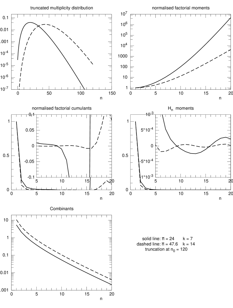
Figure 3: General behaviour of global observables $P_{n},\tilde{K}_{n},\tilde{F}_{n},H_{n}$ and $W_{n}$ as in Fig. 1 but for truncated NB (Pascal) MD’s.

Figure 4: General behaviour of global observables $P_{n},\tilde{K}_{n},\tilde{F}_{n}$ and $H_{n}$ as in Fig. 1 but for even-only NB (Pascal) MD’s (combinants are not shown as they are not relevant in this context.)

A second important application of $P_{0}(\Delta y)$ resides with jet production in hadron-hadron collisions: when jet production is associated with a colour-singlet exchange process, one expects a signature of rapidity gap events [53], while the production associated with colour-octet exchange (i.e., the one which is the focus of this review) will produce a much lower rate of empty rapidity intervals [54]. The difference between the two processes could lie in the different internal structure of clans [55]: in the colour-octet exchange, clans decay with a logarithmic distribution, as discussed in the previous section; in the colour-singlet exchange, clans decay with a geometric distribution. In other words, in both cases Eq. (59) remains valid, but with different values of $\bar{N}_{\text{g-clan}}$. It was found that such a scheme can describe well the excess of low multiplicity events in the colour-singlet exchange process [55].

2.4 CPMD’s, truncation and even-odd effects.

The maximum number of observed particles in the $n$ charged particle multiplicity distribution, $P_{n}$, never exceed a given number $n_{0}$, which of course increases with the c.m. energy of the collision. Theoretically, at least from energy-momentum conservation, this number is related to the available energy and the mass of the lightest charged particle, the pion. In experiments, there is in addition a practical limit (usually much lower than the theoretical one) related to the luminosity and total cross-section, i.e., dependent on the statistics. In order to guarantee that the probabilities sum to one, from the original (non-truncated) distribution $P_{n}$ a new MD is defined, $\tilde{P}_{n}$,

$$\tilde{P}_{n}=\begin{cases}AP_{n}&\text{if $n\leq n_{0}$}\\ 0&\text{if $n>n_{0}$}\end{cases},$$ (70)

such that $\sum_{n=0}^{n_{0}}\tilde{P}_{n}=1$. $A$ is the normalisation factor. It follows from their definition that factorial moments $F_{n}$ are equal to zero for $n>n_{0}$, whereas factorial cumulants $K_{n}$ are different from zero for any $n$. It should be pointed out that a truncated MD is not a CPMD and that at least one of its combinants $W_{n}$ is negative (for $n>n_{0}$.) Accordingly, factorial cumulants $F_{n}$ and the ratio of factorial cumulants to factorial moments, $H_{n}$, of a truncated MD are not positive definite. Notice that combinants of the truncated MD are not affected by the truncation process for $n<n_{0}$ (combinants are sensitive indeed to the head of the distribution and only to ratios $P_{n}/P_{0}$.) The truncation process becomes relevant for factorial cumulants, $K_{n}$, and for the ratio of factorial cumulants to factorial moments, $H_{n}$. This fact reflects the peculiar property of $K_{n}$ and $H_{n}$ to be sensitive to the tail of the MD. As an illustrative example, in Fig. 3 we present the same observables as in Fig. 1, for the case of a truncated NB (Pascal) MD. Of particular interest are the zeros of the generating function of a truncated MD (the GF in this case is a polynomial of order $n_{0}$).

Another conservation law which has to be obeyed is charge conservation: in annihilation events, only even multiplicities can be produced in FPS, while in narrow intervals this restriction is negligible (the so-called even-odd effect). One must also in this case re-normalise the MD:

$$\tilde{P}_{n}=\begin{cases}A^{\prime}P_{n}^{\text{(NBD)}}&\text{if $n$ is even}\\ 0&\text{if $n$ is odd}\end{cases}$$ (71)

so that $\sum_{n=0}^{\infty}\tilde{P}_{2n}=1$. For completeness, in Fig. 4 we present the same observables as in Fig.1 for a complete NB (Pascal) MD in which only even multiplicities are non-zero.

3 COLLECTIVE VARIABLES AND QCD PARTON SHOWERS

3.1 Parton showers in leading log approximation

Because our aim is to study the emission of soft gluons, fixed-order calculations in the coupling constant $\alpha_{s}$ are insufficient and a resummation of perturbative diagrams is needed. The standard approach [56] is to select the set of diagrams which dominate the perturbative series at high energies; since in the expansion one encounters physical amplitudes proportional to $\alpha_{s}^{n}(Q^{2})\log^{m}(Q^{2})$ with $m\leq n$, the leading terms are those in which $m=n$, which give the so-called leading log approximation (LLA).

In general, the factorisation theorem for collinear singularities allows to build a parton model description of the production process. For example, in the case of $e^{+}e^{-}$ annihilation into hadrons, the common wisdom suggests the following scheme (see Fig. 5): the electron and the positron annihilate into a virtual particle (a photon or a $Z^{0}$) which then decays into a quark-antiquark pair; this part is governed by the electroweak interaction theory. Perturbative QCD (pQCD) then describes the emission of further partons (mostly gluons) until the virtualities involved become too small: in this “soft region” where perturbation theory cannot be applied the produced partons merge with very soft gluons to form hadrons, often large mass resonances which then decay according to standard model rules.

Let us now go into more details: the single-inclusive cross section at hadron level $\sigma(\text{$e^{+}e^{-}$}\to hX)$ can be expressed in terms of a perturbative elementary cross-section $\sigma_{p}(\text{$e^{+}e^{-}$}\to q_{i}\bar{q}_{i})$ for a hard process at scale $Q^{2}$, and of a fragmentation function $D_{i}^{h}(z,Q^{2})$ which is interpreted as the probability of finding a hadron $h$ in the fragmentation of a parton of flavour $i$, carrying a fraction $z$ of the parton momentum:

$$\frac{d\sigma(\text{$e^{+}e^{-}$}\to hX)}{dz}=\sum_{i}\sigma_{p}(\text{$e^{+}e^{-}$}\to q_{i}\bar{q}_{i})D_{i}^{h}(z,Q^{2}),$$ (72)

where the sum runs over all flavours. Fragmentation functions, like structure functions in deep inelastic scattering, are universal and not calculable with perturbative methods. However, they can be expressed in terms of a $Q^{2}$-dependent partonic fragmentation function, $D_{i}^{j}(z,Q^{2},Q_{s}^{2})$, and a universal hadronic function at a fixed (soft) scale $Q_{s}$, $H_{j}^{h}(y,Q_{s})$,

$$D_{i}^{h}(z,Q^{2})=\sum_{j}\int_{0}^{1}\frac{dy}{y}D_{i}^{j}(z/y,Q^{2},Q_{s}^{2})H_{j}^{h}(y,Q_{s}).$$ (73)

Furthermore, the evolution with the hard scale can be calculated and is given by the Dokshitzer-Gribov-Lipatov-Altarelli-Parisi (DGLAP) equations:

$$\frac{dD_{i}^{j}(z,Q^{2})}{d\log Q^{2}}=\frac{\alpha_{s}(Q^{2})}{2\pi}\sum_{k}\int_{z}^{1}\frac{dx}{x}D_{k}^{j}(z/x,Q^{2},Q_{s}^{2})P_{jk}(x),$$ (74)

where $P_{jk}(z)$ is the DGLAP elementary kernel for the emission of parton $k$ from parton $j$, with parton $k$ carrying a fraction $z$ of $j$’s momentum. These kernels can be computed with elementary perturbative methods [56].

Figure 5: Schematic view of electron-proton annihilation into hadrons. (A) electroweak step (scale: $10^{-17}$ cm); (B) hard processes, described by perturbative QCD (scale: $10^{-15}$ cm); (C) soft non-perturbative processes (hadronization, scale: $10^{-13}$ cm); (D) decay of resonances into observable hadrons (mostly pions).

It is important to stress the simple physical meaning of DGLAP evolution equations in LLA: in the axial gauge, this approximation corresponds to select dressed ladder diagrams without interference terms and with strong ordering in the virtuality and transverse momentum of the offspring partons. It is this feature which allows to interpret the production process in a probabilistic language, in terms of a branching process. In this language, the elementary DGLAP kernel $P_{ab}(z)$ gives the probability density for a parton $a$ to emit a parton $b$ which carries a momentum fraction $z$.

Taking into account also the virtuality, we are led to a bi-dimensional elementary probability for the splitting of parton $a$ producing parton $b$ with momentum fraction $z$:

$$\frac{\alpha_{s}(Q^{2})}{2\pi}\frac{dQ}{Q}P_{ab}(z)dz.$$ (75)

In order to normalise this probability, one has to re-sum all virtual corrections, i.e., in the parton shower language, to take into account the probability that no parton is emitted at virtualities larger than $Q$; such probability is given by the Sudakov form factor:

$$S_{a}(Q|W)=\exp\left\{-\int_{Q^{2}}^{W^{2}}\frac{\alpha_{s}(K^{2})}{2\pi}\left[\sum_{b}\int_{z_{\text{min}}}^{z_{\text{max}}}P_{ab}(z)dz\right]\frac{dK^{2}}{K^{2}}\right\}.$$ (76)

Here the integration limits $z_{\text{min}}$ and $z_{\text{max}}$ depend on the kinematics of the splitting: this means that in general they (and consequently the whole expression in brackets) depend on the virtualities of both offspring partons and not only on $K$: this makes a closed form for $S_{a}(Q|W)$ impossible to find, unless some simpler approximation (like the fixed cut-off introduced below) is used.

Thanks to this probabilistic partonic picture, the result for single-inclusive distributions can be generalised using the “jet-calculus” rules [24] for $n$-parton fragmentation functions.

It should be noticed that both collinear and infrared singularities are present in the LLA expression of DGLAP kernels: the former ones are avoided by imposing a soft cut-off on the evolution ($Q_{s}>0$). The simplest way of curing infrared divergences is to impose a fixed (i.e., virtuality independent) cut-off on $z$, say $z_{\text{min}}\equiv\epsilon^{\prime}=1-z_{\text{max}}$; then one can simply interpret the integral of the regularized kernels as elementary splitting probabilities

$$A \equiv\int_{\epsilon^{\prime}}^{1-\epsilon^{\prime}}P_{gg}(z)dz=\frac{C_{a}}{\epsilon}=\frac{N_{c}}{\epsilon}$$ (77)

$$\tilde{A} \equiv\int_{\epsilon^{\prime}}^{1-\epsilon^{\prime}}P_{gq}(z)dz=\frac{C_{F}}{\epsilon}=\frac{N_{c}^{2}-1}{2\epsilon N_{c}}$$ (78)

$$B \equiv N_{f}\int_{\epsilon^{\prime}}^{1-\epsilon^{\prime}}P_{qg}(z)dz=\frac{N_{f}}{3}$$ (79)

with $\epsilon=(-2\ln\epsilon^{\prime})^{-1}$.

We will use the so-called “jet thickness” $\mathcal{Y}$ as evolution variable:

$$\mathcal{Y}=\frac{1}{2\pi b}\log\left(\frac{\alpha_{s}(Q^{2})}{\alpha_{s}(W^{2})}\right)=\frac{1}{2\pi b}\log\left(\frac{\log(W^{2}/\Lambda^{2})}{\log(Q^{2}/\Lambda^{2})}\right),$$ (80)

from virtuality $W$ down to $Q$, where $b=(11N_{c}-2N_{f})/12\pi$ and we used the leading order expression

$$\alpha_{s}(Q^{2})=\frac{1}{b\,\log(Q^{2}/\Lambda^{2})}.$$ (81)

Then the probability $P_{q}(Q|W)dQ$ that a quark of virtuality $W$ splits at a virtuality in the range $[Q,Q+dQ]$ (by emitting a gluon) is given by

$$P_{q}(Q|W)dQ=e^{-\tilde{A}\mathcal{Y}}\tilde{A}d\mathcal{Y},$$ (82)

and the probability $P_{g}(Q|W)dQ$ that a gluon splits (by either emitting another gluon or a quark-antiquark pair) by

$$P_{g}(Q|W)dQ=e^{-(A+B)\mathcal{Y}}(A+B)d\mathcal{Y}.$$ (83)

Neglecting conservation laws, the last two equations imply that the splitting probability is constant for each $d\mathcal{Y}$ interval: this allows to classify the process as Markovian, and therefore to write the appropriate forward and backward Kolmogorov equations for the probabilities to create $n_{q}$ quarks and $n_{g}$ gluons from an initial quark, $P_{q}(n_{q},n_{g};\mathcal{Y})$, or an initial gluon, $P_{g}(n_{q},n_{g};\mathcal{Y})$, at thickness $\mathcal{Y}$ [23]. The corresponding non-zero transition probabilities in an infinitesimal interval $d\mathcal{Y}$ are as follows:

$$\begin{split}(n_{q},n_{g})\to(n_{q},n_{g})\quad&=\quad 1-An_{g}d\mathcal{Y}-\tilde{A}n_{q}d\mathcal{Y}-Bn_{g}d\mathcal{Y};\\ (n_{q},n_{g})\to(n_{q},n_{g}+1)\quad&=\quad An_{g}d\mathcal{Y}+\tilde{A}n_{q}d\mathcal{Y};\\ (n_{q},n_{g})\to(n_{q}+2,n_{g}-1)\quad&=\quad Bn_{g}d\mathcal{Y}.\end{split}$$ (84)

It is simpler to use the generating functions (GF’s):

$$G_{a}(u,v;\mathcal{Y})\equiv\sum_{n_{q},n_{g}}u^{n_{q}}v^{n_{g}}P_{a}(n_{q},n_{g};\mathcal{Y})$$ (85)

where $a=q,g$. One obtains the following differential equations [23]:

$$\frac{dG_{g}}{d\mathcal{Y}} =A(G_{g}^{2}-G_{g})+B(G_{q}^{2}-G_{g}),$$ (86)

$$\frac{dG_{q}}{d\mathcal{Y}} =\tilde{A}G_{q}(G_{g}-1).$$ (87)

At low energy, the production of quark-antiquark pairs is negligible, and one can study solutions setting $B=0$: by looking only at the evolution of the number of gluons, the above equations decouple and the result is

$$G_{g}(u,v;\mathcal{Y}) =v[v+(1-v)e^{A\mathcal{Y}}]^{-1}$$ (88)

$$G_{q}(u,v;\mathcal{Y}) =u[v+(1-v)e^{A\mathcal{Y}}]^{-\tilde{A}/A}$$ (89)

The gluon multiplicity distribution (MD) in a gluon-initiated shower is found to be a shifted geometric distribution with average multiplicity $e^{A\mathcal{Y}}$ while the gluon MD in a quark initiated shower is a NB (Pascal) MD with average multiplicity $\bar{n}=\tilde{A}(e^{A\mathcal{Y}}-1)/A$ and parameter $k=\tilde{A}/A$, which for $\varepsilon$-regularization is just $(N_{c}^{2}-1)/2N_{c}^{2}$ (i.e., 4/9 with 3 colours). Clans in the quark jet case can be defined as in Section 2.2 and we obtain

$$\bar{N}=\tilde{A}\mathcal{Y};\quad\quad{\bar{n}_{c}}=\frac{e^{A\mathcal{Y}}-1}{A\mathcal{Y}}.$$ (90)

The two vertices: gluon production from a quark, controlled by parameter $\tilde{A}$, and gluon emission from a gluon, controlled by parameter $A$, have been separated and found to correspond respectively to clan production and gluon showers inside clans, in contrast to the standard parameterisation $\bar{n}$, $k$ where, as shown, the two vertices are mixed. This result leads to approximate clans to QCD bremsstrahlung gluon jets; gluons inside a clan follow on average a logarithmic distribution, which in turn can be written as a weighted average of the geometric distribution given in Eq. (88) (see Appendix A.4.)

To summarise, the essential conditions for the QCD interpretation of the occurrence of NB (Pascal) MD here discussed are: i) the independent emission of bremsstrahlung gluons, ii) the dominance of the vertex $g\to g+g$ over $g\to q+\bar{q}$, and iii) weak effects of coherence and conservation laws. The weakness of this approach is that it is very hard to introduce in the QCD Markov branching process the dependence on rapidity and therefore investigate MD’s far from full phase-space. We discuss in the next section some solutions to this problem.

3.2 The kinematics problem and possible answers.

In the treatment of the previous section, correct kinematics has not been taken into account: for example, at each splitting, phase-space is limited, as one should make sure that in $a\to b+c$, the virtualities sum up correctly: $Q_{a}\geq Q_{b}+Q_{c}$. Furthermore, energy and momentum conservation are not ensured. In order to address these problems, several methods have been developed: we will briefly mention the most popular of them, then discuss the simplified parton shower (SPS) and the generalised simplified parton shower (GSPS) models, which, although overlooked by the common wisdom, deserve in our opinion particular attention as an attempt to work in a fully correct kinematical framework by using essential features of QCD.

3.2.1 DLA and MLLA and Monte Carlo

In order to include more kinematics in the shower evolution, perturbations theory can be improved [56, 57, 58]. In the Double Log Approximation (DLA), for example, one takes into account the phase-space for the emission of a soft gluon; however, recoil is not considered for the parent parton, i.e., energy is not conserved in each individual emission. This can be justified in a first approximation by the hypothesis that emitted gluons are required to be soft, which is certainly applicable at asymptotic energies. Notice that DLA still allows a probabilistic interpretation of parton production as a cascade.

A noteworthy result in DLA is the prediction of Koba-Nielsen-Olesen (KNO) scaling [59] for the MD of gluons in a gluon jet; the high multiplicity tail is given by

$$f(n/\bar{n})\propto\exp(-Cn/\bar{n}),$$ (91)

where $C\approx 2.55$, calculated in pQCD. This KNO scaling form does not depend on the running of $\alpha_{s}$, being insensitive to all details of the evolution but the branching structure of the process ($\alpha_{s}$ of course appears in the energy dependence of $\bar{n}$.)

In order to bring into play also recoil effects, thus trying to solve the problem of the too prolific parton production of DLA, one arrives at the Modified Leading Log Approximation (MLLA) equations. Recoil effects modify the argument of evolution equations, taking the energy lost in the creation of a new parton into account. The equations become then differential equations with retarded terms (difference-differential equations). The probabilistic interpretation of the branching is still retained.

By considering only gluon production in a gluon-initiated jet, the DLA prediction has been corrected with pre-asymptotic terms, and the KNO scaling result is now violated at finite energies [60]. The new result for the tail is

$$f(n/\bar{n})\propto\exp[-(C^{\prime}n/\bar{n})^{\mu}],$$ (92)

where $\mu=(1-\gamma)^{-1}$ and $C^{\prime}=C\gamma^{\gamma}(1-\gamma)^{1-\gamma}/\Gamma(1+\gamma)$ and $\gamma=d\log\bar{n}/d\log Q$ is the anomalous dimension. MLLA predictions are much closer to experimental data than DLA ones, but the overall description is still poor, especially near the maximum. The tail is still close to an exponential (like that of a NB (Pascal) MD).

In addition to study the c.m. energy dependence of the MD, much can be learned from a study of its moments as a function of the order, at fixed energy. It was indeed found in [43] that it is possible to obtain analytic formulae within MLLA, even with the addition of higher order terms in an expansion in $\gamma$, in the limit of frozen $\alpha_{s}$, for the ratio $H_{q}$ of factorial cumulants to factorial moments. Numerical solutions [43] with running $\alpha_{s}$ have confirmed the oscillating behaviour of $H_{q}$ as a function of the order $q$ found analytically for solutions to the QCD equations for the generating functions. See Fig. 6. Oscillations of this type have been found experimentally, but before comparing to the pQCD predictions one has to take into account the truncation of the tail in the data (which was shown also to produce comparable oscillations [61]) and the effect of hadronization (actually, there is no effect when using generalised local parton-hadron duality, see Section 3.3.)

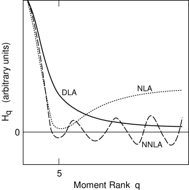
Figure 6: Ratio of cumulant to factorial moments, $H_{q}$, as function of the order $q$, computed in pQCD, using different approximations [62]: notice that ‘oscillations’ only appear in NNLA (dashed line).

In all analytical calculations however, while energy conservation is taken into account, momentum conservation is handled only by the angular ordering prescription; one then resorts to numerical methods, usually in terms of a Monte Carlo simulation of a parton shower: the evolution of partons can be traced step-by-step at each LLA vertex, imposing all conservation laws and required phase-space restrictions. Furthermore, not only multiplicities, but every aspect of the reaction may be simulated, although usually at the cost of adding extra parameters. It is remarkable that excellent results have been obtained in $e^{+}e^{-}$ annihilation into hadrons but not in minimum-bias $pp$ collisions, where general features like MD’s are still poorly described.

The Monte Carlo approach has been however particularly useful to obtain phenomenological ideas to be used in analytical calculations (see, e.g., Section 3.3 on hadronization.)

3.2.2 The SPS model

Another possibility to introduce kinematics constraints in QCD shower evolution is to isolate the fundamental features of pQCD on the basis of which a simplified analytical model can be developed in a correct kinematical framework. This is what has been attempted with the Simplified Parton Shower (SPS) model [63], described here in some detail.

We consider an initial parton of maximum allowed virtuality $W$ which splits at virtuality $Q$ into two partons of virtuality $Q_{0}$ and $Q_{1}$. We require $Q\geq Q_{0}+Q_{1}$ and $Q_{0},Q_{1}\geq 1$ GeV; this implies that any parton with virtuality less than 2 GeV cannot split further. We define the probability for a parton of virtuality $W$ to split at $Q$, $p(Q|W)$, which is normalised by a Sudakov form factor, as in Eq. (82) or (83). Since we are interested in the structure of the solution, we will discuss only one type of parton, introducing a free parameter which we call $A$, and use

$$p(Q|W)dQ=\frac{A}{Q}\frac{(\log Q)^{A-1}}{(\log W)^{A}}dQ=d\left(\frac{\log Q}{\log W}\right)^{A}.$$ (93)

The probability for an ancestor parton of maximum allowed virtuality $W$ to generate $n$ final partons, $P_{n}(W)$, and the probability for a parton which splits at virtuality $Q$ to generate $n$ final partons, $R_{n}(Q)$, with $P_{n}(Q)=R_{n}(Q)=\delta_{n1}$ for $Q<2$ GeV, lead to the following generating functions:

$$f(z,W)=\sum_{n=1}^{\infty}P_{n}(W)z^{n-1},$$ (94)

$$g(z,Q)=\sum_{n=2}^{\infty}R_{n}(Q)z^{n-2},$$ (95)

where the series has been shifted w.r.t. the standard definition in consideration of the fact that there is always at least one parton in the cascade; this definition will simplify some of the formulae to follow. The two generating functions are linked by

$$f(z,W)=\int_{1}^{2}p(Q|W)dQ+\int_{2}^{W}p(Q|W)zg(z,Q)dQ.$$ (96)

The joint probability density ${\mathcal{P}}(Q_{0}Q_{1}|Q)$ for a parton of virtuality $Q$ to split into two partons of virtuality $Q_{0}$ and $Q_{1}$ is defined by

$${\mathcal{P}}(Q_{0}Q_{1}|Q)=p(Q_{0}|Q)p(Q_{1}|Q)K(Q)\theta(Q-Q_{0}-Q_{1}),$$ (97)

where $K(Q)$ is a normalisation factor and the conditions on the virtualities are shown explicitly. The dynamical content of the model in virtuality is expressed by the following equation

$$R_{n}(Q)=\sum_{n^{\prime}=1}^{n-1}\int_{1}^{\infty}dQ_{0}\int_{1}^{\infty}dQ_{1}{\mathcal{P}}(Q_{0}Q_{1}|Q)R_{n-n^{\prime}}(Q_{0})R_{n^{\prime}}(Q_{1}),$$ (98)

which gives the probability for a parton which splits at virtuality $Q$ to generate $n$ final partons in terms of the joint probability density, Eq. (97), and of daughter parton’s respective showers.

Figure 7: Kinematically allowed virtuality domain in the SPS model for a parton splitting at virtuality $Q$ producing two offspring partons of virtualities $Q_{0}$ and $Q_{1}$, with $Q_{0}+Q_{1}<Q$. he dashed line indicates the extension of phase space due to the violation of the virtuality conservation law; the dotted lines indicate the domain in which only one of the two offsprings can split further [39].

Eq. (98) can be reformulated for the corresponding generating function by dividing the domain of integration in three sub-domains; one obtains

$$\begin{split}g(z,Q)&=\int_{1}^{2}dQ_{0}\int_{1}^{2}dQ_{1}{\mathcal{P}}(Q_{0}Q_{1}|Q)\\ &\quad+2\int_{1}^{2}dQ_{0}\int_{2}^{\infty}dQ_{1}{\mathcal{P}}(Q_{0}Q_{1}|Q)zg(z,Q_{1})\\ &\quad+\int_{2}^{\infty}dQ_{0}\int_{2}^{\infty}dQ_{1}{\mathcal{P}}(Q_{0}Q_{1}|Q)zg(z,Q_{0})zg(z,Q_{1}).\end{split}$$ (99)

The above three sub-domains correspond to the possible different situations in which the two generated partons can be found, i.e., neither of them splits, only one parton splits, or both partons split (see Figure 7.) This general scheme is valid for any choice of splitting function $p(Q|W)$, but in the present case this function factorizes and Eq. (96) simplifies into the differential equation

$$\frac{\partial f(z,W)}{\partial W}=p(W|W)[zg(z,W)-f(z,W)].$$ (100)

This equation can be easily solved in two extreme cases, obtained respectively by restricting or by relaxing phase-space constraints.

In the first case we allow to generate only very soft partons: $\theta(Q-Q_{0}-Q_{1})\to\theta(Q-Q_{0})\theta(2-Q_{1})$. This results in bremsstrahlung-like emission and a Poisson distribution of generated partons:

$$f(z,W)=e^{\lambda(W)(z-1)},$$ (101)

where

$$\lambda(W)=\int_{2}^{W}p(Q|Q)dQ=A\log\left(\frac{\log W}{\log 2}\right)$$ (102)

gives the average multiplicity of generated partons (in addition to the initial ancestor).

The second case is obtained by decoupling the virtualities as in $\theta(Q-Q_{0}-Q_{1})\to\theta(Q-Q_{0})\theta(Q-Q_{1})$. This is exactly the case examined for the LLA with fixed cut-off, Eq. (88), and indeed the result is a geometric distribution

$$f(z,W)=\left[1-(z-1)(e^{\lambda(W)}-1)\right]^{-1},$$ (103)

with average multiplicity of generated partons $e^{\lambda(W)}-1$.

Further analytical solutions of the SPS model were not possible, but numerical solutions using Monte Carlo methods show that the NB (Pascal) MD describes the MD’s rather well [63], which is not surprising considering that the NB (Pascal) MD interpolates between the Poisson ($1/k=0$) and the geometric ($k=1$) distributions.

Moreover, by differentiating the above equations for generating functions in $z=1$, one can obtain equations for factorial moments which are linear in the moments themselves, although they contain all moments of lower order. This feature, common to other evolution equations, is a consequence of the parton shower structure. But because the SPS model implements a correct kinematical framework, at small virtualities the equation simplify and a recursive solution can be achieved. Such a solution has to be numerical, but it was found [39] that the virtuality evolution is consistent with pQCD results and experimental observations for values of the parameter $A$ between 1.5 and 2. The behaviour of high order factorial moments qualitatively agrees with experimental data and with the most detailed pQCD calculations and is still consistent with NB (Pascal) predictions.

For describing the rapidity structure of the model, we propose to use the singular part of the QCD kernel controlling gluon branching:

$$p(y_{0}|Q_{0}Q_{1}Qy)\propto P(z_{0})dz_{0}\propto\frac{dz_{0}}{z_{0}(1-z_{0})}$$ (104)

Here $z_{0}$ is the energy fraction carried away by the produced parton in the infinite momentum frame.

The limits of variation of $z_{0}$ are fixed by the exact kinematical relations

$$B-\sqrt{B^{2}-\left(\frac{Q_{0}}{Q}\right)^{2}}\leq z_{0}\leq B+\sqrt{B^{2}-\left(\frac{Q_{0}}{Q}\right)^{2}},$$ (105)

where $B=\frac{1}{2}[1+({Q_{0}}/{Q})^{2}-({Q_{1}}/{Q})^{2}]$ is the scaled parton energy in the centre of mass system and $\sqrt{B^{2}-(Q_{0}/Q)^{2}}$ its maximum scaled transverse momentum. In this way the scaled transverse momentum (w.r.t. the parent direction) of the parton with energy fraction $z_{0}$

$$\frac{|p\kern-0.2pt\lower 4.0pt\hbox{\tiny T}_{0}|^{2}}{Q^{2}}=\sqrt{B^{2}-\left(\frac{Q_{0}}{Q}\right)^{2}}-(z_{0}-B)^{2}$$ (106)

and its rapidity

$$y_{0}=y+\frac{1}{2}\log\frac{z_{0}}{2B-z_{0}}$$ (107)

are uniquely determined. Rapidity of the second parton of virtuality $Q_{1}$ is obtained by energy-momentum conservation:

$$y_{1}=y+{\tanh}^{-1}\ \left[\frac{B}{B+1}{\tanh}\ |y_{0}-y|\right].$$ (108)

Notice that only the first step has to be treated differently in rapidity because it corresponds to the degrading from the maximum allowed virtuality $W$ to the virtuality of the first splitting $Q$. In this case the rapidity of the ancestor is fixed by conservation laws and is given by

$$y={\tanh}^{-1}\ \sqrt{1-\left(\frac{Q}{W}\right)^{2}}.$$ (109)

Again an analytical solution was not possible, but good fits to the Monte Carlo implementation of the SPS model in rapidity intervals were obtained with the NB (Pascal) MD.

3.2.3 The GSPS model: generalised clans

At this level of investigation, it should be clear that still open problems are the lack of the analytical solution of Eq. (99) and, in more general terms, the lack of a complete analytical study of the parton evolution process in rapidity.

In order to solve part of these problems, we proposed to incorporate in the SPS model the idea of clans; we called this version of the model “Generalised Simplified Parton Shower” (GSPS) model [64, 65]. Accordingly, we decided to pay attention for each event to the ancestor which, splitting $n$ times, gives rise to $n$ subprocesses (one at each splitting, see Fig. 8) and we identify them with clans. Therefore in this model for a single event the concept of clan at parton level is not a statistical one, as it was in the SPS model: in the present picture the clans are independent active parton sources and their number in each event coincides with the number of splittings of the ancestor, i.e., with the number of steps in the cascade.

Figure 8: The structure of the Generalised Simplified Parton Shower model (GSPS) for clan production in virtuality $Q$ and rapidity $y$. The production process is decoupled at each splitting both in virtuality and in rapidity, see Eqs. (112) and (114). Each blob represents a clan. Notice that here $Q_{0}\leq Q$, $Q_{1}\leq Q$, $|y_{0}-y|\leq\log{Q/Q_{0}}$, $|y_{1}-y|\leq\log{Q/Q_{1}}$ [64].

Notice that each clan generation is independent of previous history (it has no memory); thus the process is Markovian. Furthermore each generation process depends on the evolution variable only and is independent of the other variables of the process like the number of clans already present and their virtualities. In the original version of the SPS model, the splitting function of the first step, $p(Q_{0}|Q)$, was different from the splitting function of all the other steps, $\beta(Q_{0}|Q)$, obtained by integrating the joint probability function $\mathcal{P}(Q_{0},Q_{1}|Q)$,

$$\beta(Q_{0}|Q)=\int_{1}^{Q-Q_{0}}dQ_{1}\mathcal{P}(Q_{0},Q_{1}|Q).$$ (110)

In order to generalise the SPS model as it stands we assume that virtuality conservation law is locally violated (although conserved globally) according to

$$1\leq Q_{0}\leq Q,\qquad 1\leq Q_{1}\leq Q.$$ (111)

The upper limit of integration of Eq. (110) becomes $Q$, the normalisation factor $K(Q)$ reduces to 1 and the process becomes homogeneous in the evolution variable since

$$\beta(Q_{0}|Q)=p(Q_{0}|Q)\int_{1}^{Q}p(Q_{1}|Q)dQ_{1}=p(Q_{0}|Q).$$ (112)

The approximation described by this equation, therefore, can be interpreted as the effect of local fluctuations in virtuality occurring at each clan emission.

This violation of the virtuality conservation law spoils of course the validity of the energy-momentum conservation law, which, in the SPS model, uniquely determines the rapidity of a produced parton, given its virtuality and the virtuality and rapidity of its germane parton –see Eq. (108). In the GSPS model the two produced partons at each splitting are independent both in virtuality and in rapidity; however, the rapidity of each parton is bounded by the extension of phase-space fixed by its virtuality and the virtuality of the parent parton:

$$|y_{i}-y|\leq\log\frac{Q}{Q_{i}}.$$ (113)

In conclusion, by weakening locally conservation laws, we decouple the production process of partons at each splitting. Consequently, the GSPS model allows to follow just a branch of the splitting, since each splitting can be seen here as the product of two independent parton emissions. This consideration will be particularly useful in discussing the structure in rapidity of the model; in fact, it is implied that the DGLAP kernel given in Eq. (104) should be identified with

$$p(y_{0}|Q_{0}Qy)dy_{0}p(y_{1}|Q_{1}Qy)dy_{1}\propto\frac{dz_{0}}{z_{0}}\frac{dz_{1}}{z_{1}}.$$ (114)

Then one gets the multiplicity distribution $p_{N}(W)$:

$$p_{N}(W)=e^{-\lambda(W)}\frac{[\lambda(W)]^{N-1}}{(N-1)!},\qquad N>0.$$ (115)

Eq. (115) is a shifted Poisson distribution in the number of clans $N$, with average number of clans given by:

$$\bar{N}(W)=\sum_{N=1}^{\infty}Ne^{-\lambda(W)}\frac{[\lambda(W)]^{N-1}}{(N-1)!}=\lambda(W)+1.$$ (116)

We stress that this result has been obtained a priori in the present generalised version of the model, differently from what has been done previously in [66] where the independent production of clans was introduced a posteriori in order to explain the occurrence of NB (Pascal) regularity.

Since clans are by definition not correlated (i.e., only particles belonging to the same clan are correlated, while particles belonging to different clans are not) the MD of clans in rapidity intervals is obtained by binomial convolution

$$p_{N}(\Delta y,W)=\sum_{N^{\prime}=N}^{\infty}\binom{N^{\prime}}{N}\pi^{N}(1-\pi)^{N^{\prime}-N}p_{N^{\prime}}(W),$$ (117)

where $\pi(\Delta y,W)$ is the probability that one clan is produced within the interval $\Delta y$ by an ancestor parton of maximum virtuality $W$. The average number of clans in the interval $\Delta y$ is therefore

$$\bar{N}(\Delta y,W)=\pi(\Delta y,W)\bar{N}(W).$$ (118)

In terms of generating functions

$$F_{\text{clan}}(z;\Delta y)=\left[z\pi(\Delta y,W)+1-\pi(\Delta y,W)\right]e^{\pi(\Delta y,W)\lambda(W)(z-1)}.$$ (119)

Presenting the sum of two Poissonian distribution (the first a shifted one), this relations has a nice physical meaning: the two terms correspond to the probability of having the ancestor within or outside the given rapidity interval. When $\Delta y$ is very small, $\pi(\Delta y,W)$ tends to zero and the unshifted Poissonian dominates. Thus, it can be stated that in the smallest rapidity intervals the clan multiplicity is to a good approximation Poissonian and the full MD belongs to the class of Compound Poisson Distribution. $\pi(\Delta y,W)$ tends to 1 for large $\Delta y$ and the exact full phase-space shifted-Poisson distribution is approached. Finally, when $\pi(\Delta y,W)\lambda(W)$ is sufficiently large, the shifted-Poissonian dominates at large $N$ (the tail of the distribution) while the unshifted one dominates at small $N$ (the head of the distribution). These facts might have some consequences in interpreting the anomalies found in NB behaviour for small $N$ and the deviations from NB behaviour in large rapidity intervals, which are controlled by the behaviour of the distribution at large $N$.

The calculation of $\bar{N}(\Delta y,W)$ can then be carried out analytically, although the procedure is very tedious. The key observation is that, thanks to the decoupling, the elementary splitting function for an ancestor parton of virtuality $Q$ to produce a clan of virtuality $Q_{1}$ has the same functional form of the probability that the next splitting of the ancestor itself happens at virtuality $Q_{0}$. Therefore, the ancestor and the clan at the last step of the shower evolution can be interchanged. We will skip the details of the calculation, to be found in [64], and proceed to illustrate the results.

In Fig. 9 the clan density is shown as a function of the width of the interval $\Delta y\equiv[-y_{c},y_{c}]$ for $A=2$ for maximum allowed virtualities $W=50$ GeV, $W=$ 100 GeV and $W=500$ GeV. The contribution of one-parton showers turns out to be negligible for this choice of $A$. Notice that the height of the distribution is decreasing (simply because the full phase-space value increases only as a double log) and the width increasing with the energy (phase-space grows logarithmically). Convolution of clan density for two back-to-back parton showers is shown in Fig. 10. Notice that the central dip at $y\simeq 0$ is slowly removed by increasing the energy of the initial parton. It should be kept in mind that the structure of Figures 9 and 10 refers to clan production; the different behaviour for parton production inferred from data is not in contradiction with this behaviour since we have still to include in our scheme parton production within a single clan.

In Figure 11 the average number of clans $\bar{N}(\Delta y,W)$ is given as a function of rapidity width $y_{c}$ for the same $W$ values of Figure 9. Limitations on the rapidity intervals are determined by the available phase-space corresponding to the different initial parton virtualities.

Figure 9: Clan density in rapidity, i.e., number of clans per unit rapidity, in a single parton shower, according to the GSPS model with parameter $A=2$. The three curves refer to different initial virtualities (dotted line: $W=50$ GeV; dashed line: $W=100$ GeV; solid line: $W=500$ GeV) and are normalised each to its own average number of clans in full phase-space [64].

Figure 10: Clan density in rapidity resulting by the addition of two back-to-back showers, at different initial virtualities in the GSPS model [64]. All parameters as in Fig. 9

Figure 11: Average number of clans in a central rapidity interval $[-y_{c},y_{c}]$ as a function of the interval’s half-width $y_{c}$ for a single shower in the GSPS model with $A=2$. The three curves refer to different initial virtualities (dotted line: $W=50$ GeV; dashed line: $W=100$ GeV; solid line: $W=500$ GeV) [64].

Figure 12: The same curves as in Fig. 11, rescaled in the abscissa to the respective full phase-space (FPS) rapidity and in the ordinate to the respective FPS average number of clans, i.e., Eq. (120) vs. $y_{c}^{*}=y_{c}/y_{\text{fps}}$ [64].

Accordingly, the GSPS model predicts, for the average number of clans at parton level in a single shower (jet):

1. a rise with the rapidity width $y_{c}$, for different initial parton virtualities $W$, which is very close to linear for $1<y_{c}<y_{\text{fps}}$; the rise is still linear but with a somewhat different slope for $y_{c}<1$. A characteristic bending occurs finally for rapidity width $y_{c}\lesssim y_{\rm fps}$;

2. approximate (within 5%) energy independence in a fixed rapidity interval $y_{c}$ for $W$ below 100 GeV. For higher virtualities, deviations from energy independence become larger; they are within 20% when comparing $\bar{N}(y_{c},50\ {\text{GeV}})$ and $\bar{N}(y_{c},500\ {\text{GeV}})$. It should be noticed that the average number of clans slowly decreases with virtuality; this behaviour has been already observed in Monte Carlo simulations for single gluon jets [67].

In addition to the above results which are consistent with our expectations on clan properties in parton showers, the model shows energy independent behaviour (see Figure 12) by normalising the average number of clans produced in a fixed rapidity interval $|y|\leq y_{c}$ to the corresponding average number in full phase-space, and by expressing this ratio as a function of the rescaled rapidity variable $y_{c}^{*}\equiv y_{c}/y_{\rm fps}$:

$$\pi^{*}(y_{c}^{*},W)\equiv\frac{\bar{N}(y_{c}^{*}\ y_{\rm fps},W)}{\bar{N}(W)}$$ (120)

This new regularity turns out to be stable for different choices of the parameter $A$. In Figure 12 a clean linear behaviour is shown for the above ratio corresponding to the parameter value $A$=2.

Having completed the analytical treatment of the number of clans, we now proceed to the final partons level. In order to study the average number of clans in the rapidity interval $\Delta y$, $\bar{N}(\Delta y,W)$, in the previous treatment we limited our discussion to the first step of parton shower evolution in the GSPS model. It is clear that if one wants to calculate the average number of partons per clan in the same interval, $\bar{n}_{c}(\Delta y,W)$, one has to analyse the second step of parton shower evolution, i.e., to study the production of partons inside clans. In order to do that, inspired by the criterion of simplicity and previous findings, we decided to maintain inside a clan the structure of the model seen in the first step. The only difference lies in the introduction of a new parameter, $a$, controlling the length of the cascade inside a clan, in the expression of the probability that a parton of virtuality $Q$ emits a daughter parton in the virtuality range [$Q_{0},Q_{0}+dQ_{0}$], i.e.,

$$p_{a}(Q_{0}|Q)dQ_{0}=d\left(\frac{\log Q_{0}}{\log Q}\right)^{a}\;.$$ (121)

The GSPS model is thus a two-parameter model: $A$ and $a$, controlling the length of the cascade in step 1 and 2 respectively. This is equivalent to introducing the SPS structure for a single clan; however, by maintaining the decoupling in each splitting (a la DLA) one keeps the possibility to solve the model exactly.

The MD in a clan of virtuality $Q$ is therefore

$$g_{\text{fps}}(z,Q)=\begin{cases}\frac{z}{1+(\bar{n}_{c}(Q)-1)(1-z)}&Q\geq 2\ {\text{GeV}}\\ z&Q<2\ {\text{GeV}}\end{cases}$$ (122)

where

$$\bar{n}_{c}(Q)=e^{\lambda_{a}(Q)}\;,\qquad\lambda_{a}(Q)=\int_{2}^{Q}p_{a}(Q^{\prime}|Q^{\prime})dQ^{\prime}\;.$$ (123)

The solutions correspond to a shifted geometric distribution ($Q\geq 2$ GeV) and to a clan with only one parton ($Q<2$ GeV). The bound 2 GeV is a consequence of the fact that in the GSPS model the virtuality cut-off is fixed at 1 GeV (a parton with virtuality $Q<2$ GeV cannot split any further by assumption). Notice that this finding agrees with the clan model discussed in [68], where the logarithmic MD for partons inside average clans is interpreted as the result of an average over geometrically distributed single clans of different multiplicity, i.e., initial virtuality (See also Appendix A.4.)

We now calculate the generating function of partons MD in a rapidity interval $\Delta y$ inside a clan of virtuality $Q$ and rapidity $y$: this is done through a binomial convolution on the corresponding generating function in full phase-space:

$$g_{\Delta y}(z,Q,y)=\begin{cases}\frac{1+(z-1)\pi_{a}(\Delta y,Q,y)}{1+\pi_{a}(\Delta y,Q,y)(\bar{n}_{c}(Q)-1)(1-z)}&Q\geq 2\ {\text{GeV}}\\ 1+(z-1)\pi_{a}(\Delta y,Q,y)&Q<2\ {\text{GeV}}\end{cases}$$ (124)

where $\pi_{a}(\Delta y,Q,y)$ is the probability that a clan of initial virtuality $Q$ and rapidity $y$ produces a daughter parton inside the interval $\Delta y$. Notice that this approximation neglects rapidity correlations among particles in the same clan. However, it allows exact analytical solutions (although long and cumbersome to handle). The average number of partons per clan is then

$${\bar{n}_{c}}(\Delta y,Q,y)=\pi_{a}(\Delta y,Q,y)e^{\lambda_{a}(Q)}.$$ (125)

When the above equation is averaged over the probability that a parton of maximum allowed virtuality $W$ produces a clan of virtuality $Q$ and rapidity $y$, we obtain the average number of partons in an average clan generated in a shower of virtuality $W$. As probability over which we average, one can use the bi-dimensional clan density in virtuality and rapidity normalised by the average number of clans. Results of the calculations of the average number of particles per clan as a function of the rapidity interval $\Delta y$ and of the maximum allowed virtuality $W$ with $A=2$ and $a=1$ are shown in Fig. 13 for $W$= 50 GeV (solid line), $W$=100 GeV (dashed line) and $W$= 500 GeV (dotted line). The trend fully coincide with the behaviour of clans structure parameters obtained by analysing quark and gluon jets MD’s [67]. The result of the analytical calculation of the average number of partons in the shower, $\bar{n}(\Delta y,W)$ is shown in Figure 14 with the same parameters. The average parton multiplicity grows almost linearly with rapidity for relatively small $\Delta y$ intervals and then it is slowly bending for $\Delta y$ intervals approaching f.p.s., where it reaches its maximum. It is interesting to remark that the normalised average number of partons in the shower, $\bar{n}(\Delta y,W)/\bar{n}({\text{fps}},W)$ scales in virtuality as a function of the rescaled rapidity interval, $\Delta y/{\text{fps}}$, see Figure 15. This scaling in $W$ is found to depend on the parameter $a$, as different values of $a$ give different scaling curves, differently from the scaling found for for $\bar{N}(\Delta y,W)/\bar{N}({\text{fps}},W)$ which is independent of the mechanism inside clans.

Figure 13: Average number of partons per clan in a central rapidity interval $[-y_{c},y_{c}]$ as a function of the interval’s half-width $y_{c}$ for a single shower in the GSPS model with $A=2$, $a=1$. The three curves refer to different initial virtualities (dotted line: $W=50$ GeV; dashed line: $W=100$ GeV; solid line: $W=500$ GeV) [65].

Figure 14: Average number of partons in a central rapidity interval $[-y_{c},y_{c}]$ as a function of the interval’s half-width $y_{c}$ for a single shower in the GSPS model with $A=2$, $a=1$. The three curves refer to different initial virtualities (dotted line: $W=50$ GeV; dashed line: $W=100$ GeV; solid line: $W=500$ GeV) [65].

Figure 15: Same curves as in Fig. 14, rescaled in abscissa to the respective FPS rapidity, and in ordinate to the respective average FPS multiplicity [65].

In conclusion, the GSPS model is a parton shower model which was built assuming QCD-inspired dependence of the splitting functions in virtuality and in rapidity, with Sudakov form factors for their normalisation; in addition to these ingredients (which were called “essentials of QCD”), the characterising feature was introduced of distinguishing explicitly the two steps of clan production and subsequent decay, allowing at each step in the cascade local violations of energy-momentum conservation laws but requiring its global validity. This model was found to have an important predictive power in regions not accessible to pQCD. Analytical calculations of the virtuality and rapidity dependence of the average number of clans and of the average number of particles per clan have been carried out. Results are consistent with what is known on clan properties in single quark and gluon jets, disentangled at hadron level by using jet finding algorithms and analysed at parton level assuming that generalised local parton-hadron duality (discussed in the next Section) is applicable.

3.3 Hadronization prescriptions

Having performed computations at parton level, the problem arises on how to make the connection with the measured hadron level. Such a process is of course non-perturbative in nature, and usually approached through various models: the string model [69] and the cluster model [70] are widely used in Monte Carlo calculations; statistical hadronisation models [71] are now starting to know considerable success.

It has been noticed however that many predictions of perturbation theory can reproduce experimental results down to low virtuality scales, and often give the correct energy evolution except for an overall normalisation. This behaviour can be expressed in terms of pre-confinement: the perturbative evolution is continued to low virtualities while partons rearrange themselves in their evolution to form colour singlet clusters which hadronize subsequently at a soft scale of the order of the perturbative cut-off to the shower. This picture lead to the Local Parton-Hadron Duality (LPHD, ‘weak’ duality) prescription: single-particle inclusive distributions at hadron level are taken proportional to the corresponding distribution at parton level:

$$Q_{1}^{(h)}(y)=\rho Q_{1}^{(p)}(y),$$ (126)

where in general $\rho\approx 2$. It is a way to investigate to what extent pQCD can directly reproduce experimental data up to a rescaling factor. In particular, integrating Eq. (126) one obtains for the average multiplicities:

$$\bar{n}^{(h)}=\rho\bar{n}^{(p)}.$$ (127)

In [26], it was noticed in that Monte Carlo calculations of MD’s, the NB (Pascal) MD provided a good fit both at parton and hadron level, with the same parameter $k$. This lead to the formulation of Generalised LPHD (GLPHD; ‘strong’ duality) which brings into play higher order inclusive distributions:

$$Q_{n}^{(h)}(y_{1},\dots,y_{n})=\rho^{n}Q_{n}^{(p)}(y_{1},\dots,y_{n}).$$ (128)

In general, one expects $\rho>1$. Integrating over rapidity, one obtains the proportionality of (un-normalised) factorial moments:

$$F_{n}^{(h)}=\rho^{n}F_{n}^{(p)};$$ (129)

recalling Eq. (26) which links factorial moments with generating functions, one obtains the relation:

$$G^{(h)}(z)=G^{(p)}(1-\rho+\rho z).$$ (130)

This relation leaves unchanged all the observables that do not depend on the average multiplicity. It can easily be seen, e.g., that normalised factorial moments are the same at parton and hadron level, being $F_{1}^{(h)}=\rho F_{1}^{(p)}$. The same is true for normalised factorial cumulant moments, since they can be expressed as a sum over factorial moments (recall the cluster expansion that links inclusive distributions to correlation functions, Eq. (8). Of course, it follows that also the ratio $K_{n}/F_{n}=H_{n}$ is invariant under the GLPHD transformation:

$$K_{n}^{(h)} =\rho^{n}K_{n}^{(p)};$$ (131)

$$H_{n}^{(h)} =K_{n}^{(h)}/F_{n}^{(h)}=K_{n}^{(p)}/F_{n}^{(p)}=H_{n}^{(p)}.$$ (132)

When applying Eq. (130) to MD’s which are infinitely divisible at parton level, one still obtains (barring pathological cases) distributions which are CPMD’s:

$$G^{(h)}(z)=\exp\{\bar{N}^{(p)}[g^{(p)}(1-\rho+\rho z)-1]\}.$$ (133)

However, at $z=0$ one obtains $g^{(p)}(1-\rho)\neq 0$, which violates the condition that there are no empty clans. One has to redefine the MD within clans [72, 73]:

$$g^{(h)}(z)=\frac{g^{(p)}(1-\rho+\rho z)-g^{(p)}(1-\rho)}{1-g^{(p)}(1-\rho)}.$$ (134)

This is equivalent to the following transformation on the clan parameters:

$$\bar{N}^{(h)} =\bar{N}^{(p)}\left[1-g^{(p)}(1-\rho)\right],$$ (135)

$${\bar{n}_{c}}^{(h)} ={\bar{n}_{c}}^{(p)}\frac{\rho}{1-g^{(p)}(1-\rho)}.$$ (136)

Because (in reasonable situations) $g^{(p)}(1-\rho)\leq 0$, one has $\bar{N}^{(h)}\geq\bar{N}^{(p)}$. It is interesting to remark that hadronic clans do not coincide with the partonic ones: hadronisation creates in general new clans (or breaks partonic ones) [74]. Indeed one also has ${\bar{n}_{c}}^{(h)}\geq{\bar{n}_{c}}^{(p)}$. The exact sharing of the multiplicity increase between $\bar{N}$ and ${\bar{n}_{c}}$ depends on the actual shape of $g^{(p)}(z)$.

As an example, in the case of the NB (Pascal) MD we obtain that GLPHD is equivalent to the following simple requirement:

$$\bar{n}^{(h)}=\rho\bar{n}^{(p)}\quad,\qquad k^{(h)}=k^{(p)}:$$ (137)

notice the NB(Pascal) shape is not lost, only one parameter changes when going from the partonic to the hadronic level. In this example, both the average number of clans and the average number of partons (particles) per clan increase during hadronization:

$$\bar{N}^{(h)} =k^{(p)}\ln\left(1+\rho\bar{n}^{(p)}/k^{(p)}\right),$$ (138)

$${\bar{n}_{c}}^{(h)} =\frac{\rho\bar{n}^{(p)}}{k^{(p)}\ln\left(1+\rho\bar{n}^{(p)}/k^{(p)}\right)}.$$ (139)

It is worth pointing out that GLPHD has some drawbacks: relation (130) resembles a convolution with a binomial distribution, except that $\rho>1$. On one hand this fact prevents a probabilistic interpretation of GLPHD: it is impossible to define event by event a probability distribution for obtaining $n$ particles from $m$ partons satisfying Eq. (130). On the other hand it allows to study the distributions that are invariant in form under transformation (130): they are all MD’s whose GF depends on $z$ and $\bar{n}$ only via the product $\bar{n}(z-1)$, i.e., which satisfy the following differential equation:

$$\bar{n}\frac{\partial G(z)}{\partial\bar{n}}=(z-1)\frac{\partial G(z)}{\partial z}.$$ (140)

This equation can be formally solved and gives, at the level of probabilities, Eq. (53) —see [39].

It should be clear by now that GLPHD is a very strong prescription, certainly too strong: there are effects present at hadronic level only (e.g., resonances’ decays) which affect hadronic correlations and not partonic ones; on the contrary, GLPHD fixes all correlations already at parton level (except for their overall strength). Nonetheless, GLPHD is very useful as a tool to investigate the predictive power of purely perturbative calculations: recall for example the case of $H_{q}$ moments oscillations.

4 COLLECTIVE VARIABLES REGULARITIES IN MULTIPARTICLE PRODUCTION: DATA AND PERSPECTIVES

The attempt to achieve a unified, QCD-inspired description of multiparticle production in all classes of collisions, in full phase-space and in its limited intervals, both at final hadron and parton level and from the soft sectors up to the hard ones, including high parton density regions, is the challenge in the field. The main motivation of the present section is the conviction —already stated in the introduction— that complex structure which we observe might very well be, at the origin, simple, and that such initial simplicity manifests itself in terms of regularities of final particle multiplicities. With this aim, it is instructive and stimulating —in our opinion— both from a theoretical and an experimental point of view, to follow the advent of the NB (Pascal) MD regularity and of KNO scaling violation in multiparticle production (facts which haven’t yet been fully appreciated in all their implications), then to see the sudden failure of the regularity as a consequence of the shoulder structure observed in $n$ charged particle MD’s $P_{n}$ when plotted vs. $n$, and finally its reappearance at a deeper level of investigation, i.e., in the description of the substructures or classes of events of the various collisions.

What makes even more attractive this development is the finding that, under certain reasonable assumptions, the NB (Pascal) MD occurs also (see Section 3) at final parton level: the generating function of the NB (Pascal) MD is the solution of the differential QCD evolution Equations which can be understood as a Markov branching process initiated by a parton and controlled in its development by QCD elementary probabilities. It should be noticed that the same regularity appears also in final $n$-parton multiplicity distributions in $q\bar{q}$ and $gg$ systems in Jetset 7.2 Monte Carlo calculations based on DGLAP equations. In addition, by using a convenient guesswork as hadronization prescription, the NB (Pascal) MD describes within the same Monte Carlo generator the hadron level, which turns out not to be independent from the parton level but linked to it by strong GLHP duality. All these results can be interpreted, as we shall see, in terms of clan structure analysis and suggest that the dynamical mechanism responsible of multiparticle production in all classes of collisions is independent intermediate gluon sources (the clan ancestors) emission followed by QCD parton shower formation.

4.1 An unsuspected regularity in particle production in cosmic ray physics

After the discovery of multiparticle production (groups of “mesotrons”) in cosmic rays in the thirties and the important theoretical work in the forties and early fifties in order to explain the highly non linear new phenomenon, the contribution of the 1966 paper by P.M. MacKeown and A.W. Wolfendale [11] should be mentioned. Its interest lies in the attempt to describe all available experimental data on exclusive $n$-particle cross sections, $\sigma_{n}{(E_{0})}$, for producing $n$ charged pions generated by a primary nucleon at different energies $E_{0}$ (from $25$ GeV up to $5\cdot 10^{4}$ GeV) by using a NB (Pascal) MD, i.e.

$$\sigma_{n}(E_{0})=\frac{\bar{n}^{n}}{n!}\left[1+\frac{\bar{n}}{k(E_{0})}\right]^{-n-k(E_{0})}\prod_{j=1}^{n-1}\left(1+\frac{j}{k(E_{0})}\right),$$ (141)

with $n=n_{s}-1$, $n_{s}$ being the number of shower tracks. According to the fits shown in Figure 16 one can conclude that particles in cosmic ray are not independently produced but are highly correlated. It should be noticed that the Authors of [11] determined also the energy dependence of the two standard parameters of the proposed phenomenological multiplicity distribution. They found

$$k^{-1}(E_{0})=0.4(1-\exp[-1.8\cdot 10^{-4}E_{0}])$$ (142)

and

$$\bar{n}=1.8E_{0}^{1/4}.$$ (143)

Particle correlations are controlled by $1/k$ and become stronger as the primary energy becomes larger. To the growth of $\bar{n}$ from 4.02 at primary energy $E_{0}=25$ GeV to 26.92 at $E_{0}=5\cdot 10^{4}$ it corresponds in the same energy range the decrease of $k$ parameter from 557 to 2.5 . This result is even more stimulating when interpreted in the framework of clan structure analysis: the average number of clans, $\bar{N}$, is growing from $\approx 4$ to 6.16 and the average number of particles per clan, $\bar{n}_{c}$, from $\approx 1.0$ to 4.37, indicating a strong clustering effect as the primary energy becomes larger (Table 1.)

Figure 16: MD of produced particles from a variety of experiments in cosmic ray vs the number of charged tracks $n_{s}$. The curves represent NB (Pascal) MD’s (a) $E_{0}=30$ GeV, (b) $E_{0}=25$ GeV, (c) $E_{0}=300$ GeV, (d) $E_{0}=1.5\cdot 10^{4}$ GeV, (e) $E_{0}=10^{4}$ GeV, where $E_{0}$ is the primary nucleon energy [11].

Table 1: NB (Pascal) MD parameters calculated at different primary nucleon energies $E_{0}$, using Eqs (142) and (143) [11].

$E_{0}$	$\bar{n}$	$k$	$\bar{N}$	${\bar{n}_{c}}$
25 GeV	4.02	557	4.01	1.0
30 GeV	4.21	464	4.19	1.0
300 GeV	7.49	47.6	6.96	1.08
1000 GeV	10.12	15.18	7.75	1.31
5000 GeV	15.14	4.21	6.42	2.36
$10^{4}$ GeV	18	3	5.84	3.08
$1.5\cdot 10^{4}$ GeV	19.92	2.68	5.71	3.49
$5\cdot 10^{4}$ GeV	26.92	2.5	6.16	4.37

4.2 The occurrence of the NB (Pascal) regularity in full phase-space in the accelerator region and the generalised multiperipheral bootstrap model.

In 1972 the KNO scaling violation and the widening of the $n$ charged particle MD with the increase of $p_{\text{lab}}$ are confirmed in hadron-hadron collisions in the accelerator region [19]. It is found that the NB (Pascal) MD describes $n$ charged particle MD’s, $P_{n}$, when plotted vs. $n$; to the increase with $p_{\text{lab}}$ of the average charged multiplicity $\bar{n}$ one notices the decrease of the parameter $k$, i.e., the dispersion $D=\sqrt{\langle\bar{n}^{2}\rangle-\langle\bar{n}\rangle^{2}}$ becomes larger in contrast with multiperipheral model predictions and in agreement with cosmic rays experimental findings. The inverse of $k$ NB parameter, $g^{2}\equiv k^{-1}$, is interpreted in the generalised multiperipheral bootstrap model [15] as the ratio between the pomeron-reggeon-particle vertex controlling diffraction phenomena ($g^{2}_{P}$) and the reggeon-reggeon particle vertex ($g^{2}_{M}$). $g^{2}$ is evaluated to vary between 0.01 at 30 GeV/c and 0.67 in the above mentioned extreme cosmic ray experiments. The occurrence of the NB distribution in the generalised multiperipheral bootstrap model is understood as the effect of the weighted superposition of $r$ multiperipheral diagrams with $\bar{n}_{r}={r\bar{n}}$ and $\bar{n}$ the average multiplicity of the first Poissonian multiperipheral diagram, i.e., $\bar{n}=g^{2}_{M}\ln(s/m_{a}m_{b})$ ($m_{a}$ and $m_{b}$ are the masses of the initial particles and $\sqrt{s}$ the c.m.energy). The distribution function which weights the average multiplicity in the set of multiperipheral diagrams is a function of $g^{2}$ and $r$ and is assumed to be a gamma distribution

$$f(r,g^{2})=\frac{(r/g^{2})^{(1-g^{2})/g^{2}}}{{(1-g^{2})/g^{2}}!}\exp(-r/g^{2}).$$ (144)

It follows

$$\sigma_{n}=\sigma_{\text{tot}}\int_{0}^{\infty}\frac{(r\bar{n})^{n}}{n!}\exp[-r\bar{n}]\frac{(r/g^{2})^{(1-g^{2})/g^{2}}}{{(1-g^{2})/g^{2}}!}\exp(-r/g^{2})d(r/g^{2}),$$ (145)

that is

$$\sigma_{n}=\sigma_{\text{tot}}\left(\frac{\bar{n}}{1+g^{2}\bar{n}}\right)^{n}\frac{(1+g^{2})\cdots\left(1+(n+1)g^{2}\right)}{n!}(1+g^{2}\bar{n})^{-1/g^{2}}.$$ (146)

Figure 17: NB (Pascal) MD (solid line) and Poisson (dashed line) formulae plotted vs. the number of charged particles $n$ compared with data on $pp$ collisions at different projectile momenta in the laboratory frame [14].

Figure 18: Overall $1/k$ data as a function of projectile momentum in the laboratory frame $p_{\text{lab}}$ for the reactions listed [14].

For $g^{2}_{P}=0$, $\bar{n}\approx g^{2}_{M}\ln(s/m_{a}m_{b})$ and

$$\sigma_{n}\approx\sigma_{\text{tot}}\bar{n}^{n}\frac{e^{-\bar{n}}}{n!}$$ (147)

and in general $1/k(s/s_{0})=g_{P}^{2}/g_{M}^{2}h(s/s_{0})$. From a purely phenomenological point of view, it should be pointed out that multiplicity distributions of available hadron-hadron collision experiments in the accelerator region were all successfully described by the NB (Pascal) MD (see for example Fig. 17) in a series of papers which were overlooked in the field. In addition, deviations from Poisson MD were interpreted as the onset of pomeron-reggeon vertex. Of particular interest was the fact that $k^{-1}$ parameter was increasing with c.m. energy in the accelerator region as in cosmic rays in all hadron-hadron reactions and crossing the zero point in the low energy domain (few GeV/c), as shown in Figure 18, in agreement with later findings [25, 75].

An alternative interpretation of the regularity in terms of a stochastic cell model was also suggested by one of the present Authors in 1973 [13] and then extensively discussed by P. Carruthers [76]. $k^{-1}$ parameter is understood in this framework as a stimulated emission factor, i.e., the fraction of particles already present stimulating the emission of an additional particle.

4.3 The advent of the regularity in different classes of collisions and in rapidity intervals, and its interpretation in terms of clans.

In 1985, the UA5 collaboration rediscovered NB (Pascal) MD for describing CERN $p\bar{p}$ collider MD data in full phase-space and in symmetric rapidity intervals [77] as shown in Fig. 19.

Figure 19: MD $P_{n}$ vs. $n$ in $p\bar{p}$ collisions at c.m. energy 546 GeV in different pseudo-rapidity intervals are shown together with fits using the NB (Pascal) MD (solid lines) [78].

Figure 20: Compilation of measurements of the average charged multiplicity $\bar{n}$ and of the normalised variance $D^{2}/\bar{n}^{2}$ in $pp$ and pp̄ collisions. Superimposed are interpolations to the NB (Pascal) MD parameters $\bar{n}$ and $k$ and their sum (the band takes into account interpolation errors) according to the NB relation $D^{2}/\bar{n}^{2}=1/k+1/\bar{n}$ [16].

Figure 21: Multiplicity distributions for final charged particles in various reactions but at similar c.m. energies; data are taken in central symmetric rapidity intervals $|y|<y_{c}$ and in full phase-space as shown by the labels. The lines are fits with NB (Pascal) MD [79].

In going from ISR and SERPUKHOV up to CERN $p\bar{p}$ Collider data [16, 80], $\bar{n}$ becomes larger and $k$ parameter smaller as the c.m. energy of the collision becomes larger, as shown in Figure 20, confirming the general trends of NB parameters already observed in the accelerator and in the cosmic ray regions. In addition, parameter $k$ is smaller in central pseudo-rapidity intervals, suggesting the onset of a significant dynamical effect in central regions not hidden by conservation laws, and indicating stronger particle correlations with respect to the larger intervals where conservation laws are the dominant effect (see [81] for a detailed review).

The next question concerned the possible extension of the regularity to other classes of collisions, both in the available energy domain and in symmetric (pseudo)-rapidity intervals. The answer came from NA22, EMC and TASSO collaborations as shown in Figure 21. $P_{n}$ vs. $n$ data were very well fitted by NB (Pascal) MD’s in hadron-hadron [17], lepton-hadron [21] and lepton-lepton [18] collisions at nearly the same c.m. energy both in FPS and in (pseudo)-rapidity intervals. The success of the regularity in describing $n$ charged particle MD’s in all classes of collisions and in symmetric rapidity intervals, i.e., its universality, demanded an interpretation in more physical terms. Previous phenomenological models, although leading to the experimentally observed $n$ charged particle multiplicity distribution, were too poor and in a certain sense too naive for the new wide domain of validity of the regularity, especially in view also of the almost simultaneous achievements of QCD as the theory of strong interactions. This search was developed in two moments.

Firstly the characterisation of the observed regularity at hadron level in more physical terms was studied. Cascading and stimulated emission appeared as the natural candidates for the dynamical mechanisms leading to the observed distribution. It is interesting to point out that, according to the interpretation of $k^{-1}$, in the stimulated emission framework $k^{-1}$ should be always larger than or equal to 1. Since stimulating emission was excluded by experiments (i.e., the fraction of particles already present stimulating the emission of a new particle was larger in the total sample of positive and negative particles than in the separate samples with only positive or negative particles [82]), the attention was concentrated on the cascading mechanism. Attention is paid to the possibility of particles already produced to emit additional particles and leads to grouping of particles into clusters (which later were called clans) [22].

The mechanism underlined by the NB (Pascal) regularity goes as follows (recall Section 2.2 for the underlying mathematical structure). Clans are by definition independently produced, each clan contains at least one particle by assumption and all correlations are exhausted within each clan. Clan ancestors, after their production, generate additional particles via cascading according to a logarithmic multiplicity distribution. Two new parameters are the average number of clans, $\bar{N}$, and the average number of particles per clan, ${\bar{n}_{c}}$. They are linked to the standard NB parameters $\bar{n}$ and $k$ by the following non trivial relations

$$\bar{N}=k\ln(1+\bar{n}/k)\qquad\text{and}\qquad{\bar{n}_{c}}=\bar{n}/\bar{N}.$$ (148)

Clan structure analysis reveals new interesting properties when applied to above mentioned collisions as shown in Figure 22. In particular it is shown that $\bar{N}$($e^{+}e^{-}$) is much larger than $\bar{N}$($pp$), whereas ${\bar{n}_{c}}$($e^{+}e^{-}$) is much smaller than ${\bar{n}_{c}}$($pp$), in addition clans in central rapidity intervals are larger than in more peripheral intervals. The deep inelastic case is intermediate among the previous two: clans are less numerous than that in $e^{+}e^{-}$ but the average number of particles per clan is much larger.

Figure 22: Average number of clans, $\bar{N}$ (left panel), and average number of particles per clan, ${\bar{n}_{c}}$ (right panel) vs. the half-width of the pseudo-rapidity (for 546 GeV data) or rapidity (for the other energies) interval [19].

Figure 23: Clan parameters at partonic and hadronic levels in the Jetset 7.2 Monte Carlo in the $q\bar{q}$ and $gg$ systems at different energies. Lines ares drawn to group together points pertaining to the same initial state ($q\bar{q}$ or $gg$) [26].

Secondly, it was compulsory to estimate final $n$-parton MD’s in a region were QCD had poor predictions. The idea was to rely on Monte Carlo calculations. The choice of Jetset 7.2 seemed particularly appropriate [83]. Jetset is based indeed on DGLAP equations at parton level and has Lund string fragmentation as hadronization prescription. Extending previous work by W. Kittel [25], $q\bar{q}$ and $gg$ systems were studied as shown in Figure 23 [26]. Quite satisfactory NB fits for final parton and charged hadron multiplicities in full phase-space and in symmetric rapidity windows were found. In addition, $k^{-1}$ was decreasing for growing symmetric rapidity intervals at fixed c.m. energy and increasing with c.m. energy in fixed rapidity intervals. Finally $\bar{N}$ was approximately energy independent in a fixed rapidity interval and linearly growing with rapidity variable at fixed c.m. energy. These results, together with the previous finding that $q$- and $g$-jets can be interpreted as QCD Markov branching processes, led to the conclusion that partonic clans are quite similar to bremsstrahlung gluon jets (BGJ’s). At parton level, the claim is that clan ancestors are independent intermediate gluon sources. This finding, together with the discovery that final partonic and hadronic MD’s in Jetset 7.2 were not independent but linked by the GLPHD (i.e., $\bar{n}_{\text{hadron}}\approx{\rho}\bar{n}_{\text{parton}}$ and $k_{\text{parton}}\approx k_{\text{hadron}}$, see Section 3.3), led to a convincing interpretation of the differences seen in clan structure analysis of lepton-lepton and hadron-hadron collisions: in $pp$ collisions, the independent intermediate gluon sources become active at very high virtuality (a remark which would suggest a larger population per clan and strong colour exchange processes); a situation which is to be contrasted with what is seen in $e^{+}e^{-}$ annihilation, where gluon sources are active quite late at relatively low virtuality, thus generating a large number of BGJ with a small amount of particles per clan. New results from Tasso [20] and ISR [80] on charged particle MD’s confirmed the just examined properties.

Figure 24: Ratio of the average number of partonic clans in p+A collisions to average number of partonic clans in $pp$ collisions as a function of the half-width of the rapidity interval. The error bar shown at $y_{0}=2$ is indicative of the error size at all $y_{0}$’s [68].

Interestingly, data on multiplicity distributions in proton-nucleus collisions [84] revealed new features when studied in terms of clan structure analysis [68]. In particular, it was found that the regularity is satisfied at final hadron level in p+Au, p+Xe and p+Ar collisions. By applying then GLPHD to the hadronic sector, partonic level properties in proton-nucleus were determined. It was found that the partonic level was much simpler than the hadronic one. The mean number of clan (BGJ) is controlled by the central region in rapidity (it is equal within errors for the forward and backward hemispheres) and it shows a weak A-dependence. The increase of the backward hemisphere multiplicity with A is caused by the multiplicity increase of the backward BGJ’s, which might be due to larger virtualities of their initial gluons and/or a more rapid shower development. The relative increase with A of the average number of clans in $pA$ with respect to $pp$  collisions is interpreted as due to multiple collisions in the target nucleus. Using Poisson statistics for the successive emission of the projectile, the mean number of downstream collisions suffered by the projectile with a target nucleon can be defined. It has been found that

$$\nu^{\prime}=[\nu/(1-e^{-\bar{\nu}})]-1,$$ (149)

with $\bar{\nu}={A\sigma_{\text{inel}}(pp)}/{\sigma_{\text{inel}}(pA)}$ the mean number of inelastic projectile-nucleus collisions (they are 2.4, 3.3 and 3.9 for argon, xenon and gold respectively). By measuring the relative increase of $\bar{N}_{\text{parton}}$ due to the multiple collisions of the target nucleus A, i.e.,

$$R=\bar{N}_{\text{parton}}(pA)/\bar{N}_{\text{parton}}(pp),$$ (150)

(see Figure 24), it should be pointed out that its comparison with the mean number of downstream collisions suffered by the projectile after its first collision with a target nucleon decreases from $\approx 0.27$ at $y_{0}=0.5$ to $\approx 0.17$ at $y_{0}=3.5$. It is remarkable that the above mentioned nuclear effect leads to a strongly reduced capability of the wounded projectile for further emission of BGJ’s.

In low and intermediate energy nucleus-nucleus collisions, it was also found that the NB (Pascal) regularity is obeyed [85], especially in small phase-space intervals, and in particular that it leads to a very short correlation length [86].

The lesson we learn is that the occurrence of the regularity in all reactions suggests also here a two-step production process: to the independent intermediate gluon sources (the bremsstrahlung gluons), it follows their cascading according to parton showers (the BGJ’s). In ultrarelativistic nucleus-nucleus collisions, one should expect more randomness and higher parton densities and, accordingly, more time for parton shower and clan formation. Reduced clan production is therefore, when it occurs, an important signal which should be studied with great attention (see Section 4.11.)

4.4 The violation of the regularity and its occurrence at a more fundamental level of investigation, i.e., in different classes of events contributing to the total sample in $e^{+}e^{-}$ annihilation and in $pp$ collisions

New experimental facts were around the corner. Collective variable properties in $e^{+}e^{-}$ annihilation and in $pp$ collisions show impressive similarities and quite intriguing differences. Both classes of reactions are characterised by a shoulder structure [28, 29, 27] visible in the intermediate multiplicity range in $n$ charged particle multiplicity distributions $P_{n}$ when plotted vs. $n$ at LEP and at top $p\bar{p}$ collider energies respectively. In addition, the ratio of factorial cumulants $K_{n}$ to factorial moments $F_{n}$, i.e., $H_{n}$, when plotted as a function of its order $n$, decreases sharply to a negative minimum and follows then a quasi-oscillatory behaviour [87]. In order to explain both facts in $e^{+}e^{-}$ annihilation, properties of multi-parton final states can be computed in the framework of perturbative QCD by exploiting its branching structure and then extended to multi-hadron final states by comparing partonic and hadronic distributions under the assumption of LPHD. Results along this line are not fully satisfactory. An alternative phenomenological approach consists in thinking that the mentioned effects are due to the weighted superposition mechanism of two classes of events, the first one with two jets and the second one with three or more jets, as identified by a suitable jet finding algorithm [88]. The phenomenological guesswork is that both classes are described by a NB (Pascal) MD with characteristic, different NB parameters. It turns out that in this approach the shoulder structure in $P_{n}$ vs. $n$ and $H_{n}$ vs. $n$ oscillations are correctly described [32].

In addition, a convincing description of the two effects occurring also in $pp$ collisions can be obtained by the same mechanism assuming that the superposition occurs between soft (without mini-jets) and semi-hard (with mini-jets) events (whose counterpart at parton level are single- and double-parton scattering) and that again each class of events is described in terms of a NB (Pascal) MD. The intriguing difference between the two collisions appears when one tries to describe the energy dependence of FB multiplicity correlation strengths.

It is found that at LEP [89] the two-jet sample of events and the multi-jet sample of events, separately considered, do not show FB MC, whereas it has to be pointed out that FB MC occurs in the total sample of events. By knowing the average charged multiplicities and the dispersion of each class of events and the relative weight of two classes, FB MC of the total sample are correctly reproduced within experimental errors thanks to a formula based on the weighted superposition mechanism of the two classes of events. This situation should be contrasted with $pp$ collisions. Here FB MC are growing in the separate samples of events with and without mini-jets, and of course in the total sample of events. It is shown, in addition, that FB MC cannot be explained in this case without introducing clans and particle leakage from clans in one hemisphere to the opposite one, i.e., without assuming the form of the MD in each sample of events [33]. Clans of particles become essential in this context.

In conclusion the regularity is not a property of the full sample of events in the examined collisions but a characteristic property of the substructures of each collision, i.e., of the separate sample of events contributing to the total sample. In the following, the mentioned features of the substructures expected in two classes of collisions, as they are guessed today, will be explored with the warning to be jet-finding algorithm dependent in $e^{+}e^{-}$ annihilation and mini-jet definition dependent in $pp$ collision. A universally accepted definition of the mentioned substructures is indeed per se a fascinating search for future experimental work!

Figure 25: MD’s in full phase-space in $pp$ collisions compared with the NB (Pascal) fits. The shoulder structure is clearly visible, especially at 900 GeV [42].

Figure 26: MD’s in full phase-space at 900 GeV (as in the previous figure) compared with the fit with the weighted superposition of two NB (Pascal) MD’s, which now reproduces the data perfectly [42].

Figure 27: Multiplicity distributions in different rapidity intervals $|y|<y_{c}$ and in FPS in $e^{+}e^{-}$ annihilation at the $Z^{0}$ peak shown in KNO variables. The lines show best fits with the NB (Pascal) MD, which does not reproduce the shoulder structure [29].

Figure 28: Multiplicity distributions in different rapidity intervals $|y|<y_{c}$ for 2-jet events (triangles), 3-jet events (squares) and 4-jet events (circles) in $e^{+}e^{-}$ annihilation at LEP. Each class is normalised to its fraction. Jets were counted using the JADE algorithm with parameter $Y_{\text{min}}=0.4$. The lines show best fits with the NB (Pascal) MD for each subsample [88].

4.5 Shoulder effect in $P_{n}$ vs. $n$ at top UA5 energy and in $e^{+}e^{-}$ annihilation and its removal by means of the weighted superposition mechanism of different classes of events

The mentioned shoulder structure in $P_{n}$ vs. $n$ is well visible in UA5 data, especially at the top energy of 900 GeV, as shown in Fig. 25 by the comparison of data to fits with one NB (Pascal) MD. The same data were best fitted [42] by the weighted superposition of two NB (Pascal) MD’s, as follows:

$$P_{n}=\alpha P_{n}^{\text{NBD}}(\bar{n}_{1},k_{1})+(1-\alpha)P_{n}^{\text{NBD}}(\bar{n}_{2},k_{2}).$$ (151)

This structure corresponds to the superpositions of two classes of events, here called generically 1 and 2, the MD of each class being described by a NB (Pascal) MD, but with parameters which are different in each class. The fraction of events of class 1 is given in Eq. (151) by $\alpha$. An example of the fit is shown in Fig. 26.

It was founds that the fitted values of $\alpha$ corresponded to the fraction of event without mini-jets in analyses performed by the UA1 collaboration at the same energies [90], and the relation between $\bar{n}_{1}$ and $\bar{n}_{2}$ in the fit also coincided with UA1 findings ($\bar{n}_{2}\approx 2\bar{n}_{1}$) [91]. Because the UA5 detector could not identify mini-jets, the just mentioned analysis could not be verified completely; further insight is now available from Tevatron (Sec. 4.8).

A very similar shoulder structure was found in $e^{+}e^{-}$ annihilation at LEP: the precise data of DELPHI [88] are shown in Fig. 27. In this case it was possible to carry out the analysis by selecting events with a fixed number of jets; this was done by DELPHI using the JADE algorithm, and the stability of the fit was verified by varying the resolution of the jet finder algorithm. The MD of each class (i.e., 2-, 3- and 4-jet events) was successfully fitted by a NB (Pascal) MD; an example is shown in Figure 28.

Figure 29: The ratio of factorial cumulants over factorial moments, $H_{q}$, as a function of $q$; experimental data (diamonds) are compared to $H_{q}$ moments computed from the weighted superposition of two NB (Pascal) MD (solid lines), truncated at the same multiplicity as the data. For each experiment, different superposition appear corresponding to different values of the resolution parameter of jet-finder algorithm. The dashed lines in the SLD plot show predictions of the same parametrisation as the solid lines but without taking into account the effect of truncation. In the figure only statistical errors are shown [32].

Figure 30: Ratio of factorial cumulant moments over factorial moments, $H_{q}$, vs. the order $q$ in $p\bar{p}$ collisions at c.m. energies 200 GeV, 546 GeV and 900 GeV. The solid line is the prediction of the fit with the weighted superposition of two NB(Pascal) MD’s truncated at the same multiplicity as the MD data [61].

Figure 31: Ratio of factorial cumulant moments over factorial moments, $H_{q}$ as a function of $q$; $e^{+}e^{-}$ experimental data (circles) from the SLD Collaboration at at $\sqrt{s}=91$ GeV are compared with the predictions of several parameterisations, with parameters fitted to the data on MD’s: a full NBD (dotted line); a truncated NBD (dot-dashed line); sum of two full NBD’s (dashed line); sum of two truncated NBD’s (solid line) [92].

4.6 $H_{q}$ vs $q$ oscillations and the weighted superposition mechanism

After the prediction of sign oscillations of $H_{q}$ moments of the MD, when plotted against the order $q$, at parton level in analytical QCD calculations (See Sec. 3.2.1), such oscillations where looked for and found also in data [87], again in all classes of collisions (see, e.g., Figs. 29 and 30). However, QCD predictions are only qualitatively in agreement with $e^{+}e^{-}$ data, but quantitatively rather far, in particular in the computation of the magnitude of $H_{q}$ moments. Indeed, the fact that experimental data are truncated —due to the finiteness of the data sample— plays an important role in the magnitude of the oscillations [61].

It was shown previously (Sec. 2.4) that one NB (Pascal) MD also shows such sign oscillations when truncated —a complete NB does not, see Eq. (35). That a single truncated NB can reproduce $pp$ collisions data is shown by the solid lines in Fig. 30: notice that this happens even if the fits to the MD are not satisfactory (recall Fig. 25.)

The same is not true in the case of $e^{+}e^{-}$ annihilation. An accurate analysis was performed on SLD data at 91 GeV c.m. energy, which are badly fitted by one NB but well fitted by the weighted superposition of two such distributions. The $H_{q}$ moments computed by SLD are shown in Fig. 31. The single NB (Pascal) MD, even when truncated, cannot describe the $H_{q}$ moments (dot-dashed line in Fig. 31.) The weighted superposition of two complete NB (Pascal) MD’s comes closer, but is not enough (dashed line in Fig. 31.) It is only after truncating, as in the data, the weighted superposition of two NB (Pascal) MD’s that a successful description can be achieved (solid line in Fig. 31.)

4.7 Towards the TeV energy domain in $pp$  collisions.

The main scope of this Section is to explore possible scenarios for multiparticle production in $pp$ collisions in the TeV energy domain following our knowledge of the GeV energy region.

The main conclusion of the phenomenological study on multiparticle production in $pp$ collisions in the GeV region is that there are two classes of events, the class of soft (without mini-jets) events and the class of semi-hard (with mini-jets) events, whose $n$ charged particle multiplicity distributions can be described in terms of NB (Pascal) MD’s with characteristic $\bar{n}_{i}$ and $k_{i}$ ($i$ = soft, semi-hard) parameters, i.e., the NB (Pascal) MD regularity is still applicable but at a deeper level of investigation than initially thought. The weighted superposition of the two components, each described by a NB (Pascal) MD, explains indeed at least three important experimental facts of multiparticle production in $pp$ collisions, i.e.,

a. the shoulder effect in $P_{n}$ vs. $n$;

b. the oscillations in $H_{q}$ vs. $q$;

c. forward-backward multiplicity correlations (these will be described in detail in Sec. 4.9).

$\alpha$

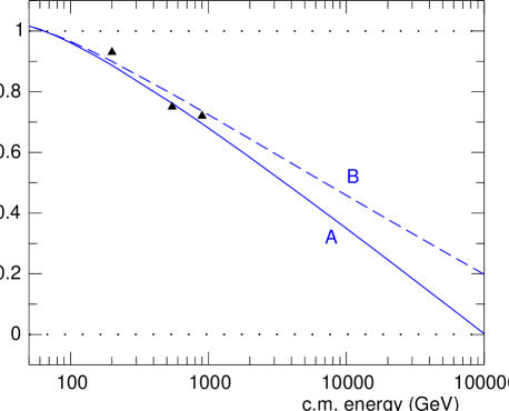
Figure 32: Energy dependence of the superposition parameter $\alpha$ (fraction of soft events) in the two cases of a linear (solid line, Eq. (153)) and quadratic (dashed line, Eq. (154)) dependence of the average multiplicity of the semi-hard component on c.m. energy. The triangles are the result of the UA5 analysis [93].

The success of the phenomenological analysis in terms of NB (Pascal) MD’s of experimental data or available fits on collective variable properties, together with the QCD roots of the MD’s itself, suggest to consider these results as a sound basis for the description of possible multiparticle production scenarios in the TeV energy domain accessible to future experiments at CERN LHC. The approach we decided to follow depends in a crucial way on the NB (Pascal) MD parameters behaviour and the problem one would like to solve first is how to extrapolate these parameters ($\bar{n}_{i}$ and $k_{i}$ ($i=$ soft, semi-hard)) from the GeV to the TeV energy region [93, 94].

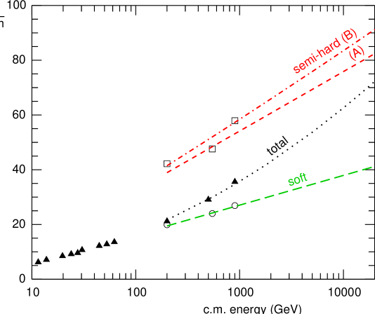
Figure 33: Average multiplicity $\bar{n}$ vs. c.m. energy. The figures shows experimental data (filled triangles) from ISR and SPS colliders, the UA5 analysis with two NB (Pascal) MD’s of SPS data (circles: soft component; squares: semi-hard component), together with our extrapolations (lines: dotted: total distribution; dashed: soft component; short-dashed: semi-hard component, Eq. (153); dot-dashed: semi-hard component, Eq. (154) [93].

4.7.1 The average charged multiplicities.

Extrapolations from UA5 collaboration results on soft events suggest

$$\bar{n}_{\text{soft}}(\sqrt{s})=-5.54+4.72\ln\sqrt{s},$$ (152)

and estimates for semi-hard events from UA1 collaboration [91] give

$$\bar{n}_{\text{semi-hard}}(\sqrt{s})\approx 2\bar{n}_{\text{soft}}(\sqrt{s})\qquad\text{(case A)}$$ (153)

or

$$\bar{n}_{\text{semi-hard}}(\sqrt{s})=2\bar{n}_{\text{soft}}(\sqrt{s})+0.1\ln^{2}\sqrt{s}\qquad\text{(case B)}.$$ (154)

Since the average charged multiplicity is well parametrised by $\bar{n}_{\text{total}}(\sqrt{s})=3.01-0.474\ln\sqrt{s}+0.75\ln^{2}\sqrt{s}$ and the total charged average multiplicity $\bar{n}_{\text{total}}$ in terms of the superposition of two components with weight $\alpha$ turns out to be

$$\bar{n}_{\text{total}}(\sqrt{s})=\alpha\bar{n}_{\text{soft}}+(1-\alpha)\bar{n}_{\text{semi-hard}},$$ (155)

it follows that

$$\alpha_{0}=2-\bar{n}_{\text{total}}/\bar{n}_{\text{soft}}$$ (156)

in the case (A) and

$$\alpha=1+(\bar{n}_{\text{soft}}-\bar{n}_{\text{total}})/(\bar{n}_{\text{soft}}-0.1\ln^{2}\sqrt{s})$$ (157)

in the case (B). We expect therefore for cases (A) and (B) in the TeV region the general trends of $\alpha$ and the average charged multiplicities shown in Figures 32 and 33.

$\bar{N}$                                                         ${\bar{n}_{c}}$

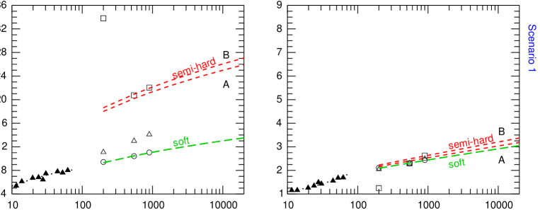
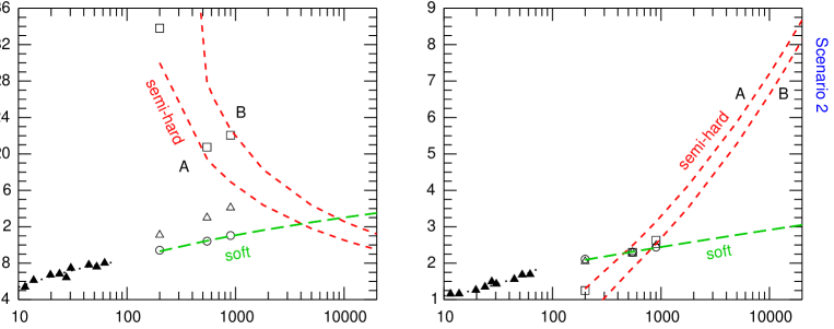
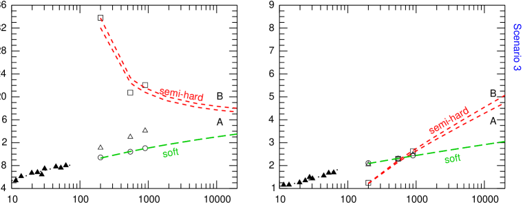
Figure 34: Clan parameters $\bar{N}$ (panels in the left columns) and ${\bar{n}_{c}}$ (panels in the right column) are plotted for the scenarios described in the text (from top to bottom: first row: scenario 1; second row: scenario 2; third row: scenario 3). The figures shows experimental data (filled triangles) from ISR and SPS colliders, the UA5 analysis with two NB(Pascal) MD’s of SPS data (circles: soft component; squares: semi-hard component), together with our extrapolations (lines: dotted: total distribution; dashed: soft component; short-dashed: semi-hard component) [93].

4.7.2 The $k$ and $k_{i}$ ($i$=soft, semi-hard) parameters.

For the soft component it is not too daring to assume that KNO scaling is not violated in the new energy domain, and accordingly to decide that $D^{2}_{\text{soft}}/\bar{n}^{2}{{}_{\text{soft}}}$ remains approximately constant ($\approx 0.143$) with $k_{\text{soft}}$ above 200 GeV c.m.  energy $\approx 7$. Assumptions for the semi-hard component are more delicate and at least three possibilities which could characterise different scenarios should be examined.

In scenario 1, being $k_{\text{semi-hard}}$ in Fuglesang’s fit [42] approximately 13 at 900 GeV and $\bar{n}_{\text{semi-hard}}$ even larger than $\bar{n}_{\text{soft}}$ it is assumed that $k_{\text{semi-hard}}$ remains approximately constant with $D^{2}_{\text{semi-hard}}/\bar{n}^{2}{{}_{\text{semi-hard}}}\approx 0.09$, i.e., in this scenario KNO scaling is not violated in the two separate components contributing to the total sample of events.

In scenario 2, a strong KNO violation is assumed with $D^{2}_{\text{semi-hard}}/\bar{n}^{2}_{\text{semi-hard}}$ growing logarithmically with c.m. energy above 200 GeV and $k_{\text{semi-hard}}$ falling from 79 at 200 GeV to $\approx 3$ at 14 TeV ($k_{\text{semi-hard}}\approx{1/\ln\sqrt{s}}$).

Scenario 3 is the QCD-inspired one, i.e.,

$$k_{\text{semi-hard}}^{-1}=a+b\sqrt{\alpha_{\text{strong}}}$$ (158)

with $\alpha_{\text{strong}}\approx(\ln Q/Q_{s})^{-1}$, $Q$ and $Q_{s}$ are respectively the initial virtuality and the cut-off of the parton shower. $Q_{s}$, $a$ and $b$ are determined by a least square fit to the values of $k_{\text{semi-hard}}$ given by UA5 collaboration at 200 GeV, 546 GeV and 900 GeV. It follows

$$k_{\text{semi-hard}}^{-1}=0.38-\sqrt{\frac{0.42}{{\ln(\sqrt{s}/10)}}}$$ (159)

The decrease of $k_{\text{semi-hard}}$ is milder than in scenario 2, it goes from 13 at 200 GeV to 7 at 14 TeV; interestingly, the QCD inspired behaviour of $k_{\text{semi-hard}}$ is intermediate among the previous two, with no KNO scaling and strong KNO scaling violation respectively, which describe probably quite extreme situations.

4.7.3 Clan structure analysis of $pp$ collisions in the TeV region

Following the above general discussion on the possible behaviours of NB (Pascal) MD’s parameters in the TeV region, their interpretation in terms of the average number of clans, $\bar{N}$, and of the average number of particles per clan, ${\bar{n}_{c}}$, reveals unsuspected new features which deserve particular attention (See Figure 34).

Of course, in scenario 1, $\bar{N}_{\text{soft}}$ and $\bar{N}_{\text{semi-hard}}$ are expected to continue to increase —although $k_{\text{soft}}$ and $k_{\text{semi-hard}}$ remain constant— in view of the increase of the average charged multiplicity in each component. Clans are quite numerous but their size (i.e., $\bar{n}_{c,\text{soft}}$ and $\bar{n}_{c,\text{semi-hard}}$) although still growing with c.m. energy remains quite small. Notice that the behaviour of clans of the soft component is the same by assumption in all scenarios. The situation is similar to what we know from the GeV region. What makes this analysis striking is the remark that $\bar{N}_{\text{semi-hard}}$ in the 2nd and 3rd scenarios becomes smaller with the increase of the c.m. energy, and the average number of particles per clan very large. The phenomenon is enhanced in particular in scenario 2 where $D^{2}_{\text{semi-hard}}/\bar{n}^{2}{{}_{\text{semi-hard}}}$ shows a dramatic increase with energy as requested by strong KNO scaling violation. The reduction of $\bar{N}_{\text{semi-hard}}$ and the simultaneous quick increase of $\bar{n}_{\text{semi-hard}}$ suggests that in the scenarios 2 and 3 the available c.m. energy goes more in particle production within a clan rather than in new clan production, differently from what was found in scenario 1.

Figure 35: E735 results on charged particle multiplicity distributions in $pp$ collisions at various energies in full phase-space compared with UA5 results at similar energies. Data from the two experiments which were taken at nearly the same energy are rescaled by the same factor [95].

Data on MD’s at 1.8 TeV c.m. energy (from E735 experiment [95]), when compared with our predictions are closer to scenario 2 but with an even wider MD. It is to be stressed that E735 results on full phase-space multiplicity distributions do not completely agree with those obtained at comparable energies at the S$p\bar{p}$S collider by the UA5 Collaboration [78, 27], see Fig. 35. Tevatron data are more precise than S$p\bar{p}$S data at larger multiplicities (they have larger statistics and extend to larger multiplicities than UA5 data), but much less precise at low multiplicity. Both sets of data show a shoulder structure, but the Tevatron MD is somewhat wider. It should be noticed that E735 data are measured only in $|\eta|<3.25$ and $p\kern-0.2pt\lower 4.0pt\hbox{\tiny T}>0.2$ GeV/$c$ then extended to full phase-space via a Monte Carlo program. Notwithstanding the mentioned discrepancy, there is consensus in accepting the presence of (at least) two substructures in the data, either related to the varying impact parameter [96] or to multiple parton scattering [97, 98]. In terms of the scenarios discussed in this Section, one can reasonably argue that scenario 1 is the less probable to occur and that therefore the above mentioned finding on clan reduction in scenarios 2 and 3 raises some interesting questions on the properties of clans themselves, i.e., how far the number of clans of the semi-hard component could be reduced in our framework? is the reduction to one or very few clans compatible with the structure of the semi-hard component? should we expect, with the increase of the c.m. energy of the collision, the onset of a new component to be added to the previous two? The attempt to answer these questions is postponed to the next sections, where also we would like to address the related question on the real nature of clans, which seems quite natural at this stage of our search, i.e., are clans observable (massive) objects?

4.7.4 Analysis in pseudo-rapidity intervals

We would like to point out that our study on the possible three scenarios in the TeV region based on extrapolations of the experimental knowledge of the GeV energy domain can be extended from full phase-space to rapidity intervals.

Since only after the classification of events (soft and semi-hard) has been carried out do we look at phase-space intervals, it seems quite reasonable to assume that the weight factor $\alpha$ depends on the c.m. energy (as in full phase-space) and not on the pseudo-rapidity interval $\eta_{c}$.

The $\eta_{c}$ dependence comes therefore from $\bar{n}_{i}$ and $k_{i}$ parameters only.

Table 2: Values of $1/k_{\text{total}}$, $1/k_{\text{soft}}$ and $1/k_{\text{semi-hard}}$ in our extrapolations for different rapidity intervals and for full phase-space (FPS). $1/k_{\text{soft}}$ and, in scenario 1, $1/k_{\text{semi-hard}}$, are energy independent and their value is given in the table; in the other cases we give the parameters and the form of the energy dependence [94].

interval	soft comp.	scenario 1	scenario 2	scenario 3
$|\eta|\leq\eta_{c}$	$k_{\text{soft}}^{-1}$	$k_{\text{semi-hard}}^{-1}$	$k_{\text{total}}^{-1}(\eta_{c},\sqrt{s})=$	$k_{\text{semi-hard}}^{-1}(\eta_{c},\sqrt{s})=$
			$a+b\ln\sqrt{s}$	$C+D/{\sqrt{\ln(\sqrt{s}/10)}}$
$\eta_{c}=1$	0.294	0.217	$a=0.02$ $b=0.08$	$C=0.97$ $D=-1.6$
$\eta_{c}=2$	0.286	0.172	$a=-0.06$ $b=0.08$	$C=0.88$ $D=-1.5$
$\eta_{c}=3$	0.250	0.156	$a=-0.12$ $b=0.08$	$C=0.72$ $D=-1.2$
FPS	0.143	0.077	$a=-0.082$ $b=0.0512$	$C=0.38$ $D=-0.65$

In order to be consistent with our assumptions in full phase-space, the single particle density must show an energy independent plateau which extends in pseudo-rapidity for some units around $\eta=0$ in each direction. Accordingly, the height of the plateau ($\bar{n}_{0}$) of the soft and semi-hard component is fixed equal to

$$\bar{n}_{0,\text{soft}}\approx 2.45$$ (160)

(a value compatible with low energy data [80] where only the soft component is present) and

$$\bar{n}_{0,\text{semi-hard}}\approx 6.4$$ (161)

(notice that the assumption of an energy independent plateau for the semi-hard component is not compelling and that the following increase with c.m. energy of $\bar{n}_{0,\text{semi-hard}}$ is again compatible with all our previous discussion: $\bar{n}_{0,\text{semi-hard}}\approx 6.3+0.07\ln\sqrt{s}$).

Finally

$$\bar{n}_{i}(\eta_{c})=2\bar{n}_{0,i}\eta_{c}(i=\text{soft},\text{semi-hard})$$ (162)

and

$$\bar{n}_{\text{total}}(\eta_{c},\sqrt{s})=\alpha_{\text{soft}}(\sqrt{s})\bar{n}_{\text{soft}}(\eta_{c})+[1-\alpha_{\text{soft}}(\sqrt{s})]\bar{n}_{\text{semi-hard}}(\eta_{c}).$$ (163)

Figure 36: The average number of clans, $\bar{N}$, (top two rows) and the average number of particles per clan, ${\bar{n}_{c}}$, (bottom two rows) are plotted against the c.m. energy for three rapidity intervals (dotted line: $\eta_{c}=1$; dash-dotted line: $\eta_{c}=2$; dashed line: $\eta_{c}=3$) and for f.p.s. (solid line), for each scenario (in columns, from left to right: scenario 1, 2 and 3) and for each component (in rows, from top to bottom: soft and semi-hard) [94].

By recalling that

$$\bar{n}^{2}_{\text{total}}(\eta_{c},\sqrt{s})\left(1+\frac{1}{k_{\text{total}}(\eta_{c},\sqrt{s})}\right)=\alpha(\sqrt{s})\bar{n}^{2}_{\text{soft}}(\eta_{c},\sqrt{s})\left(1+\frac{1}{k_{\text{soft}}(\eta_{c},\sqrt{s})}\right)\\ +(1-\alpha(\sqrt{s}))\bar{n}^{2}_{\text{semi-hard}}(\eta_{c},\sqrt{s})\left(1+\frac{1}{k_{\text{semi-hard}}(\eta_{c},\sqrt{s})}\right)$$ (164)

results contained in table 2 are obtained. Clan structure analysis confirms the general trends found in full phase-space, favouring a lower number of clans of smaller size in more restricted rapidity intervals; of particular interest is again the semi-hard component. The results are illustrated in Fig. 36. In scenario 1, as the energy increases one notices a copious production of clans of nearly equal size in all rapidity intervals. In scenario 2, in all pseudo-rapidity intervals, to the higher aggregation of newly created particles into existing clans it follows the aggregation of clans into super-clans favouring stronger long range correlations. Scenario 3 (the QCD-inspired one) leads to predictions which are —as usual— intermediate between the previous two.

4.8 Hints from CDF

At the Tevatron, the subsample of events with no energy clusters above 1.1 GeV and the subsample of remaining events were separated in the total sample of $p\bar{p}$ events collected in the pseudo-rapidity window $|\eta|<1$ with CDF minimum bias trigger at $\sqrt{s}=630$ GeV and at $\sqrt{s}=1800$ GeV [99].

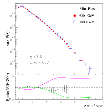
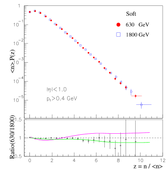
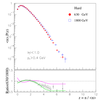
Figure 37: Multiplicity distributions for the full minimum bias, the ‘soft’ and the ‘hard’ samples at 1800 and 630 GeV from CDF; data are plotted in KNO variables. In the bottom panel of each figure the ratio of the two above distributions is shown. The two continuous lines delimit the band of all systematic uncertainties [99].

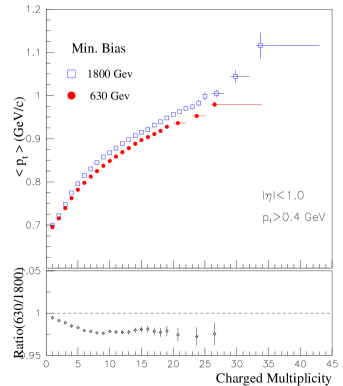
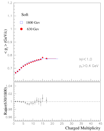
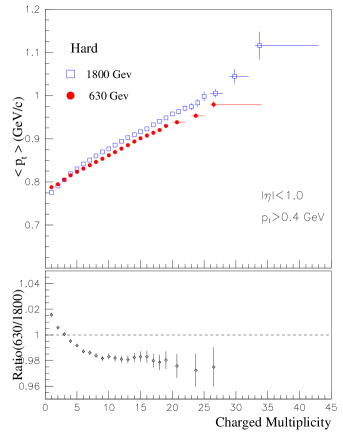
Figure 38: Mean transverse momentum vs multiplicity for the full minimum bias, the ‘soft’ and the ‘hard’ samples at 1800 and 630 GeV from CDF. On the bottom panel of each figure the ratio of the two curves is shown [99].

Being the two samples of events highly enriched in soft and hard interactions respectively and the Collaboration quite aware of the difficulty of a correct identification and separation of jets with transverse energy lower than 5 GeV, events with no clusters were called ‘soft’ and those with at least one cluster, ‘hard’. $n$ charged particle multiplicity distributions for the minimum bias samples at the two energies were plotted in the KNO form and showed, in the interval $|\eta|<1$, KNO scaling violations. When the two samples of events are separately plotted the soft component satisfies KNO scaling, whereas the hard component clearly violates KNO scaling, suggesting that the behaviour of the second component is the main cause of KNO scaling violations in the full sample, as shown in Fig. 37.

Interestingly the mean transverse momentum $\langle p_{T}\rangle$ when plotted versus $n$ charged multiplicity for the full minimum bias sample is larger at 1800 GeV than at 630 GeV, whereas it does not grow with the c.m. energy in the soft sample (See Fig. 38.) The different behaviour at the two energies in the full minimum bias sample is therefore entirely due to the hard sample and it is probably the effect of high transverse energy interactions (mini-jets in the literature).

These results, although limited to a single pseudo-rapidity interval only, provide an interesting experimental support to the two main assumptions which justified our approach to the TeV energy domain in $pp$ collisions, i.e.:

a. that there are at least two components in the total sample of events at threshold of the TeV energy domain (they are called ‘soft’ and ‘semi-hard’ in Ref. [42] and by us (Sections 4.5 and 4.7), and ‘soft’ and ‘hard’ in the paper by the CDF Collaboration);

b. that the soft component satisfies KNO scaling.

In addition, as far as the second component (the semi-hard one) is concerned, the scenario with strong KNO scaling violation or the one based on QCD inspired behaviour seem favoured with respect to the scenario with KNO scaling.

4.9 Forward-backward multiplicity correlations. The demand for the existence of clans.

The experimental problem consists in studying, in each event, the number of particles falling in the forward hemisphere (F) and in the backward hemisphere (B) [33]. Usually, the average number of particles in the B hemisphere, $\bar{n}_{B}$, is successfully parametrised in terms of the number of particles in the F hemisphere, $n_{F}$, according to the following linear relation:

$$\bar{n}_{B}(n_{F})=a+b_{\text{FB}}n_{F},$$ (165)

where $b_{\text{FB}}$ is the FB multiplicity correlation strength:

$$\begin{split}b_{\text{FB}}&\equiv\frac{\text{Cov}[n_{F},n_{B}]}{(\text{Var}[n_{F}]\text{Var}[n_{B}])^{1/2}}\\ &=\frac{\langle(n_{F}-\bar{n}_{F})(n_{B}-\bar{n}_{B})\rangle}{\left[\langle(n_{F}-\bar{n}_{F})^{2}\rangle\langle(n_{B}-\bar{n}_{B})^{2}\rangle\right]^{1/2}}.\end{split}$$ (166)

The existence of strong correlations between particles in the two hemispheres is an important effect and could be a signal of large colour exchange among partons at parton level. It is instructive with this aim to examine the experimental situation on FB multiplicity correlations in $pp$ collisions and $e^{+}e^{-}$  annihilation.

In $pp$ collisions the F hemisphere coincides with the region of the outgoing proton, the B hemisphere is the symmetric region in the opposite direction. In $pp$ collisions, $b_{\text{FB}}$ is growing with c.m. energy and is rather large. At 63 GeV (ISR) $b_{\text{FB}}=0.156\pm 0.013$ and at 546 GeV (UA5) $b_{\text{FB}}=0.43\pm 0.01$ in $1<|\eta|<4$ and $b_{\text{FB}}=0.58\pm 0.01$ in $0<|\eta|<4$. Its general trend with c.m. energy is given by

$$b_{\text{FB}}=-0.019+0.061\ln s$$ (167)

In $e^{+}e^{-}$  annihilation the F hemisphere is chosen randomly between the two hemispheres defined by the plane perpendicular to the thrust axis. OPAL collaboration has found $b_{\text{FB}}=0.103\pm 0.007$ for the total sample of events and $b_{\text{FB}}\approx 0$ in the separate two- and three-jets sample of events. TASSO Collaboration finds $b_{\text{FB}}=0.080\pm 0.016$ in the total sample of events, we do not have estimates in this case of $b_{\text{FB}}$ in the separate samples of events. In conclusion in $e^{+}e^{-}$  annihilation $b_{\text{FB}}$ grows with energy but is rather small.

Accordingly our interest on the theory side was limited to symmetric reactions only [33], although a generalisation to asymmetric collisions can be worked out [100].

The number of F and B particles, $n_{F}$ and $n_{B}$, are of course random variables with $n_{F}+n_{B}=n$ and

$$P_{n}=\sum_{n=n_{F}+n_{B}}P_{\text{total}}(n_{F},n_{B}).$$ (168)

$P_{\text{total}}(n_{F},n_{B})$ is the joint distribution for the weighted superposition of different classes of events and is equal to $\alpha P_{1}(n_{F},n_{B})+(1-\alpha)P_{2}(n_{F},n_{B})$; $\alpha$ is the weight of class 1 of events with respect to the total sample of events. The calculation of $b_{\text{FB}}$ according to Eq. (166) leads then to the following result:

$$b_{\text{FB}}=\frac{\alpha b_{1}{D^{2}_{n,1}}/(1+b_{1})+(1-\alpha)b_{2}{D^{2}_{n,2}}/(1+b_{2})+\frac{1}{2}\alpha(1-\alpha)(\bar{n}_{2}-\bar{n}_{1})^{2}}{\alpha{D^{2}_{n,1}}/(1+b_{1})+(1-\alpha){D^{2}_{n,2}}/(1+b_{2})+\frac{1}{2}\alpha(1-\alpha)(\bar{n}_{2}-\bar{n}_{1})^{2}}.$$ (169)

Here $b_{1}$ and $b_{2}$ are the correlation strengths of events of class 1 and 2, $D_{1}$ and $D_{2}$ the corresponding dispersions and $\bar{n}_{1}$ and $\bar{n}_{2}$ the corresponding average multiplicities.

For $b_{1}=b_{2}=0$, one has $b_{\text{FB}}\to b_{12}$ and the previous formula is reduced to the following one

$$b_{12}=\frac{\frac{1}{2}\alpha(1-\alpha)(\bar{n}_{2}-\bar{n}_{1})^{2}}{\alpha{D^{2}_{n,1}}+(1-\alpha){D^{2}_{n,2}}+\frac{1}{2}\alpha(1-\alpha)(\bar{n}_{2}-\bar{n}_{1})^{2}}.$$ (170)

It is a general property of the two formulae to be independent of the specific form of the $n_{1}$ particles and $n_{2}$ particles multiplicity distributions, $P_{n_{1}}$ and $P_{n_{2}}$, and to depend on $\alpha$, $\bar{n}_{1}$, $\bar{n}_{2}$, $D_{1}$ and $D_{2}$ parameters only.

OPAL collaboration measured FB multiplicity correlation strengths in $e^{+}e^{-}$  annihilation in the two separate samples of events (2-jet sample and 3-jet sample) and in the total sample [89]. It has been found that $b_{1}\approx b_{2}\approx 0$ and $b_{\text{FB}}=b_{12}=0.103\pm 0.007$ respectively. Being $\alpha=0.463$, $\bar{n}_{1}=18.4$, $D_{1}^{2}=25.6$, $\bar{n}_{2}=24.0$ and $D_{2}^{2}=44.6$, the theoretical estimate of $b_{12}$ according to formula (170) turns out to be 0.101 in perfect agreement with the experimental value $0.103\pm 0.007$. The success of our formula (170) in describing FB multiplicity correlations in $e^{+}e^{-}$  annihilation should be contrasted with its failure in describing $b_{\text{FB}}$ in $pp$ collisions: $b_{1}$ and $b_{2}$ are expected to be different from zero in the latter case and the more general formula (169) is needed. The parameters of such general formula can be computed under the assumptions that :

a) particles are independently produced;

b) they are binomially distributed in the F and B hemispheres;

c) the overall MD for each component (soft and semi-hard) is a NB (Pascal) MD with characteristic parameters $\bar{n}_{i}$ and $k_{i}$ ($i=1,2$).

It can then be concluded that charged particles FB multiplicity correlations are not compatible with independent particles emission and that charged particles FB multiplicity correlations are compatible with the production of particles in clusters (i.e., clans in view of assumption c). It follows that:

a. the joint probability distribution $P(n_{F},n_{B})$ is written as the convolution over the number of produced clans and over the partitions of forward and backward produced particles among clans;

b. the symmetry argument should be used;

c. the introduction of a leakage parameter $p$ is needed: the new parameter $p$ controls the probability that a binomially distributed particle (and generated by one clan lying in one hemisphere) has to leak in the opposite hemisphere ($p=1$ means no leakage, the variation domain of $p$ is $1/2<p<1$ and $p<0.5$ implies that the clan to which the emitted particle is belonging is classified in the wrong hemisphere);

d. a covariance parameter, $\gamma$, between F and B particles within a clan is also introduced;

e. within this framework clans are binomially produced in the F and B hemispheres with the same probabilities and particles belonging to a clan are independently produced in the two hemispheres.

From these assumptions one gets that:

i. clan structure analysis is applicable for each component,

ii. clans in each component are independently emitted (their distribution is Poissonian),

iii. clans are binomially distributed in the two hemispheres,

iv. logarithmically produced particles from each clan are also binomially distributed in the F and B hemispheres but with different probabilities (the corresponding leakage parameters are different).

The parameters of formula (169) can then be calculated. We find indeed for the single component strength

$$\begin{split}b_{\text{FB}}^{(i)}&=\frac{D^{2}_{N}-4\langle d^{2}_{N_{F}}(N)\rangle(p-q)^{2}+4\bar{N}\gamma/{\bar{n}_{c}}^{2}}{D^{2}_{N}+4\langle d^{2}_{N_{F}}(N)\rangle(p-q)^{2}-4\bar{N}\gamma/{\bar{n}_{c}}^{2}+2\bar{N}D^{2}_{c}/{\bar{n}_{c}}^{2}}\\ &=\frac{D^{2}_{n}/\bar{n}-D^{2}_{c}/{\bar{n}_{c}}-4\langle d^{2}_{N_{F}}(N)\rangle(p-q)^{2}{\bar{n}_{c}}/\bar{N}+4\gamma/{\bar{n}_{c}}}{D^{2}_{n}/\bar{n}+D^{2}_{c}/{\bar{n}_{c}}+4\langle d^{2}_{N_{F}}(N)\rangle(p-q)^{2}{\bar{n}_{c}}/\bar{N}-4\gamma/{\bar{n}_{c}}}.\end{split}$$ (171)

Formula (171) is valid for the class of CPMD’s. Assuming in addition, according to iv, that clans in each component are of NB (Pascal) MD type with $k_{i}$ and $\bar{n}_{i}$ parameters, one has

$$\begin{split}b_{\text{FB}}^{(i)}&=2\bar{n}_{i}p_{i}(1-p_{i})/(\bar{n}_{i}+k_{i}-2\bar{n}_{i}p_{i}(1-p_{i}))\\ &=2\beta_{i}p_{i}(1-p_{i})/(1-2\beta_{i}p_{i}(1-p_{i})),\end{split}$$ (172)

with $\beta_{i}=\bar{n}_{i}/(\bar{n}_{i}+k_{i})$. It should be remembered that the leakage parameter $p_{i}$ is the fraction of particles within one clan which fall in the same hemisphere where the clan was produced. Assuming that the semi-hard component is negligible at $\sqrt{s}=63$ GeV and knowing $b_{\text{FB}}(\sqrt{s}=63~{}\text{GeV})=0.156\pm 0.013$ from experiments, and of course $\bar{n}_{\text{soft}}$, $k_{\text{soft}}$ leakage parameter for the soft component can be determined. We find $p_{\text{soft}}=0.78$, i.e., 22% of the particles are expected to leak from clans in one hemisphere to the opposite one.

Figure 39: Predictions for the correlation coefficients for each component (soft and semi-hard) and for the total distribution in $p\bar{p}$ collisions. For each scenario, three cases are illustrated, corresponding to the three numbered branches: leakage increasing with $\sqrt{s}$ (upper branch, ), constant leakage (middle branch, ) and leakage decreasing with $\sqrt{s}$ (lower branch, ). Leakage for the soft component is assumed constant at all energies. The dotted line is a fit —see Eq. (167)— to experimental values [33].

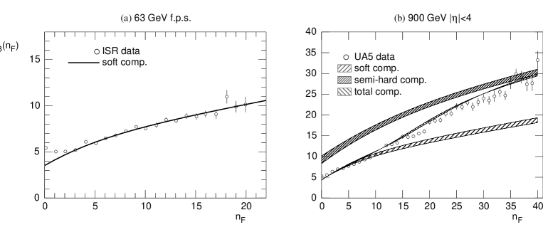
Figure 40: Results of the weighted superposition model for $\bar{n}_{B}(n_{F})$ vs. $n_{F}$ compared to experimental data in full phase-space at 63 GeV (a) and in the pseudo-rapidity interval $|\eta|<4$ at 900 GeV (b) [33].

The relatively small increase of the average number of particles per clan from 63 GeV to 900 GeV for the soft component (${\bar{n}_{c}}$ goes from $\approx 2$ to $\approx 2.44$) suggests to consider $p_{\text{soft}}$ constant throughout the GeV energy region. Accordingly, being $\bar{n}_{\text{soft}}$ and $k_{\text{soft}}$ known at 546 GeV, $b_{\text{FB},\text{soft}}$ for the soft component can be determined at such energy; its value, inserted in Eq. (169), allows the determination of $b_{\text{FB},\text{semi-hard}}$ in view of the fact that $b_{\text{FB},\text{total}}=0.58$. It is found that $p_{\text{semi-hard}}$($\sqrt{s}=546$ GeV) = 0.77. The relatively small increase of the average number of particles per clan also for the semi-hard component, from 200 GeV up to 900 GeV (${\bar{n}_{c}}$ goes from 1.64 to 2.63), suggests to take also $p_{\text{semi-hard}}$ constant in the GeV region.

Under the just mentioned assumptions:

a) the correlation strength c.m. energy dependence is correctly reproduced in the GeV energy range from ISR up UA5 top c.m. energy and follows the phenomenological formula $b_{\text{FB}}=-0.019+0.061\ln s$ (Figure 39).

b) $\bar{n}_{B}(n_{F})$ vs $n_{F}$ behaviour at 63 GeV c.m. energy (ISR data) is quite well reproduced in terms of the soft component (a single NB (Pascal) MD) only and at 900 GeV c.m. energy (UA5 data) in terms of the weighted superposition of soft and semi-hard components, i.e., of the superposition of two NB (Pascal) MD’s. (Figure 40).

Concerning the general trends of $b_{\text{FB}}$ vs $\sqrt{s}$ and of $\bar{n}_{B}(n_{F})$ vs $n_{F}$ in the TeV energy domain, the situation is not unanimous. In some approaches one expects a continuous increase towards the value 1: either reasoning on the use of a soft and a hard component within the eikonal model for mini-jets production [101] or (in a purely statistical analysis) on the independent production of pairs of particles [102], rather than of individual particles or clusters/clans. The three scenarios extrapolated from our knowledge on $pp$ collisions in the GeV region and discussed in Section 4.7, provide different predictions. Being for instance in all scenarios at 14 TeV $\bar{n}_{c,\text{soft}}\approx 2.98$ ($\bar{n}_{c,\text{soft}}$ is $\approx 2$ at 63 GeV and $\approx 2.63$ at 900 GeV) to assume $p_{\text{soft}}$ constant ($\approx 0.78$) also in the new energy domain seems quite reasonable. The situation for $p_{\text{semi-hard}}$ is different. With the exception of the first scenario for which the validity of KNO scaling is assumed also for the semi-hard component and $\bar{n}_{c,\text{semi-hard}}$ goes from $\approx 2.63$ at 900 GeV to $\approx 3.28$ at 14 TeV after a very weak increase in the GeV energy region, $p_{\text{semi-hard}}$ constant is an unrealistic assumption; $\bar{n}_{c,\text{semi-hard}}$ in the second scenario where strong KNO scaling violation is allowed is indeed $\approx 2.63$ at 900 GeV but $\approx 7.96$ at 14 TeV and in the third scenario (the QCD inspired one) the $\bar{n}_{c,\text{semi-hard}}$ values at the two energies are $\approx 2.5$ and $\approx 5$ at the two energies.

What should be noticed is that in all above mentioned scenarios $b_{\text{FB}}$ is bending in the new region and that $b_{\text{FB}}$ bending is more pronounced if $p_{\text{semi-hard}}$ increases (less particle leakage from clans) and it is less pronounced when $p_{\text{semi-hard}}$ decreases (more particle leakage from clans). $b_{\text{FB},\text{total}}$ bending can be therefore reduced by allowing more particle leakage from individual clans, i.e., by allowing a larger particle flow from one hemisphere to the opposite one. The real question is how far in energy the empirical fit on $b_{\text{FB},\text{total}}$ c.m. energy dependence will continue to find experimental support without spoiling the main assumptions of our approach to FBMD correlations.

Figure 41: Energy dependence of the correlation coefficients for each component (soft and semi-hard) and for the total distribution in $p\bar{p}$ collisions. The dotted line is a fit —see Eq. (167)— to experimental values [103].

It is indeed instructive to reexamine the three scenarios extrapolated in the TeV energy domain in order to include in our scheme the $b_{\text{FB},\text{total}}$ points at 1000 GeV and 1800 GeV measured by E735 Collaboration at Fermilab to sit on the same straight line in Figure 41 of the other points at lower c.m. energies. It is remarkable that the inclusion of the new points demands that $p_{\text{semi-hard}}$ must decrease and accordingly particle leakage from one hemisphere to the opposite one must increase in all scenarios.

Satisfactory results for $b_{\text{FB},\text{total}}$ energy dependence are obtained in all three scenarios in Figure 41 by taking $p_{\text{soft}}\approx 0.8$ and $p_{\text{semi-hard}}\approx 0.84-0.07\ln(\sqrt{s}/200)$ for $\sqrt{s}\geq 200$ GeV.

It should be pointed out that in the scenario characterised by a semi-hard component with strong KNO scaling violation (scenario 2) FBMC strength has a less steep behaviour with the increase of the c.m. energy of the collision and its saturation towards 1 —as that of $b_{\text{FB},\text{total}}$— is quicker than in the other scenarios. It turns out that the linear behaviour of $b_{\text{FB},\text{total}}$ with the increase of c.m. energy shown in Figure 41 is incompatible with our approach to FBMD correlations above 2.5 TeV in scenario 1, above 3.5 TeV in scenario 2 and above 5 TeV in scenario 3. By incompatible we mean that leakage parameter $p_{\text{semi-hard}}$ cannot be adjusted in order to reproduce the eventual linear behaviour of $b_{\text{FB},\text{total}}$ above the mentioned c.m. energy extreme values in the different scenarios without spoiling the model itself.

On the contrary the experimental finding of the mentioned linear fit of $b_{\text{FB},\text{total}}$ at higher c.m. energy, say at LHC, would demand in our approach the existence of a third class of events to be added to the soft and semi-hard ones with even larger leakage of particles from clans in one hemisphere to the opposite one than that given by the a logarithmic decrease with c.m. energy of $p_{\text{semi-hard}}$.

It seems that in the new class clan production is therefore disfavoured with respect to the production of more particles within clans. The main characteristic of such events is to be composed of few high particles density clans generated by necessarily high virtuality ancestors. This fact if confirmed would have an interesting counterpart at parton level and allow a suggestive interpretation of the completely different behaviour of the FB multiplicity correlations in $pp$ collisions and $e^{+}e^{-}$  annihilation.

As already seen, in $e^{+}e^{-}$  annihilation, FB multiplicity correlations are almost inexistent in the two component and very weak in the total sample of events (an effect entirely due to the superposition of the two classes of events). Here clans are numerous but quite small in size, i.e., the independent intermediate gluon sources (the BGJ’s) —the clan ancestors at parton level— are expected to be generated quite late in the production process at relatively low virtualities, implying small colour exchange among partons and then very weak FB multiplicity correlations among hadrons.

In $pp$ collisions clans are less numerous than in $e^{+}e^{-}$  annihilation but their size is larger, i.e., more particles are contained within each clan. At parton level one should expect that BGJ’s are generated quite early in the production process at relatively high virtualities with enough room for many parton splittings and consequently stronger colour exchanges. All that at hadron level will lead to quite remarkable FBMC’s. In this framework the eventual third class of events whose existence would be determined by the observation of a linear increase of $b_{\text{FB},\text{total}}$ with c.m. energy in the proper TeV energy domain will have some peculiar characteristics, which make its finding particularly appealing. First of all one should see in these events a reduction of the average number of clans to few units in order to guarantee a high particle population per clan and a quite consistent particle leakage from one hemisphere to the opposite one. At parton level the fewer BGJ’s production of the new class of events with respect to the semi-hard one should be originated by a very high virtuality process —much higher than for semi-hard events— leading to high parton density regions characterised by huge colour exchanges.

Figure 42: $\langle z^{2}\rangle_{n}$ vs $n$ at 900 GeV in the interval $1<|\eta|<4$. Data points are from UA5 Collaboration, the solid line is the result of our model in $0<|\eta|<4$, the dash-dotted line is a linear fit [103].

Another variable sometime used in the literature in addition to $b_{\text{FB}}$ should be mentioned: it is the average of the forward backward particle multiplicity difference over all events at fixed multiplicity $n$, i.e., $\langle z^{2}\rangle_{n}=\langle n_{F}-n_{B}\rangle_{n}$. The new variable works at a deeper level of investigation than $b_{\text{FB}}$ (the latter is related to the average of $\langle n_{F}-n_{B}\rangle_{n}$ over all multiplicities) and it is of particular interest for global properties of the collisions related to average $n$. In our framework one has

$$\langle z^{2}\rangle_{n}=\frac{4d^{2}_{n_{F},\text{soft}}(n)\alpha P_{\text{soft}}(n)}{P_{\text{total}}(n)}+\frac{4d^{2}_{n_{F},\text{semi-hard}}(n)(1-\alpha)P_{\text{semi-hard}}(n)}{P_{\text{total}}(n)},$$ (173)

with $P_{\text{total}}(n)=\alpha P_{\text{soft}}(n)+(1-\alpha)P_{\text{semi-hard}}(n)$.

In Figure 42, data points from UA5 collaboration in $1<|\eta|<4$ at 900 GeV on $\langle z^{2}\rangle_{n}$ vs. $n$ are compared with our model results in full phase-space (solid line) as well as with the behaviour predicted in the model of Chou and Yang [104] (dashed line). The latter model supposes a composition of ‘stochastic’ (i.e., Poissonian) fluctuations in $z$ with ‘non-stochastic’ ones (in $n$, obeying KNO scaling), composition which is regulated by the collision geometry; in this scheme one obtains a linear dependence of $\langle z^{2}\rangle_{n}$ on $n$. Below $n\approx 40$, no differences between the two models are visible and both models are in agreement with experiments. Above $n\approx 40$, our model shows a clear ”hump” structure. The situation in such range is not experimentally clear and consequently no conclusions can be drawn on this point. Predictions on $\langle z^{2}\rangle_{n}$ vs.  $n$ behaviour in the possible scenarios expected in the TeV energy domain are discussed in reference [103]. The behaviour of the variable $\langle z^{2}\rangle_{n}$ has also been used as one possible evidence for a phase-transition [105].

4.10 Are clans massive objects?

The success of clan structure analysis in interpreting multiparticle production phenomenology raises, as pointed out at the end of section 4.7, many intriguing questions. Among them the problem of the clan mass is of particular interest. The first search on the subject goes back to A. Bialas and A. Szczerba [106]. The attempt is based on a generalisation of standard clan Poissonian production mechanism with two additional assumptions on clans distribution in rapidity variable and on the angular distribution of particle decay in a clan. Let us review briefly the main content of this search. Clans, Poissonianly distributed and independently emitted in bremsstrahlung-like fashion, are characterised using energy and (longitudinal) momentum conservation by the following single-clan (pseudo)-rapidity density

$$\frac{dN}{d\eta}=\lambda(1-x^{+})^{\lambda}(1-x^{-})^{\lambda},$$ (174)

with $x^{\pm}=(m_{T}/\sqrt{s})e^{\pm\eta}$.

Notice that $\lambda$ is the plateau height (the average number of clans per rapidity unit), $m_{T}$ the clan transverse mass ($m_{T}=\sqrt{m^{2}+p_{T}^{2}}$), $\eta$ is the clan (pseudo)-rapidity and $\sqrt{s}$ the c.m. energy (clan emission is limited to the interval $|\eta|<\ln(\sqrt{s}/m_{T})$. Furthermore particle probability density function inside a clan (assumed to be in $\eta_{0}$) on the hypothesis of isotropic decay is given by

$$\Phi(\eta,\eta_{0})=\left[2\omega\cosh^{2}\left(\frac{\eta-\eta_{0}}{\omega}\right)\right]^{-1},$$ (175)

where $\omega$ is a free parameter; distribution amplitude is proportional to $\omega$ and $\omega=1$ corresponds to an isotropic decay.

By assuming next that particles will be produced in each clan according to a logarithmic MD, whose generating function is given by $g_{\text{log}}(z)=\ln(1-z\beta)/\ln(1-\beta)=\sum_{n}P_{n}^{\text{(log)}}z^{n}$ and the average number of particles per clan by

$${\bar{n}_{c}}^{\text{(log)}}=\frac{\beta}{(\beta-1)\ln(1-\beta)},$$ (176)

with $\beta=\bar{n}/(\bar{n}+k)$, one finds that the generating function for the MD in the interval $\Delta\eta$ turns out to be

$$G(\lambda,\Delta\eta)=\exp\left\{\int\frac{dN}{d\eta}\frac{\ln\left[1-\frac{\beta}{1-\beta}p(\eta_{0};\Delta\eta)(z-1)\right]}{\ln(1-\beta)}d\eta_{0}\right\}$$ (177)

with

$$p(\eta_{0},\Delta\eta)=\int_{\Delta\eta}\Phi(\eta,\eta_{0})d\eta_{0}.$$ (178)

$p(\eta_{0},\Delta\eta)$ describes the fraction of particles generated by a clan with (pseudo)-rapidity $\eta_{0}$ falling in the interval $\Delta\eta$. It is assumed in addition that emitted particles by each clan are independently produced in rapidity. With a convenient choice of the parameters ($\lambda=0.855$, $m_{T}=3.15$ (GeV/c²), $\omega=1.45$, $\beta=0.90$) UA5 data at 546 GeV c.m. energy are approximately reproduced by the generating function of the model $G(z,\Delta\eta)$. The corresponding $n$ charged particle MD, $P_{n}$, is not a NB (Pascal) MD except in full phase-space and forward backward multiplicity correlations are not correctly reproduced by the model. These considerations notwithstanding, the above results are in our opinion quite instructive, although not satisfactory, in that they show a possible way to determine clan width and mass. Accordingly, we decided to extend the search on clan masses performed in reference [106] in the full sample of events of the collision to the individual components contributing to the collision itself. The idea is that, if clans are massive, clan masses are very probably different in the different classes of events in a given collision and again presumably they differ from one class of collisions to the other [107].

Figure 43: Fit to the average multiplicity and dispersion in different pseudo-rapidity intervals $[-\eta_{c},\eta_{c}]$ for the two components of the MD in $p\bar{p}$ collisions at 900 GeV: soft component: open circles (data) and solid line (fit); semi-hard component: filled circles (data) and dashed line (fit) [107].

Figure 44: Clan density $dN/d\eta$, and single particle pseudo-rapidity probability density in a clan $\phi({\eta};0)$, for the soft (solid line) and semi-hard (dashed line) component at 900 GeV c.m. energy [107].

Let us examine $pp$ collisions first, assuming, in agreement with the results of our search, that we have two classes of events: with and without mini-jets. This distinction is, as we know, not unique and at the present stage of our knowledge we should rely on reasonable guesswork in order to strengthen our intuition in regions where experimental data on a collision are lacking or not performed in terms of their components.

Although it is not clear how much semi-hard component events contaminate the soft sample, the assumption that at 63 GeV one has only soft events is well supported by the fact that the shoulder effect in $P_{n}$ vs $n$ at such c.m. energy is negligible (one single NB (Pascal) MD describes experimental data quite well). A NB fit to the data at 63 GeV in $\eta_{c}<2.5$ is indeed correctly reproduced with the following choice of the parameters of the generating function Eq. (177): $\lambda=1.14$, $m_{T}=1.80$ (GeV/c²), $\omega=0.84$, $\beta=0.79$. They are obtained by fitting with the least squares method the average multiplicity $\langle n\rangle$ and the quantity $D^{2}/\langle n\rangle^{2}-1/\langle n\rangle$ of the distribution given by the generating function $G(\lambda,\Delta\eta)$ to the corresponding moments of the NB (Pascal) MD (i.e., $\bar{n}$ and $k^{-1}$) in the pseudo-rapidity intervals $\Delta\eta=[-\eta_{c},\eta_{c}]$ with $\eta_{c}<2.5$.

The same method is then applied separately to soft and semi-hard components which, according to our experience, control the dynamics in $p\bar{p}$ collisions at 900 GeV c.m. energy. Above four parameters are fitted in the two components by using available data at 900 GeV collected in terms of NB fits in pseudo-rapidity intervals $|\eta_{c}|<1,\dots,5$. The fits to the average charged multiplicity and dispersion as well as to the average number of clans and to the average number of particles per clan in different (pseudo)-rapidity intervals for the two components contributing to the total MD turns out to be quite good as shown in Figure 43. Clan density and single-particle pseudo-rapidity probability density in a clan separately for the two components are also shown in Fig. 44.

Clan transverse masses and plateau heights at 900 GeV are much higher in the semi-hard than in the soft component ($m_{T,\text{semi-hard}}$ = 3.43 (GeV/c²) $\gg$ $m_{T,\text{soft}}$ = 1.47 and $\lambda_{\text{semi-hard}}=2.09\gg$ $\lambda_{\text{soft}}=0.92$) whereas the distribution width is much higher in the soft (1.95) than in the semi-hard (1.35) component. This fact shows that heavier particles are produced more in the semi-hard than in the soft component. In addition, the average number of particles per clan is bending in larger rapidity intervals in both components suggesting that clans are larger in central rapidity intervals than in the peripheral ones. Accordingly, leakage parameters in FB multiplicity correlations should be larger when clans have larger masses and their particle content is distributed in more central rapidity intervals. Indeed, in the present framework, it is possible to write an approximate expression of the leakage parameter $p$ (controlling FB correlations, see section 4.9):

$$p=1+\frac{\omega}{2\Delta\eta}\ln\left[\frac{1}{2}\left(1+e^{-2\Delta\eta/\omega}\right)\right];$$ (179)

this formula was obtained summing $\Phi(\eta,\eta_{0})$ over $\eta$ and averaging the result over $\eta_{0}\in\Delta\eta$. The extreme value of $p$, 1 and 1/2, are obtained respectively for $\omega\to 0$ and $\omega\to\infty$.

An interesting application of our approach to the two- and three-jets components at LEP c.m. energy in $e^{+}e^{-}$ annihilation shows that clan transverse masses $m_{T}$ are larger in the three-jets sample of events (1.10 GeV/$c^{2}$) than in the two-jets sample of events (0.62 GeV/$c^{2}$) and that both masses are much lower that the masses expected at ISR energy in $pp$ collisions. In conclusion clans could have masses which vary with c.m. energy in a collision, they are different in the different components of a collision and vary from one class of collision to another one. The word is again to experiments which should clarify in addition to clan masses properties the existence of eventual other clan quantum numbers.

4.11 The reduction of the average number of clans and signals of new physics in full phase-space and in restricted rapidity intervals

It has been shown in previous Sections that the weighted superposition mechanism of two classes of events in high energy collisions explains a series of experimental facts assuming that the $n$ charged particle multiplicity distribution, for each class of events, is described in terms of a NB (Pascal) MD with characteristic parameters $\bar{n}_{i}$ and $k_{i}$ (with $i$ = soft, semi-hard). The experimental facts we refer to are those that were presented in Section 4.7 and successfully described in the previous sections: a) the shoulder structure in the intermediate multiplicity range; b) the quasi oscillatory behaviour of the ratio of factorial cumulants, $K_{q}$, to factorial moments, $F_{q}$, when plotted as a function of its order $q$ (after an initial decrease towards a negative minimum at $q\approx 5$); c) energy dependence of the strength of forward-backward multiplicity correlations. All these facts implied the relevance of NB (Pascal) regularity for classifying different classes of events and of its interpretation in terms of clan structure analysis.

Our attention is focused here on clan behaviour for the semi-hard component in the two most realistic scenarios (according to the results of CDF Collaboration mentioned in Section 4.8), i.e., scenarios 2 and 3. Clans general behaviour at 900 GeV and 14 TeV is summarised in the following table

	$\bar{N}$ (900 GeV)	$\bar{N}$ (14 TeV)	${\bar{n}_{c}}$ (900 GeV)	${\bar{n}_{c}}$ (14 TeV)
scenario 2
$k_{\text{sh}}\sim(\log\sqrt{s})^{-1}$	23	11	2.5	7
scenario 3
$k_{\text{sh}}\sim(\sqrt{\log{s}})^{-1}$	22	18	2.6	5

In going from the GeV to the TeV energy domain $\bar{N}_{\text{semi-hard}}$ decreases and $\bar{n}_{c,\text{semi-hard}}$ increases as requested by a clan aggregation process with higher particle population per clan.

Maximum clan aggregation would correspond of course to the reduction of $\bar{N}_{\text{semi-hard}}\to 1$, i.e., remembering the definition

$$\bar{N}_{\text{semi-hard}}=k_{\text{semi-hard}}\ln\left(1+\frac{\bar{n}_{\text{semi-hard}}}{k_{\text{semi-hard}}}\right),$$ (180)

to the following relation between $\bar{n}_{\text{semi-hard}}$ and $k_{\text{semi-hard}}$

$$\bar{n}_{\text{semi-hard}}=k_{\text{semi-hard}}[\exp(1/k_{\text{semi-hard}})-1],$$ (181)

which, being $\bar{n}_{\text{semi-hard}}>k_{\text{semi-hard}}$, implies $k_{\text{semi-hard}}<1$.

Natural questions are: is it that just an asymptotic property of the semi-hard component, or the characteristic property of an effective third class of events to be added to the soft and semi-hard ones?

Figure 45: $n$ charged particle multiplicity distribution $P_{n}$ predicted for minimum bias events in full phase space by Pythia Monte Carlo (version 6.210, default parameters using model 4 with a double Gaussian matter distribution) at 14 TeV c.m. energy, showing two shoulder structures [108].

Figure 46: Multiplicity distributions, in KNO form, with various values of $k$ and the same average multiplicity $\bar{n}$, show different curvatures [108].

Being the asymptotia of the semi-hard component corresponding to $\bar{N}_{\text{semi-hard}}\to 1$ a quite extreme c.m. energy region in scenarios 2 and 3, completely outside the energy range available to future experiments, the first choice seems too far. On the contrary the suggestion to try an answer to the second question is of particular interest. In order to proceed along this line, let us anticipate at 14 TeV the new class of event with the above mentioned property dictated by semi-hard clan reduction (i.e., $k_{\text{third}}<1$) [108].

It is interesting to remark that total $n$-particle MD, $P_{n}^{total}$, for the minimum bias event sample in full phase-space from Pythia version 6.210, (default parameters, with double Gaussian matter distribution, model 4), when plotted vs. multiplicity $n$, shows at 14 TeV a two-shoulders structure (Fig. 45.) The second shoulder is similar although lower than the first one. In order to interpret the second shoulder one needs a third class of events: the second shoulder is the superposition of the events of the second class and those of the third class.

Therefore we decided to explore in our scenarios the consequences of the existence of a third class of events with $k_{\text{third}}<1$ already at 14 TeV.

The fact that $k_{\text{third}}$ is less than one has important consequences and fully characterises the properties of the new class :

a. Two particle correlations are stronger in the event of the third class than in the event of the semi-hard component

$$\bar{n}^{2}_{\text{third}}/k_{\text{third}}=\int C_{2}(\eta_{1},\eta_{2})d\eta_{1}d\eta_{2}>\bar{n}^{2}_{\text{semi-hard}}/k_{\text{semi-hard}}.$$ (182)

b. Since cumulants depend on $1/k_{\text{third}}$ which is much higher than $1/k_{\text{semi-hard}}$ also cumulants of the third component are in general much larger than cumulants of the semi-hard component.

c. Since $\bar{N}_{\text{third}}=1$ it follows that leakage parameter $p_{\text{third}}=1/2$, i.e., it reaches its maximum value, being also $b_{\text{third}}\approx 1$ from

$$b_{\text{FB,third}}=\frac{2b_{\text{third}}p_{\text{third}}}{1-2b_{\text{third}}p_{\text{third}}(1-p_{\text{third}})},$$ (183)

one has that $b_{\text{FB},\text{third}}\to 1$ and that also forward backward multiplicity correlation strength of the third class of events is larger than that of the semi-hard component.

It should be remembered that the new class of events is described by a NB (Pascal) MD with $\bar{n}_{\text{third}}\gg k_{\text{third}}$ and that $k_{\text{third}}\ll 1$, i.e., a log-convex gamma MD, well approximated for $k_{\text{third}}\to 0$ by a logarithmic distribution (Fig. 46.)

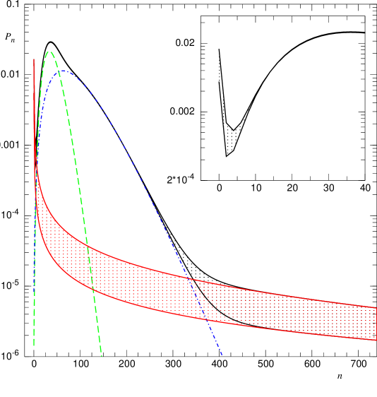
Figure 47: $n$ charged particle multiplicity distribution $P_{n}$ expected at 14 TeV in full phase-space in presence of a third (maybe hard) component with $\bar{N}_{\text{third}}=1$, showing one shoulder structure and one ‘elbow’ structure. The band illustrates the range of values of parameters $\bar{n}_{\text{third}}$, $k_{\text{third}}$ and $\alpha_{\text{third}}$ discussed in the text [108].

Figure 48: Multiplicity distribution in $|\eta|<0.9$ for the scenario described in the text (solid line); the three components are also shown: soft (dashed line), semi-hard (dash-dotted line) and the third (dotted line) [108].

It is assumed therefore that the classes of events contributing to the total sample at 14 TeV are the following:

Class I: soft events (no mini-jets).

$\bar{N}_{\text{soft}}$ is here large and growing with c.m. energy and $\bar{n}_{c,\text{soft}}$ quite small; $P_{n,\text{soft}}$ obeys KNO scaling and $k_{\text{soft}}$ is constant.

Class II: semi-hard events (with mini-jets).

$\bar{N}_{\text{semi-hard}}$ is decreasing with c.m. energy whereas $\bar{n}_{c,\text{semi-hard}}$ is increasing and it larger than $\bar{n}_{c,\text{soft}}$; KNO scaling is violated and $k_{\text{semi-hard}}$ decreases.

Class III: the benchmark of the new class is $k_{\text{third}}<1$.

Being $\bar{N}_{\text{third}}$ (reduced to few units and) approximately equal to 1, quite large forward backward multiplicity correlations are expected and —according to the results of section 4.9 — a leakage parameter from one hemisphere to the opposite one close to its maximum. The fact that hadronic clans are very few with a high particle density per clan should have consequences also at parton level where one should find a huge colour exchange process from a relatively small number of high virtuality ancestors presumably controlled by a mechanism harder than in the components of the other two classes.

Generalising previous results we expect that $P_{n}^{\text{total}}$ be obtained as the weighted superposition of the above mentioned three classes of events each described by a NB (Pascal) MD with characteristic parameters $\bar{n}_{i}$ and $k_{i}$ ($i$ = soft, semi-hard, third) i.e.

$$\begin{split}P_{n}^{\text{total}}&=\alpha_{\text{soft}}P_{n}^{\text{soft}}(\bar{n}_{\text{soft}},k_{\text{soft}})\\ &\quad+\alpha_{\text{semi-hard}}P_{n}^{\text{semi-hard}}(\bar{n}_{\text{semi-hard}},k_{\text{semi-hard}})\\ &\quad+\alpha_{\text{third}}P_{n}^{\text{third}}(\bar{n}_{\text{third}},k_{\text{third}}),\end{split}$$ (184)

with $\alpha_{\text{soft}}+\alpha_{\text{semi-hard}}+\alpha_{\text{third}}=1$ and $\alpha_{\text{soft}}$, $\alpha_{\text{semi-hard}}$ and $\alpha_{\text{third}}$ the weight factors of each class of events with respect to the total sample (see Fig. 47.)

$P_{n}^{\text{total}}$ has a characteristic elbow structure for large $n$ and a narrow peak for $n$ close to zero. Both trends are consequences of the log-convex ($k_{\text{third}}<1$) gamma shape of the $n_{\text{third}}$-charged multiplicity distribution of the new component which shows a high peak at very low multiplicities and a very slow decrease for large ones. The contrast with Pythia Monte Carlo calculations predictions is remarkable as can be seen just by inspection of Figures 45 and 47.

The search on global properties can be extended from full phase-space to rapidity intervals. Since Tevatron data seem to favour, among our scenarios, the one based on strong KNO-scaling violation (i.e., scenario 2 with $k_{\text{total}}^{-1}$ growing linearly in $\ln s$), we decided to discuss in the rapidity interval $|\eta|<0.9$ (which will be available at LHC with Alice detector) this scenario only. The weight factor of each component has been taken to be in the rapidity interval considered the same as in full phase space. Two extreme situations has been allowed for the third component

(i) the third component is distributed uniformly over the whole phase space

(ii) the third component has a very narrow plateau and falls entirely within the interval $|\eta|<0.9$ (see [108] for details.)

Results are shown as a band in Fig. 48. It should be pointed out that the general trend of $P_{n}^{\text{total}}(\eta_{c},\sqrt{s})$ vs. $n$ is quite similar to that already seen in full phase-space. Notice that the narrow peak at very low multiplicity (again due to the third component) is here hidden by the standard peaks of the soft and semi-hard components which are shifted to lower multiplicities than in full phase-space. In order to make the comparison easier, in the following Table are given the parameters for the extrapolated component multiplicity distributions at 14 TeV in full phase-space, assuming that events of the third class comprise 2% of the total:

FPSH	%	$\bar{n}$	$k$	$\bar{N}$	${\bar{n}_{c}}$
soft	41	40	7	13.3	3.0
semi-hard	57	87	3.7	11.8	7.4
third	2	460	0.1212	1	460

and the parameters for the extrapolated component multiplicity distributions at 14 TeV in the pseudo-rapidity interval $|\eta|<0.9$:

$|\eta|<0.9$H	%	$\bar{n}$	$k$	$\bar{N}$	${\bar{n}_{c}}$
soft	41	4.9	3.4	3.0	1.6
semi-hard	57	14	2.0	4.2	3.4
third (i)	2	40	0.056	0.368	109
third (ii)	2	460	0.1212	1	460

(i) events evenly spread over the whole rapidity range

: in this case only 37% of the clan is contained within the pseudo rapidity interval $|\eta|<0.9$, $k_{\text{third}}$ is even much less than 1 and $\bar{n}_{c,\text{third}}\approx 40$.

(ii) event concentrated in $|\eta|<0.9$

: the single clan is fully contained in $|\eta|<0.9$, its parameters are of course the same as those in full phase-space, but particle density in rapidity is much higher than in (i).

The average number of particles per clan both in full phase-space and in the rapidity interval is much larger in the semi-hard than in he soft component (semi-hard clans are larger than soft clans.)

Coming to forward-backward multiplicity correlations, the overall strength for three components is given by

$$b_{\text{FB}}=\frac{\sum_{i=1}^{3}\alpha_{i}\frac{b_{i}D^{2}_{i}}{1+b_{i}}+\frac{1}{2}\sum_{i=1}^{3}\sum_{j>i}^{3}\alpha_{i}\alpha_{j}(\bar{n}_{i}-\bar{n}_{j})^{2}}{\sum_{i=1}^{3}\alpha_{i}\frac{D^{2}_{i}}{1+b_{i}}+\frac{1}{2}\sum_{i=1}^{3}\sum_{j>i}^{3}\alpha_{i}\alpha_{j}(\bar{n}_{i}-\bar{n}_{j})^{2}}.$$ (185)

By taking the quite reasonable assumption that the leakage parameter in $|\eta|<0.9$ is the same as in full phase-space, it has been found:

	FPS	$|\eta|<0.9$
first/soft	0.41	0.25
second/semi-hard	0.51	0.45
third	0.9995	0.997	(i)
		0.9995	(ii)
total (weighted)	0.98	0.92

Notice that $b_{\text{FB,semi-hard}}$ is always larger than $b_{\text{FB,soft}}$. Then $b_{\text{FB,third}}$ tends to saturate in all cases its maximum which is 1.

The total FB multiplicity correlation strength resulting from the weighted superposition of the contributions of all classes of events is larger in FPS than in the rapidity interval but closer to its asymptotic value. As already pointed out, stronger FB correlations at hadron level suggest stronger colour exchange process at parton level and this effect is clearly enhanced in and by the third component.

Clan reduction is an important phenomenon which has already observed in proton-nucleus collisions (see Section 4.3). The attempt is to explore a possible link and to compare predictions in $pp$ collisions with those on nucleus-nucleus collisions in terms of the energy density variable, $\varepsilon$, by using Bjorken formula [109]

$$\varepsilon=\frac{3}{2}\frac{\langle E_{T}\rangle}{V}\left.\frac{dn}{dy}\right|_{y=0},$$ (186)

where $\langle E_{T}\rangle$ is the average transverse energy per particle, $V$ the collision volume and $dn/dy$ the particle density at mid-rapidity. The volume has been estimated with proton radius $\approx 1$ fm and formation time $\tau\approx 1$ fm. Lacking general expectations for $\langle E_{T}\rangle$, for the soft component the value measured at ISR and for the other components the values measured by CDF (which should be intended as a lower bound leading to lower bounds for energy densities as well) has been used. The results are summarised in the following Table:

our scenarios	soft	semi-hard	(i) third (ii)		(i) total (ii)
$dn/dy$	2.5	7	20	230	10.8	19.2
$\langle E_{T}\rangle$ (MeV)	350	500	500	500	500	500
$\varepsilon$ (GeV/fm3)	0.4	1.6	4.7	54	2.5	4.5

The energy density for the semi-hard component in our scenario at 14 TeV is of the same order of magnitude found at AGS at 5.6 GeV in O+Cu collisions ($\varepsilon~{}\approx 1.7$). The energy density for the third component in the spread out scenario is comparable with its value recently measured at RHIC in Au+Au collisions ($\varepsilon~{}\approx 4.6$) The energy density for the third component in the other extreme scenario with high concentration is $\approx 54$, even larger, being $dn/dy$ much larger, than the LHC expectations for Pb+Pb collisions ($\varepsilon~{}\approx 15$)

Of course the above estimate are only indicative, in view of the application of Bjorken formula to $pp$ collisions, as well as for the choice of the values of the parameters. These considerations notwithstanding, it is possible that some characteristic behaviour of observables seen at RHIC in AA collisions could be reproduced at LHC in $pp$ collisions.

5 CONCLUSIONS

Clan concept has been originally introduced in multiparticle phenomenology in order to interpret approximate regularities observed in $n$ charged particle MD’s in all classes of collisions. The occurrence of the same regularity at parton level as a QCD Markov branching process in the solution of KUV differential equations in LLA with a fixed cut-off regularization prescription led to consider partonic clans as independent intermediate gluon sources similar to bremsstrahlung gluon jets.

The sudden violation of the regularity at higher c.m. energies and in larger rapidity intervals in $pp$ collisions and in $e^{+}e^{-}$ annihilation, with the appearance of a shoulder structure in $n$ charged particle MD’s, opened a new horizon in the field and suggested a more accurate search at a deeper level of investigation. The attention on experimental data analysis moved from the full sample of events to the separate samples of events of the single components or substructures of the collisions. It has been an important discovery to find that the same regularity violated in the total sample of events was satisfied in the single components, each described by characteristic and in general different parameters. Their weighted superposition provided a satisfactory understanding of collective variables and correlations behaviours in multiparticle production in the examined classes of collisions where experimental data were available.

Accordingly, clan structure analysis, in view also of its suggestive QCD roots, became an interesting tool in multiparticle dynamics. Furthermore clan existence itself was demanded by a convincing description of forward-backward multiplicity correlations c.m. energy dependence in $pp$ collisions.

The suppression in the same reaction of the average number of clans of the semi-hard component in the TeV energy region in the QCD inspired scenario as well as in the scenario with strong KNO scaling violation (both obtained by extrapolating our knowledge on data in the GeV energy domain), together with the huge increase of the average number of particle per clan, was surprising. It suggested the onset of a new scenario in the TeV energy domain characterised by the appearance of a third class of presumably quite hard events (to be added to the soft and semi-hard ones) with few clans, maybe just one, with the characteristics of high particle density fireballs. The possible anticipation of this new class of events at 14 TeV would be easily experimentally detectable and its finding would shed some light also on the link of $pp$ collisions with heavy ion collisions, where fireballs are expected to be much larger.

Along the years, clans as groups of particles exhausting all correlations inside each clan and generated by independent intermediate particle sources (the clan ancestors) revealed additional properties which helped to make their physical nature more precise, up to the extreme thought that clans might be real physical objects controlling the hadronization process and whose partonic partners might be QCD parton showers originated by intermediate independent gluon sources.

Clan concept turns out to be in this perspective more general than jet concept, in that no kinematical cuts are needed for its definition, and it is also not a purely statistical concept like a standard cluster in cluster expansion in statistical mechanics (as thought at the time of its introduction) in that we learned that a mass can be attributed to clans and that these masses could be quite different in each component and vary from one collision to another one. Assuming that clan existence would be also verified experimentally, a new intriguing question would possibly concern other quantum numbers of these intermediate massive objects occurring in the production process.

In conclusion, it is not clear how far we went in clarifying the enigma of multiparticle dynamics evoked in the introduction to the present paper. This was not indeed our main goal. We wanted to point out how successful and inspiring has been in our search the continuous dialog between theory and experiment and to focus the attention of the reader on the development of a series of experimental facts and theoretical ideas which might, hopefully, transform an enigma in an Arianna thread in the labyrinth of multiparticle dynamics in its awkward journey toward QCD and open new perspectives in $pp$ and heavy ion collisions in the TeV energy domain.

A Physical and mathematical properties of the NB (Pascal) MD

Cornerstone of the present approach to multiparticle dynamics has been the search for regularities of collective variables behaviour in the components or substructures of the various collisions. In view of the relevance in this framework of the NB (Pascal) MD, after some historical notes on its origin and its use, its main mathematical and physical properties, with particular emphasis on clan structure analysis and particle shower development, are summarised for the benefit of the reader. All these properties have been used indeed in the present paper in various occasions and are at the basis of the interpretation of the NB (Pascal) regularity itself.

A.1 Historical notes

A few remarks will help to illustrate the main motivations of the wide use of the negative binomial (Pascal) multiplicity distribution (NB (Pascal) MD) and in more general terms of the class of compound Poisson multiplicity distributions in science.

The NB (Pascal) MD with integer parameter $k$ was known already to Blaise Pascal [110] (that is the reason why it was decided with P. Carruthers [111] few months before his passing, to add the name ‘Pascal’ to the distribution so extensively used in multiparticle dynamics by of all of us.) The distribution appeared fifty years later in the Volume Essay d’analyse sur le jeux de hazard [112]. The front page of the Volume points out that the Volume has been published with the permission of the king Louis XIV and describes the negative binomial as the probability distribution of the number of tosses of a coin necessary to get a fixed number of heads [45]. Gambling was indeed the favourite game of the nobility in that century and the discovery of its statistical rules a real achievement.

The NB (Pascal) MD is used in modern times in many fields (biology, econometrics, medicine…). Its first applications to the spreading of a disease in terms of sickness proneness of various groups of individuals goes back to 1920 and is due to M. Greenwood and G.U. Yule [113].

The distribution appears almost in the same years in quantum statistical mechanics in order to describe $n$ Bose particle multiplicity distribution in $k$ identical systems, each containing on average $\bar{n}/k$ particles [114].

The distribution becomes later of fundamental importance in quantum optics in the study of $n$-photon MD from a partially coherent source [115]; it is remarkable that the photon distribution is Poissonian when the source is coherent ($k=\infty$) and it reduces to a NB (Pascal) MD with $k=1$ (geometric, i.e., Bose-Einstein) when the source is thermal.

After its introduction in high energy collisions in the accelerator region in 1972, the NB (Pascal) MD became quickly —as already pointed out— a stimulating phenomenological tool for describing multiparticle production general trends in all classes of collisions.

Many are the reasons of this success.

Firstly, the NB (Pascal) MD is a compound Poisson distribution and represents one of the the simplest two-parameter MD correcting the independent $n$-particle production process suggested for instance by the multi-peripheral model prediction, i.e., a Poisson multiplicity distribution in the average number of particles $\bar{n}$. The generating function of the NB (Pascal) MD can indeed be written as an exponential of a logarithmic distribution with an intriguing positive numerical factor in front whose interpretation in terms of clan concept is one of the main subject of this review. The reduction of the average population within each clan to one unit, i.e., the equality of the average number of particle of the full distribution with the average number of clans, leads to the Poisson MD of the full $n$-particle distribution. Deviations from unity in the average number of particles per clan represent the correction to the Poissonian behaviour (see Section 2.3.)

Secondly, the NB (Pascal) MD contains a set of multiplicity distributions in correspondence to different limiting values of its standard parameters, as shown in Section A.3, below.

Thirdly, the NB (Pascal) MD is a hierarchical distribution, i.e., all multiplicity correlations can be expressed in terms of second order moments, controlling two-particle correlations (see Section 2.3.)

Fourth, NB (Pascal) MD’s as solutions of the differential QCD evolution equation in LLA can be interpreted as Markov branching processes of two (parton) populations evolving with different strengths (corresponding to the dominant QCD vertices) down to the final (parton) configuration (see Section 3.1.)

A.2 Different parametrisations of the distribution used in multiparticle dynamics

A.2.a

The standard parametrisation of $n$ charged particle multiplicity distribution, $P_{n}$, is usually given in terms of the average charged multiplicity, $\bar{n}$, and the positive parameter $k$, which is linked to the dispersion $D$ of the distribution ($D=\sqrt{\bar{n^{2}}-\bar{n}^{2}}$) by the relation $k=\bar{n}^{2}/(D^{2}-\bar{n})$. $D^{2}$ is therefore larger than $\bar{n}$. Accordingly

$$P_{n}(\bar{n},k)=P_{0}(\bar{n},k)\frac{k(k+1)...(k+n-1)}{n!}\left(\frac{\bar{n}}{\bar{n}+k}\right)^{n},$$ (187)

with

$$P_{0}(\bar{n},k)=\left(\frac{k}{\bar{n}+k}\right)^{k}.$$ (188)

The corresponding generating function is

$$G(\bar{n},k;z)=\sum_{n=0}^{\infty}P_{n}(\bar{n},k)z^{n}=\left[1-\frac{\bar{n}}{k}(z-1)\right]^{-k}$$ (189)

with $G(\bar{n},k;1)=1$ as normalisation condition.

A.2.b

The distribution has been also defined in terms of the coefficients $a$ and $b$ of a linear recurrence relation between $P_{n+1}$ and $P_{n}$ multiplicities, i.e.,

$$(n+1)\frac{P_{n+1}(a,b)}{P_{n}(a,b)}=a+bn,$$ (190)

and $P_{n}(\bar{n},k)$ from above becomes

$$P_{n}(a,b)=P_{0}(a,b)\frac{a(a+b)...(a+b(n-1))}{n!\,b^{n}}$$ (191)

with

$$P_{0}(a,b)=(1-b)^{a/b}.$$ (192)

The corresponding generating function is

$$G(a,b;z)=\sum_{n=0}^{\infty}P_{n}(a,b)z^{n}=\left(\frac{1-b}{1-bz}\right)^{a/b}.$$ (193)

Notice that

$$k=a/b\qquad\text{and}\qquad\bar{n}=a/(1-b).$$ (194)

This definition is particularly suitable in an approach to multiparticle dynamics based on stimulated emission where the parameter $b/a$ corresponds to the fraction of particles already present stimulating the emissions of an additional one [66].

A.2.c

Being the NB (Pascal) MD a compound Poisson distribution, it can be written by using another set of parameters, i.e., the parameters of clan structure analysis $\bar{N}$ (the average number of clans) and $\bar{n}_{c}$ (the average number of particle per clan, $\bar{n}_{c}=\bar{n}/\bar{N}$) and the corresponding generating function turns out to be

$$G(\bar{N},\bar{n}_{c};z)=\exp[\bar{N}(G_{\text{log}}(\bar{n}_{c};z)-1)]$$ (195)

with

$$\bar{N}=k\ln\left(1+\frac{\bar{n}}{k}\right)=-\frac{a}{b}\ln(1-b)$$ (196)

and

$$\bar{n}_{c}=\frac{\bar{n}}{k\ln(1+\bar{n}/k)}=\frac{-b}{(1-b)\ln(1-b)}.$$ (197)

$G_{\text{log}}(\bar{n}_{c};z)$ is the logarithmic multiplicity generating function and is equal to $\ln(1-bz)/\ln(1-b)$. In this framework, $1/k$ is an aggregation parameter, i.e., the ratio between the probability that two particle belong to the same clan to the probability that they belong to different clans [66].

A.2.d

Notice that $G_{\text{log}}(\bar{n}_{c};0)=0$ and that $\exp(-\bar{N})=G(\bar{n},k;0)$. It follows that the zero particle probability is given by

$$\exp(-\bar{N})=P_{0}(\bar{n},k)=\left(\frac{k}{k+\bar{n}}\right)^{k}=(1-b)^{a/b}.$$ (198)

This result can be extended to any interval, $\Delta w$, of a generic variable $w$, (e.g., $w$ could be (pseudo)-rapidity or transverse momentum or coordinate in the real space). In this case the probability to find zero particles in $\Delta w$, $P_{0}(\bar{n}(\Delta w),k(\Delta w))$, is defined and an intriguing connection with clan structure parameters in $\Delta w$ is established, i.e.,

$$\bar{N}(\bar{n}(\Delta w),k(\Delta w))=-\ln P_{0}(\bar{n}(\Delta w),k(\Delta w))$$ (199)

and

$$\bar{n}_{c}(\bar{n}(\Delta w),k(\Delta w))=\frac{1}{V_{0}(\Delta w)},$$ (200)

$V_{0}$ being the void function of Section 2.3.

Of particular interest is indeed the following theorem: factorial cumulant structure is hierarchical, i.e., $n$-order factorial cumulants are controlled by second order factorial cumulants, iff the function $V_{0}(\Delta w)$ scales with energy and $\Delta w$ as a function of $\bar{n}(\Delta w)$ multiplied by the second order factorial cumulant. Being for the NB (Pascal) MD the second order factorial cumulant equal to $1/k(\Delta w)$, it follows that

$$\bar{n}_{c}\left(\frac{\bar{n}(\Delta w)}{k(\Delta w)}\right)=\frac{1}{V_{0}(\Delta w)},$$ (201)

i.e., the distribution is hierarchical, as $K_{n}=f(K_{2})$.

The use of $V_{0}(\Delta w)$ and $P_{0}(\bar{n}(\Delta w),k(\Delta w))$ is of particular interest in the study of rapidity gaps in the various collisions [54].

A.2.e

The NB (Pascal) MD can be obtained also by the weighted superposition of Poissonian MD’s with average multiplicity $\bar{n}_{\lambda}=\lambda\bar{n}$ and gamma weight

$$f(\lambda,k)=\frac{k(\lambda k)^{k-1}}{(k-1)!}\exp(-k\lambda).$$ (202)

It follows

$$\begin{split}P_{n}(\bar{n},k)&=\int_{0}^{\infty}\frac{(\lambda\bar{n})^{n}}{n!}e^{-\bar{n}\lambda}f(k,\lambda)d\lambda\\ &=\left(\frac{k}{\bar{n}+k}\right)^{k}\frac{k(k+1)...(k+n-1)}{n!}\left(\frac{\bar{n}}{\bar{n}+k}\right)^{n}.\end{split}$$ (203)

This representation of the distribution has been used in Section 4.2 in order to describe corrections to the multi-peripheral model predictions. It is known in quantum optics as “Mandel’s equation” [115] and in mathematics as “Poisson transform” with gamma weight [76].

A.2.f

The convolution of two NB (Pascal) MD’s with different parameter $k$ but the same parameter $b$, $P_{n}(k,b)$ and $P_{n^{\prime}}(k^{\prime},b^{\prime})$ is again a NB (Pascal) MD [116]. In fact

$$\begin{split}\sum_{n+n^{\prime}=N}P_{n}(k,b)P_{n^{\prime}}(k^{\prime},b)&=(1-b)^{k+k^{\prime}}b^{N}\frac{(N+k+k^{\prime}-1)!}{N!(k+k^{\prime}-1)!}\\ &=P_{N}(k+k^{\prime},b).\end{split}$$ (204)

A.3 The one-dimensional limits of the parameters of the distribution

A.3.a

The limit $b\to 0$ of $P_{n}(a,b)$ leads to a Poissonian MD:

$$\lim_{b\to 0}P_{n}(a,b)=P_{0}\frac{a^{n}}{n!},$$ (205)

with $P_{0}=e^{-a}$ and in this limit $a=\bar{n}$. i.e.

$$P_{n}(\bar{n})=e^{-\bar{n}}\frac{\bar{n}^{n}}{n!}.$$ (206)

The corresponding generating function (GF) is

$$G(a;z)=\exp[a(z-1)].$$ (207)

Notice that the limit $b\to 0$ corresponds to $a\to\bar{n}$ and $k\to\infty$.

A.3.b

The limit $a\to 0$, with constant $b$, leads to the logarithmic MD:

$$\lim_{a\to 0}P_{n}(a,b)=P_{1}(b)\frac{b^{n-1}}{n},$$ (208)

with $P_{1}(b)=-b/\ln(1-b)$ ($n$ is always $\geq 1$). Therefore

$$P_{n}(b)=-b^{n}/n\ln(1-b).$$ (209)

Notice that this limit corresponds to $k\to 0$, with constant $b$.

A.3.c

The limit $a=b$, i.e., $k=1$, leads to the geometric MD:

$$P_{n}(b,b)=P_{0}(b)b^{n},$$ (210)

with $P_{0}(b)=(1-b)$, and therefore

$$P_{n}(b)=(1-b)b^{n}.$$ (211)

The average multiplicity of the geometric distribution is $b/(1-b)$ and the corresponding GF:

$$G(b;z)=(1-b)/(1-bz).$$ (212)

A.3.d

For $\bar{n}\gg k$ one gets the gamma distribution

$$\lim_{\bar{n}\gg k}P_{n}(\bar{n},k)=\frac{1}{\bar{n}}\frac{k^{k}}{\Gamma(k)}(n/\bar{n})^{k-1}\exp(-kn/\bar{n}).$$ (213)

The distribution is concave for $k>1$ and convex for $k<1$. It becomes an exponential for $k=1$. Notice that $D^{2}/\bar{n}^{2}$ is approximately equal to $1/k$ and that the maximum value of the gamma MD is obtained for $n/\bar{n}=1-1/k$, see [108].

A.3.e

The (positive) binomial limit: For $a>0$ and $b<0$, and $a/b$ an integer number, the negative binomial MD becomes a standard binomial MD and $-k$ (now positive) is the maximum multiplicity. $-1/k$ can be seen as an anti-aggregation parameter, in that particles like to stay far apart from each other.

A.4 Physical informations contained in the differential of the generating function of the multiplicity distribution with respect to its parameters considered as independent variables

Let us consider the differential of the NB (Pascal) MD GF,

$$G(a,b;z)=\left(\frac{1-b}{1-bz}\right)^{a/b},$$ (214)

with respect to its independent variables after the introduction of $\nu=1/(1-b)$ and remembering that $k=a/b$, i.e., the differential of

$$G(a,b;z)=\left(\frac{1}{\nu+z-\nu z}\right)^{k},$$ (215)

with respect to $z$, $\nu$ and $k$ variables, it follows

$$d\ln G(a,b;z)=\frac{a}{1-bz}dz+\ln G(a,b;z)\frac{dk}{k}+k\left[G_{\text{geom}}(\nu;z)-1\right]\frac{d\nu}{\nu-1},$$ (216)

where $G_{\text{geom}}(\nu;z)=(\nu+z-\nu z)^{-1}$ is the GF of the geometric MD.

A.4.a

By taking $k$ and $b$ ($\nu$) constant, the above equation becomes

$$(1-bz)\frac{\partial}{\partial z}G(a,b;z)=aG(a,b;z).$$ (217)

The new equation is the differential form in the generating function language of the linear relation between $n+1$ and $n$ particle MD’s, Eq. (190).

A.4.b

For $z$ and $b$ ($\nu$) constant one obtains that $\ln G(\bar{n},k;z)$ is proportional to $k$:

$$\ln G(\bar{n},k;z)=k\ln G(\bar{n}/k,1;z)$$ (218)

The new equation reminds us in the GF language that the corresponding MD is a CPMD.

A.4.c

By taking $z$ and $k$ constant and integrating the differential between $1$ and $\nu$ one has

$$\ln G(\bar{n},k;z)=k\int_{1}^{\nu}\left[G(\nu^{\prime},z)-1\right]\frac{d\nu^{\prime}}{\nu^{\prime}}.$$ (219)

Notice that for $b=0$ ($\nu=1$) the GF is equal to one. This result is strictly related to the clan structure expressed by the relation

$$G(\bar{n},k;z)=G_{\text{Poisson}}\left(\bar{N};G_{\text{log}}(b;z)\right),$$ (220)

with

$$\bar{N}=k\ln\nu$$ (221)

and

$$G_{\text{log}}(b;z)=\frac{1}{\ln\nu}\int_{1}^{\nu}G_{\text{geom}}(\nu^{\prime};z)d\nu^{\prime}/\nu^{\prime}.$$ (222)

The NB (Pascal) MD is therefore generated by independent emission of geometric clans with mean multiplicity $\nu^{\prime}$ in the interval ($1$, $\nu$) and the average number of geometric clans in ($\nu^{\prime}$ , $\nu^{\prime}+d\nu^{\prime}$) is $kd\nu^{\prime}/\nu^{\prime}$.

It should be pointed out that the GF of the geometric MD, $G_{\text{geom}}(\nu;z)$, obeys the differential equation

$$\nu\frac{\partial}{\partial\nu}G_{\text{geom}}(\nu;z)=G_{\text{geom}}(\nu;z)(G_{\text{geom}}(\nu;z)-1).$$ (223)

In terms of probabilities, it describes a typical self-similar branching process as that found in the Markov process version of the KUV model of gluon shower when the $g\to q\bar{q}$ branching is neglected, as discussed in Section 3.1.

A.5 Informations contained in the differential of the logarithmic MD GF

Let us now consider the GF of the logarithmic MD:

$$G_{\text{log}}(b;z)=\frac{\ln(1-bz)}{\ln(1-b)}.$$ (224)

A simple calculation shows that

$$\begin{split}-(1-b)\ln(1-b)\frac{dG_{\text{log}}(b;z)}{db}&=-G_{\text{log}}(b;z)+\frac{(1-b)z}{1-bz}\\ &=-G_{\text{log}}(b;z)+zG_{\text{geom}}(b;z),\end{split}$$ (225)

or by using the variable $\nu=1/(1-b)$:

$$\ln\nu\frac{dG_{\text{log}}(b;z)}{d\ln\nu}=-G_{\text{log}}(b;z)+zG_{\text{geom}}(b;z).$$ (226)

For an infinitesimal change, the MD of an average clan, which is logarithmic, evolves by addition of a geometric distribution. The first term in the equation is ensuring the normalisation condition $G_{\text{log}}(b;1)=1$. Accordingly, the logarithmic clan can be taken as an average over geometric clans as shown explicitly in Eq. (222).

Contents

1. 1 INTRODUCTION
2. 2 COLLECTIVE VARIABLES AND CLAN STRUCTURE ANALYSIS
   1. 2.1 Observables in multiparticle production. The collective variables.
   2. 2.2 Clan concept and Compound Poisson Multiplicity Distributions.
   3. 2.3 Hierarchical structure of factorial cumulants, rapidity gap events and CPMD’s
   4. 2.4 CPMD’s, truncation and even-odd effects.
3. 3 COLLECTIVE VARIABLES AND QCD PARTON SHOWERS
   1. 3.1 Parton showers in leading log approximation
   2. 3.2 The kinematics problem and possible answers.
      1. 3.2.1 DLA and MLLA and Monte Carlo
      2. 3.2.2 The SPS model
      3. 3.2.3 The GSPS model: generalised clans
   3. 3.3 Hadronization prescriptions
4. 4 COLLECTIVE VARIABLES REGULARITIES IN MULTIPARTICLE PRODUCTION: DATA AND PERSPECTIVES
   1. 4.1 An unsuspected regularity in particle production in cosmic ray physics
   2. 4.2 The occurrence of the NB (Pascal) regularity in full phase-space in the accelerator region and the generalised multiperipheral bootstrap model.
   3. 4.3 The advent of the regularity in different classes of collisions and in rapidity intervals, and its interpretation in terms of clans.
   4. 4.4 The violation of the regularity and its occurrence at a more fundamental level of investigation, i.e., in different classes of events contributing to the total sample in $e^{+}e^{-}$ annihilation and in $pp$ collisions
   5. 4.5 Shoulder effect in $P_{n}$ vs. $n$ at top UA5 energy and in $e^{+}e^{-}$ annihilation and its removal by means of the weighted superposition mechanism of different classes of events
   6. 4.6 $H_{q}$ vs $q$ oscillations and the weighted superposition mechanism
   7. 4.7 Towards the TeV energy domain in $pp$  collisions.
      1. 4.7.1 The average charged multiplicities.
      2. 4.7.2 The $k$ and $k_{i}$ ($i$=soft, semi-hard) parameters.
      3. 4.7.3 Clan structure analysis of $pp$ collisions in the TeV region
      4. 4.7.4 Analysis in pseudo-rapidity intervals
   8. 4.8 Hints from CDF
   9. 4.9 Forward-backward multiplicity correlations. The demand for the existence of clans.
   10. 4.10 Are clans massive objects?
   11. 4.11 The reduction of the average number of clans and signals of new physics in full phase-space and in restricted rapidity intervals
5. 5 CONCLUSIONS
6. A Physical and mathematical properties of the NB (Pascal) MD
   1. A.1 Historical notes
   2. A.2 Different parametrisations of the distribution used in multiparticle dynamics
   3. A.3 The one-dimensional limits of the parameters of the distribution
   4. A.4 Physical informations contained in the differential of the generating function of the multiplicity distribution with respect to its parameters considered as independent variables
   5. A.5 Informations contained in the differential of the logarithmic MD GF
7. ‣ Clan structure analysis and QCD parton showers in multiparticle dynamics. An intriguing dialog between theory and experiment
8. ‣ Clan structure analysis and QCD parton showers in multiparticle dynamics. An intriguing dialog between theory and experiment

References

- [1] E. Fermi, Prog. Theor. Phys. 5, 100 (1950); Phys. Rev. 81, 115 (1951); Phys. Rev. 92, 452 (1953).
- [2] L. Landau, Izv. Akad. Nauk. USSR 17, 51 (1953).
- [3] J.F. Carlson and J.R. Oppenheimer, Phys. Rev. 51, 220 (1937).
- [4] H.J. Bhabha and W. Heitler, Proc. Roy. Soc. 159 A, 432 (1937).
- [5] W.H. Furry, Phys. Rev. 52, 569 (1937).
- [6] J.R. Oppenheimer, H.W. Lewis and S.H. Wouthuysen, Phys. Rev. 73, 127 (1948).
- [7] N. Arley, Proc. Roy. Soc. 168 A, 569 (1937); On the theory of stochastic processes and their application to cosmic rays (John Wiley & Sons, New York, 1931).
- [8] W. Heisenberg, Z. Phys. 113, 61 (1939); W. Heisenberg et al., Vorträge über Kosmische Strahlung (Springer Verlag, Berlin, 1943); W. Heisenberg, Z. Phys. 126, 569 (1949); Z. Phys. 133, 65 (1952).
- [9] S. Fubini, D. Amati and A. Stanghellini, Il Nuovo Cimento 26, 896 (1962).
- [10] G. Wataghin, Anais da Academia Brasileira de Ciências 129 (1942).
- [11] P.K. MacKeown and A.W. Wolfendale, Proc. Phys. Soc. 89, 553 (1966).
- [12] M. Derrick et al., Phys. Rev. Lett. 29, 515 (1972).
- [13] A. Giovannini, Lett. al Nuovo Cimento 6, 514 (1973); Lett. al Nuovo Cimento 7, 35 (1973).
- [14] A. Giovannini et al., Il Nuovo Cimento 24A, 421 (1974); M. Garetto et al., Il Nuovo Cimento 38A, 38 (1977).
- [15] A. Giovannini, Il Nuovo Cimento 10A, 713 (1972); Il Nuovo Cimento 15A, 543 (1973).
- [16] G.J. Alner et al. (UA5 Collaboration), Phys. Lett. B160, 193 (1985).
- [17] M. Adamus et al., NA22 Collaboration, Phys. Lett. B177, 239 (1986).
- [18] M. Derrick et al., HRS Collaboration, Phys. Lett. B168, 299 (1986).
- [19] A. Breakstone et al., Il Nuovo Cimento 102A, 1199 (1989).
- [20] W. Braunschweig et al., TASSO Collaboration, Z. Phys. C45, 193 (1989).
- [21] M. Arneodo et al., EMC Collaboration, Z. Phys. C35, 335 (1987).
- [22] L. Van Hove and A. Giovannini, in XVII International Symposium on Multiparticle Dynamics, edited by M. Markitan et al (World Scientific, Singapore, 1987), p. 561.
- [23] A. Giovannini, Nucl. Phys. B161, 429 (1979).
- [24] K. Konishi, A. Ukawa and G. Veneziano, Nucl. Phys. B157, 45 (1979).
- [25] W. Kittel, in Workshop on Physics with Future Accelerators, edited by J. Mulvay (CERN, Yellow Rep. 87-7, 1987), Vol. II, p. 424.
- [26] L. Van Hove and A. Giovannini, Acta Phys. Pol. B 19, 917 (1988).
- [27] R.E. Ansorge et al. (UA5 Collaboration), Z. Phys. C 43, 357 (1989).
- [28] P. Abreu et al. (DELPHI Collaboration), Z. Phys. C 50, 185 (1991).
- [29] P. Abreu et al. (DELPHI Collaboration), Z. Phys. C 52, 271 (1991).
- [30] P. Abreu et al. (DELPHI Collaboration), Z. Phys. C56, 63 (1992).
- [31] A. Giovannini, S. Lupia and R. Ugoccioni, Nucl. Phys. (Proc. Suppl.) B25, 115 (1992).
- [32] A. Giovannini, S. Lupia and R. Ugoccioni, Phys. Lett. B 374, 231 (1996).
- [33] A. Giovannini and R. Ugoccioni, Phys. Rev. D 66, 034001 (2002).
- [34] S. J. Lee and A. Z. Mekjian, Nucl. Phys. A 730, 514 (2004); H. Nakamura and R. Seki, Phys. Rev. C 66, 024902 (2002); C. E. Aguiar and T. Kodama, Physica A 320, 371 (2003); A. Z. Mekjian, Phys. Rev. C 65, 014907 (2002); M. Martinis and V. Mikuta-Martinis, Fizika B 5, 269 (1996); G. Calucci and D. Treleani, Phys. Rev. D 57, 602 (1998).
- [35] D. Ghosh, A. Deb, S. Bhattacharyya, and J. Ghosh, Phys. Rev. C 69, 027901 (2004); M.M. Aggarwal et al. (WA98 Collaboration), Phys. Rev. C 65, 054912 (2002); T. Abbott et al., Phys. Rev. C 63, 064602 (2001); A. Z. Mekjian, B. R. Schlei, and D. Strottman, Phys. Rev. C 58, 3627 (1998).
- [36] T. Osada, M. Maruyama, and F. Takagi, Phys. Rev. D 59, 014024 (1999); D.-w. Huang, Phys. Rev. D 55, 5845 (1997); P. Achard et al., Phys. Lett. B 577, 109 (2003); P. Abreu et al., Phys. Lett. B 457, 368 (1999).
- [37] K. Boruah, Phys. Rev. D 56, 7376 (1997); S. V. Chekanov, Eur. Phys. J. C 6, 331 (1999); S. Aid et al., Z. Phys. C 72, 573 (1996); E. Kokoulina, Acta Phys. Pol. B 35, 295 (2004).
- [38] Z. Koba, in 1973 CERN - JINR School of Physics (CERN, Yellow Rep. 73-12, 1973), p. 171.
- [39] S. Lupia, Ph.D. thesis, University of Torino, 1995.
- [40] E.A. De Wolf, I.M. Dremin and W. Kittel, Physics Reports 270, 1 (1996).
- [41] P. Carruthers, Phys. Rev. A43, 2632 (1991).
- [42] C. Fuglesang, in Multiparticle Dynamics: Festschrift for Léon Van Hove, edited by A. Giovannini and W. Kittel (World Scientific, Singapore, 1990), p. 193.
- [43] I.M. Dremin, Phys. Lett. B 313, 209 (1993).
- [44] M. Kendall and A. Stuart, The advanced theory of statistics (4th edition, Griffin & Co. Lim., London).
- [45] N.L. Johnson, S. Kotz and A.W. Kemp, Univariate discrete distributions (2nd edition, J. Wiley & Sons, New York).
- [46] W. Feller, An introduction on probability theory and its applications (Vol. I, 3rd ed., J. Wiley & Sons).
- [47] S. Hegyi, Phys. Lett. B271, 214 (1992); Phys. Lett. B318, 642 (1993).
- [48] I.M. Dremin and R.C. Hwa, Phys. Rev. D49, 5805 (1994).
- [49] P.J.E. Peebles, The large scale structure of the universe (Princeton University Press, New York, 1980).
- [50] S. Lupia, A. Giovannini and R. Ugoccioni, Z. Phys. C59, 427 (1993).
- [51] P. Carruthers and I. Sarcevic, Phys. Rev. Lett. 63, 1562 (1989).
- [52] L. Van Hove, Phys. Lett. B 242, 485 (1990).
- [53] J.D. Bjorken, Phys. Rev. D47, 101 (1993).
- [54] S. Lupia, A. Giovannini and R. Ugoccioni, Z. Phys. C66, 195 (1995).
- [55] D.-w. Huang, Phys. Rev. D 58, 017501 (1998).
- [56] Yu.L. Dokshitzer, V.A. Khoze, A.H. Mueller and S.I. Troyan, Basics of perturbative QCD (Editions Frontières, Gif-sur-Yvette, 1991).
- [57] I. M. Dremin and J. W. Gary, Physics Reports 349, 301 (2001).
- [58] V. A. Khoze and W. Ochs, Int. J. Mod. Phys. A12, 2949 (1997).
- [59] Z. Koba, H.B. Nielsen and P. Olesen, Nucl. Phys. B40, 317 (1972).
- [60] Yu.L. Dokshitzer, Phys. Lett. B305, 295 (1993).
- [61] R. Ugoccioni, A. Giovannini and S. Lupia, Phys. Lett. B 342, 387 (1995).
- [62] K. Abe et al., SLD Collaboration, Phys. Lett. B371, 149 (1996).
- [63] R. Ugoccioni and A. Giovannini, Z. Phys. C53, 239 (1992).
- [64] R. Ugoccioni, A. Giovannini and S. Lupia, Z. Phys. C64, 453 (1994).
- [65] A. Giovannini, S. Lupia and R. Ugoccioni, Z. Phys. C70, 291 (1996).
- [66] A. Giovannini and L. Van Hove, Z. Phys. C 30, 391 (1986).
- [67] F. Bianchi, A. Giovannini, S. Lupia and R. Ugoccioni, Z. Phys. C 58, 71 (1993).
- [68] A. Giovannini and L. Van Hove, Acta Phys. Pol. B 19, 931 (1988).
- [69] B. Andersson, The Lund Model (Cambridge University Press, Cambridge, U.K., 1996).
- [70] G. Marchesini and B.R. Webber, Nucl. Phys. B 310, 461 (1988).
- [71] F. Becattini, Z. Phys. C 69, 485 (1996); F. Becattini and U.W. Heinz, Z. Phys. C 76, 269 (1997).
- [72] L. Van Hove, Physica 147A, 19 (1987).
- [73] J. Finkelstein, Phys. Rev. D37, 2446 (1989).
- [74] F. Becattini, A. Giovannini and S. Lupia, Z. Phys. C 72, 491 (1996).
- [75] W. Kittel, in Multiparticle Dynamics: Festschrift for Léon Van Hove, edited by A. Giovannini and W. Kittel (World Scientific, Singapore, 1990), p. 323.
- [76] P. Carruthers and C.C. Shih, Int. J. Mod. Phys. A2, 1447 (1987).
- [77] G.J. Alner et al. (UA5 Collaboration), Phys. Lett. B160, 199 (1985).
- [78] G.J. Alner et al. (UA5 Collaboration), Physics Reports 154, 247 (1987).
- [79] L. Van Hove and A. Giovannini, invited talk, in 25th International Conference on High Energy Physics, edited by K.K. Phua and Y. Yamaguchi (World Scientific, Singapore, 1991), p. 998.
- [80] G. Giacomelli and M. Jacob, Physics Reports 55, 1 (1979).
- [81] N. Schmitz, in Multiparticle Dynamics: Festschrift for Léon Van Hove, edited by A. Giovannini and W. Kittel (World Scientific, Singapore, 1990), p. 25.
- [82] M. Adamus et al., NA22 Collaboration, Phys. Lett. B B177, 239 (1986); Phys. Lett. B205, 401 (1988); Z. Phys. C32, 475 (1986); Z. Phys. C37, 215 (1988).
- [83] T. Sjöstrand and M. Bengstsson, Computer Physics Commun. 82, 74 (1994).
- [84] F. Dengler et al., Z. Phys. C 33, 187 (1986); J.L. Bailly et al. (EHS-RCBC Collaboration), Z. Phys. C C40, 215 (1988).
- [85] J. Bächler at el., NA35 Collaboration, Z. Phys. C57, 541 (1993).
- [86] M. Tannenbaum, in XXIII International Symposium on Multiparticle Dynamics, edited by M. Block and A. White (World Scientific, Singapore, 1994), p. 261; M. Tannenbaum, Mod. Phys. Lett. A9, 89 (1994).
- [87] I.M. Dremin et al., Phys. Lett. B336, 119 (1994).
- [88] P. Abreu et al., DELPHI Collaboration, Z. Phys. C 70, 179 (1996).
- [89] R. Akers et al. (OPAL Collaboration), Phys. Lett. B320, 417 (1994).
- [90] G. Ciapetti (UA1 Collaboration), in 5th Topical Workshop on Proton-Antiproton Collider Physics, edited by M. Greco (World Scientific, Singapore, 1986), p. 488.
- [91] C. Albajar et al., UA1 Collaboration, Nucl. Phys. B309, 405 (1988).
- [92] A. Giovannini, S. Lupia e R. Ugoccioni, in 7th International Workshop “Correlations and Fluctuations”, edited by R.C. Hwa, W. Kittel, W.J. Metzger and D.J. Schotanus (World Scientific, Singapore, 1997), p. 328.
- [93] A. Giovannini and R. Ugoccioni, Phys. Rev. D 59, 094020 (1999).
- [94] A. Giovannini and R. Ugoccioni, Phys. Rev. D 60, 074027 (1999).
- [95] T. Alexopoulos et al. (E735 Coll.), Phys. Lett. B435, 453 (1998).
- [96] J. Dias de Deus and R. Ugoccioni, Phys. Lett. B469, 243 (1999).
- [97] S.G. Matinyan and W.D. Walker, Phys. Rev. D59, 034022 (1998).
- [98] A. Del Fabbro and D. Treleani, Nucl. Phys. Proc. Suppl. 92, 130 (2001).
- [99] D. Acosta et al. (CDF Collaboration), Phys. Rev. D 65, 072005 (2002).
- [100] A. Giovannini and R. Ugoccioni, J. Phys. G 28, 2811 (2002).
- [101] J. Dias de Deus, J. Kwiecinski and M. Pimenta, Phys. Lett. B202, 397 (1988).
- [102] P. Carruthers and C.C. Shih, Phys. Lett. B165, 209 (1985).
- [103] A. Giovannini and R. Ugoccioni, Phys. Lett. B 558, 59 (2003).
- [104] T.T. Chou and C.N. Yang, Phys. Lett. B135, 175 (1984); Phys. Rev. D 32, 1692 (1985).
- [105] T. Alexopoulos et al., Phys. Lett. B 528, 43 (2002).
- [106] A. Białas and A. Szczerba, Acta Phys. Pol. B 17, 1085 (1986).
- [107] A. Giovannini and R. Ugoccioni, J. Phys. G 29, 777 (2003).
- [108] A. Giovannini and R. Ugoccioni, Phys. Rev. D 68, 034009 (2003).
- [109] J.D. Bjorken, Phys. Rev. D27, 140 (1983).
- [110] B. Pascal, Varia Opera Mathmatica D. Petri de Fermat (Tolossae, 1679).
- [111] P. Carruthers, University of Arizona preprint No. AZPH-TH-94-10.
- [112] P.R. Montmort, Essay d’analyse sur le jeux de hazard (Quillou, Paris, 1713).
- [113] M. Greenwood and G.U. Yule, J. Royal Statistical Society A 83, 255 (1920).
- [114] M. Planck, Sitzungber. Deutsch. Akad. Wiss. Berlin 33, 355 (1923).
- [115] L. Mandel, Proc. Phys. Soc. London 233 (1959).
- [116] L.-N. Chang and N.-P. Chang, Phys. Rev. D 9, 660 (1974).