Vector Meson Contributions in $\epsilon^{\prime}/\epsilon$

Abstract

The CP violating parameter $\varepsilon^{\prime}/\varepsilon$ is computed using the low-energy dynamics of the chiral theory supplemented by vector resonances. The divergent contributions coming from strong $\pi$-$\pi$ scattering are tamed by vector-meson exchange terms. This amounts to softening the fast growing high-energy behaviour of $\pi$-$\pi$ scattering. The final result for $\epsilon^{\prime}/\epsilon$ shows a smooth dependence on the cut-off where low energy dynamics is matched with that of QCD.

1. Introduction. The decays $K\to\pi\pi$ are best described by a low energy effective Hamiltonian

$$H=\frac{G_{F}}{\sqrt{2}}\xi_{u}\left\{\sum_{i=1}^{8}(z_{i}(q^{2},\mu^{2})+\tau y_{i}(q^{2},\mu^{2}))Q_{i}\right\}$$ (1)

with $z_{i}(q^{2},\mu^{2})$ and $y_{i}(q^{2},\mu^{2})$ being the Wilson coefficients and $\xi_{q}=V^{*}_{qs}V_{qd}$, $\tau=\xi_{t}/\xi_{u}$ . $Q_{i}$’s are 4-quark operators. For the definition of the operators and other notations, see ref. Hambye:PRD which we closely follow. Matrix elements for two of these operators, $Q_{6}$ and $Q_{8}$, are most important for the evaluation of $\varepsilon^{\prime}/\varepsilon$:

$$Q_{6} = -2\sum_{q=u,d,s}\bar{s}(1+\gamma_{5})q\bar{q}(1-\gamma_{5})d,$$

$$Q_{8} = -3\sum_{q=u,d,s}e_{q}\bar{s}(1+\gamma_{5})q\bar{q}(1-\gamma_{5})d,$$ (2)

where $e_{q}=(2/3,-1/3,-1/3)$. The QCD corrections included in the Wilson coefficients represent the short distance terms computed in perturbative QCD. They depend on $[\ln(Q^{2}/\mu^{2})]^{\gamma/\beta}$ and to next-to-leading order (NLO) corrections in a more complicated way. The numerical values have been tabulated by various groups ref1 ; ref2 . Comparisons of the results show that the various groups agree with each other but values for the coefficients depend on the renormalization scheme. The $\mu$-dependence in the coefficients is expected to be cancelled by the scale dependence of the matrix elements of the operators introduced through the upper cut-off in the integrals, and the running strange quark mass.

The matrix elements of the form $\langle\pi\pi|Q_{6}|K\rangle$ and $\langle\pi\pi|Q_{8}|K\rangle$ include tree level contributions and loop corrections. These are low energy processes which must be dealt with by methods other than QCD. Our method is to use the low energy chiral theory for calculating tree and loop diagrams and then match the results with the short distance contribution, i.e. the QCD scale $\mu$ is matched with the upper cut-off $\Lambda_{c}$ appearing in the chiral loops. An important criterion for the success of the calculation is smooth (and weak) dependence of the results on $\mu=\Lambda_{c}$.

In the large $N_{c}$ approach factorizable and non-factorizable amplitudes are treated separately BBG with the factorizable amplitudes defining the renormalized coupling constants. In a Dortmund-Fermilab collaboration Hambye:PRD , it was shown that to $\mathcal{O}(p^{0}/N_{c})$ the divergences in the matrix elements of the $Q_{6}$ and $Q_{8}$ operators are logarithmic and occur in nonfactorizable diagrams.

The numerical results of this approach at $\mathcal{O}(p^{0}/N_{c})$ were presented in table I of ref.Hambye:PRD , which we also adopt in the present article. The results of the diagrammatic method were reproduced in the background-field method Hambye:NPB . Let us denote the nonet of pseudoscalar meson by the matrix $\Pi=P_{a}\lambda^{a}$, where $\lambda_{a}$’s are the usual Gell-Mann matrices; then it was shown that to $O(p^{0}/N_{c})$

$${\pi_{0}\over f}={\pi_{r}\over F_{\pi}}\ \ {\rm and}\ \ {K_{0}\over f}={K_{r}\over F_{K}}$$ (3)

where $(\pi_{0},K_{0})$ and $f$ are the bare pion and kaon fields and decay constants, while $(\pi_{r},K_{r})$ and $F_{\pi},F_{K}$ are renormalized fields and decay constants, respectively.

A large correction in the earlier calculation Hambye:NPB originates from rescattering of the pions, i.e., $K\to\pi\pi\to\pi\pi$

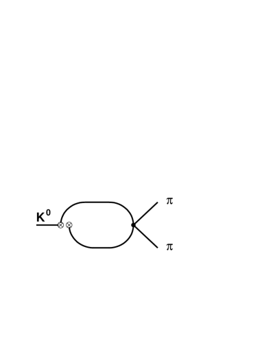
Figure 1: Feynman diagram for $K\to\pi\pi$ with strong final state interactions.

where the first step involves the weak operators $Q_{6}$ or $Q_{8}$ to $\mathcal{O}(p^{2}/N_{c})$ and the second process is the strong pion-pion scattering as shown in Fig. 1. The large dependence of the cut-off resides on the contact $\pi-\pi$ scattering which is known to have a bad high-energy behaviour violating unitarity and needs to be moderated by some other amplitudes which restore unitarity.

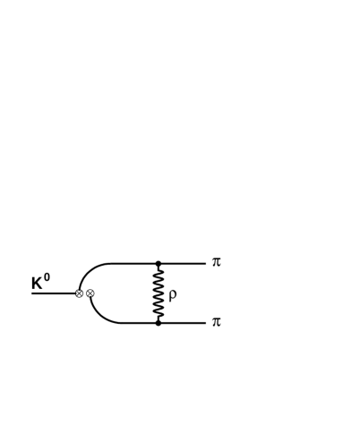
Figure 2: Feynman diagram for $K\to\pi\pi$ with a vector-meson exchange.

A standard prescription to restore unitarity is to introduce vector-meson exchange diagrams. For the $\pi\pi\to\pi\pi$ scattering we shall use the contact and the $\rho$ exchange diagrams. We accomplish this by using a chiral Lagrangian for pseudo scalars and enlarged by the introduction of vector mesons Bando ; ref5 ; ref5b . We extend the calculation of the one-loop diagrams with a strong vertex with the addition of a $\rho$-exchange diagram. The $\rho$ is included to represent the effects of even heavier vector mesons (like $K^{*}$). In addition the pions are in $I=0$ or $I=2$ states and the exchange of $\rho$-mesons appears only in the $t$-channel, see Fig.2.

In order to restore unitarity we shall demand that quadratic divergences cancel between the contact and the $\rho$-exchange diagrams. It is indeed heartening to note that they come with opposite signs, and cancel exactly if the following relation is satisfied

$$\frac{h^{2}}{m^{2}_{\rho}}=\frac{1}{3f^{2}}\,.$$ (4)

Here $h$ is the $\rho\pi\pi$ coupling strength and $f$ is the pion decay constant ($\approx 92MeV$). The logarithmic divergences still remain and should be matched to the QCD logarithms. This is our proposal for moderating the high energy growth of $\pi-\pi$ scattering.

Thus, we calculate the one-loop $K\to\pi\pi$ amplitudes with both contact and $\rho$-exchange diagrams, demanding that the quadratic divergences cancel betwen these two sets. The value of $h\simeq 4.8$ obtained from Eq.(4) is slightly smaller than the one obtained from the $\rho$ decay width, but remember that $\rho$ is only a symbolic representation of all possible vector resonances. Since only logarithmic divergences will be present in the final result, the variation of $\varepsilon^{\prime}/\varepsilon$ with the cut-off $\Lambda$ is expected to be weak. As the weak vertex (with $Q_{6}$ or $Q_{8}$) is common to both the contact and the $\rho$-exchange diagrams, the cancellation of quadratic divergences is respected by both operators.

2. Framework. The effective Lagrangian for pseudoscalar mesons relevant for $K\to\pi\pi$ decay up to ${\cal O}(p^{4})$ is given by gasser-leutwyler :

$${\cal L}_{eff} = {f^{2}\over 4}\left(\langle\partial_{\mu}U^{\dagger}\partial^{\mu}U\rangle+{\alpha\over 4N_{c}}\langle\ln U^{\dagger}-\ln U\rangle^{2}+r\langle{\cal M}U^{\dagger}+UM\rangle\right)+r^{2}H_{2}\langle M^{2}\rangle$$ (5)

$$+rL_{5}\langle\partial_{\mu}U^{\dagger}\partial^{\mu}U\left(MU+U^{\dagger}M\right)\rangle+r^{2}L_{8}\langle MUMU+MU^{\dagger}MU^{\dagger}\rangle,$$

with $\langle A\rangle$ denoting the trace of $A$ and $M={\rm diag}(m_{u},m_{d},m_{s})$, $f$ and $r$ are free parameters related to the pion decay constant $F_{\pi}$ and to the quark condensate respectively, with $r=-2\langle\bar{q}q\rangle/f^{2}$.

The matrix $U$ is given by

$$U=\exp(i\Pi/f),$$ (6)

where the pseudoscalar meson nonet $\Pi$ is given by

$$\Pi=\lambda^{a}P_{a}=\begin{pmatrix}\pi^{0}+{1\over\sqrt{3}}a\eta+{\sqrt{2}\over\sqrt{3}}b\eta^{\prime}&\sqrt{2}\pi^{+}&\sqrt{2}K^{+}\cr\sqrt{2}\pi^{-}&-\pi^{0}+{1\over\sqrt{3}}a\eta+{\sqrt{2}\over\sqrt{3}}b\eta^{\prime}&\sqrt{2}K^{0}\cr\sqrt{2}K^{-}&\sqrt{2}\bar{K^{0}}&-{2\over 3}b\eta+{\sqrt{2}\over\sqrt{3}}a\eta^{\prime}\end{pmatrix}$$ (7)

where $\lambda$’s are the usual Gell-Mann matrices, $P_{a}$ are the pseudoscalar fields, and

$$a=\cos\theta-\sqrt{2}\sin\theta,\ \ b={1\over\sqrt{2}}\sin\theta+\cos\theta,$$ (8)

$\theta$ being the $\eta-\eta^{\prime}$ mixing angle. We include $\eta$ and $\eta^{\prime}$ contributions in our calculation. It is easy to see that though the operator $Q_{6}$ vanishes at tree-level due to the unitarity of $U$, it still has nonzero contributions at the $\mathcal{O}(p^{0}/N_{C})$ level. The loop expansion of the matrix elements is a series in $1/f^{2}\sim 1/N_{c}$, which follows from the short-distance expansion in terms of $\alpha_{s}/\pi\sim 1/N_{c}$.

There have been numerous calculations of $\varepsilon^{\prime}/\varepsilon$ which try to improve various steps epsilonP . The expression of $\epsilon^{\prime}/\epsilon$ can be written in a compact notation as

$${\varepsilon^{\prime}\over\varepsilon}={G_{F}\over 2}{\omega\over|\varepsilon|{\rm Re}A_{0}}{\rm Im}\xi_{t}\left[\Pi_{0}-{1\over\omega}\Pi_{2}\right],\qquad(\omega=1/22)$$ (9)

with

$$\Pi_{0} = |\sum_{i}y_{i}(\mu)\langle Q_{i}\rangle_{0}|\left(1-\Omega_{\eta+\eta^{\prime}}\right),$$

$$\Pi_{2} = |\sum_{i}y_{i}(\mu)\langle Q_{i}\rangle_{2}|.$$ (10)

The isospin breaking effect ($m_{u}\not=m_{d}$) is taken into account by $\Omega_{\eta+\eta^{\prime}}$.

Our aim is to introduce vector mesons in terms of a Lagrangian which satisfies the low energy current algebra. One consistent method is in terms of a non-linear chiral Lagrangian with a hidden local symmetry Bando . In this theory the vector mesons emerge as dynamical vector mesons. The three point vector-pseudo scalar interaction is given by

$$\frac{ih}{4}\langle V_{\mu}(P\partial^{\mu}P-\partial^{\mu}PP)\rangle,$$ (11)

where $h$ stands for the vector-pseudoscalar coupling. Some typical vertices of $\rho$’s to pseudoscalar mesons are

$$\pi^{+}(p_{1})\pi^{-}(p_{2})\rho^{0} :h(p_{1}-p_{2})_{\mu}\epsilon^{\mu}$$

$$\pi^{+}(p_{1})\pi^{0}(p_{2})\rho^{-} :h(p_{1}-p_{2})_{\mu}\epsilon^{\mu}$$

$$K^{+}(p_{1})\bar{K}^{0}(p_{2})\rho^{-} :\frac{h}{\sqrt{2}}(p_{1}-p_{2})_{\mu}\epsilon^{\mu},\quad etc,$$ (12)

which is directly related to the $\rho$ decay width: $\Gamma(\rho)=h^{2}(|\mathbf{p}_{\pi}|)^{3}/(6\pi m_{\rho}^{2})$, where $\mathbf{p}_{\pi}$ is the momentum of final state pions in the $\rho$ rest frame. With $\Gamma(\rho)=149.2$ MeV, we find $h=5.95$. We note in passing that the Kawarabayashi-Suzuki-Riazuddin-Fayyazuddin relation gives the value $h=m_{\rho}/(\sqrt{2}f_{\pi})$KSRF . Thus the value of $h$ in Eq.(4) and the two values in this paragraph differ by small amounts $(\sim 19\%)$. The strong four-point vertices involving pions are obtained from the first two terms of Eq. (5). The weak vertices are obtained from the definitions of $Q_{6}$ and $Q_{8}$. In the numerical work we shall use the value of $h$ from Eq.(4) and also $h=5.95$ obtained from the decay width.

We repeated the renormalization procedure and found the following results. For the self energies of the pseudoscalars, momentum independent terms combine with the bare masses to define the physical masses. A momentum dependent term is included in the wave function renormalization and is the same for $\pi$ and $K$. The renormalization of $F_{\pi}$ and $F_{K}$ is the same as in ref.Hambye:PRD , i.e. there is no $h^{2}$ contribution, which leads to the same value for $L_{5}$, similarly the value for $L_{5}-2L_{8}$ is again very small. The quadratic divergences of the factorizable diagrams for $\langle Q_{6}\rangle_{0}$, $\langle Q_{6}\rangle_{2}$ and $\langle\pi^{0}\pi^{0}|Q_{8}|K\rangle$ cancel out, what remains of them are small corrections because to $\mathcal{O}(p^{0})$ these matrix elements vanish. The quadratic divergence from the factorizable diagrams of $\langle\pi^{+}\pi^{-}|Q_{8}|K\rangle$ cancel against the corresponding diagrams with vector meson exchanges when we invoke the condition in Eq.(4). The surviving term is small in comparison with the $\mathcal{O}(p^{0})$ contribution of $\langle\pi^{+}\pi^{-}|Q_{8}|K\rangle$.

We use the following numerical inputs:

$$m_{\pi} =0.137\mbox{GeV}, m_{K} =0.495\mbox{GeV}, m_{\rho} =0.771\mbox{GeV},$$

$$f \equiv F_{\pi}=0.0924, m_{s}(m_{c}) =0.115\mbox{GeV}, \alpha_{S}(m_{Z}) =0.117.$$ (13)

The strange quark mass has an error of 0.020 GeV Buras:03 . The average quark mass $\hat{m}$ is given by $\hat{m}=m_{s}/24.4$. We also use $\hat{L_{5}}=2.07\times 10^{-3}$, $\hat{L_{8}}=1.09\times 10^{-3}$, $Im(\xi_{t})=(1.31\pm 0.10)\times 10^{-4}$Hambye:PRD and the isospin breaking factor of $\Omega_{\eta+\eta^{\prime}}=0.15$ isospinBRK .

One can extract $\Lambda^{(4)}_{QCD}$ from $\alpha_{S}(m_{Z})$ at either the continuum upper limit PDG ($\bar{m_{b}}(\bar{m_{b}})=4.5$ GeV, $\bar{m_{c}}(\bar{m_{c}})=1.4$ GeV) or the continuum lower limit ($\bar{m_{b}}(\bar{m_{b}})=4.0$ GeV, $\bar{m_{c}}(\bar{m_{c}})=1.0$ GeV):

$$\Lambda^{(4)}_{QCD}=0.279\pm 0.029({\rm upper~{}limit}),\ \ \Lambda^{(4)}_{QCD}=0.275\pm 0.029({\rm lower~{}limit}).$$ (14)

We take, as a conservative estimate, $\Lambda^{(4)}_{QCD}=0.277\pm 0.031$ GeV (i.e., between 0.246 and 0.308 GeV).

The Wilson coefficients were tabulated Hambye:NPB for various renormalization schemes and the values of $\Lambda^{(4)}_{QCD}$ as functions of the renormalization scale $\mu$. The values show a convergence among the schemes as $\mu$ increases and approaches the value of $\mu=1$ GeV. This is as expected since QCD is valid at higher momenta.

A second issue is the matching of the coefficients in the various schemes to the cut-off scale of chiral theory. A method for relating the two scales was suggested in Bardeen:2001kd . The method introduces

$$1=\frac{q^{2}}{q^{2}-m^{2}}-\frac{m^{2}}{q^{2}-m^{2}}$$ (15)

and uses the first term as the infrared regulator of QCD and the second term as the cut-off for the chiral theory. This approach provides a matching of the two scales $\Lambda_{c}$ and $\mu$. Recalculation of the evolution of the coefficients Bardeen:2001kd brings the values of the HV scheme closer to NDR, which are anyway close to the leading order results. All this motivates us to use the values of the NDR scheme. We shall use values for $\Lambda^{(4)}_{QCD}=0.245$ GeV, however, we check that interpolation to $\Lambda^{(4)}_{QCD}=0.277\pm 0.031$ GeV changes the values of $\epsilon^{\prime}/\epsilon$ at most $8\%$. Althernative ways for matching the two theories have also been introduced in other articles Wu-match .

3. Results. As mentioned already, a previous work demonstrated that renormalization of physical quantities (wave functions, masses and decay constants) render the factorizable contribution to $\langle Q_{6}\rangle_{0,2}$ and $\langle Q_{8}\rangle_{0,2}$ to ${\cal O}(p^{0}/N_{C})$ finite. There are loop corrections introduced by the non-factorizable diagrams which to order $p^{0}/N_{C}$ were found to be logarithmic. Going one step further corrections of order $p^{2}/N_{C}$ were studied Hambye:NPB , arising from the contact terms which have a quadratic dependence on the cut-off scale $\Lambda^{2}_{c}$. We combine the contact terms with the vector meson exchange diagrams and cancel the quadratic divergence.

We present in this section the results for the contact terms and vector meson exchange diagrams to order $p^{2}/N_{C}$ in terms of integrals which are summarized in Appendix A. In order to make the reading easier we give in the text explicit formulas for the decay $K^{0}\rightarrow\pi^{0}\pi^{0}$ where the results are shorter. For the decay of $K^{0}\rightarrow\pi^{+}\pi^{-}$ we collected the results in Appendix B. In both reactions we included the $\pi^{+}\pi^{-}$ and $\pi^{0}\pi^{0}$ intermediate states.

The contact terms for $K^{0}(p_{K})\rightarrow\pi^{+}\pi^{-}\rightarrow\pi^{0}\pi^{0}$ give

$$i{\mathcal{M}}^{00}_{\operatorname{con1}} = i\frac{2r^{2}}{3\sqrt{2}f^{3}}[AI_{9}(m_{\pi},m_{\pi},p_{K},p_{K})+BI_{11}(m_{\pi},m_{\pi},p_{K},p_{K},p_{K})$$ (16)

$$-AI_{10}(m_{\pi},m_{\pi},p_{K})-BI_{12}(m_{\pi},m_{\pi},p_{K},p_{K})$$

$$+ACI_{8}(m_{\pi},m_{\pi},p_{K})+BCI_{9}(m_{\pi},m_{\pi},p_{K},p_{K})]$$

with $A=-8L_{5}m_{K}^{2},B=8L_{5},C=(\chi_{1}+\chi_{2})/4+m_{K}^{2}-m_{\pi}^{2}$ and $\chi_{i}=rm_{i}$.

The contact term for $K^{0}(p_{K})\rightarrow\pi^{0}\pi^{0}\rightarrow\pi^{0}\pi^{0}$ is

$$i{\mathcal{M}}^{00}_{\operatorname{con2}} = i\frac{r^{2}}{4\sqrt{2}f^{3}}C^{\prime}[AI_{8}(m_{\pi},m_{\pi},p_{K})+BI_{9}(m_{\pi},m_{\pi},p_{K},p_{K})]$$ (17)

with $C^{\prime}=(\chi_{1}+\chi_{2})$ . The functions $I_{i}(m_{j},m_{k},p,\dots)$ etc represent four dimensional integrals which we define in the Appendix A. The notation with the numbers as subscripts follow the convention introduced in two Ph.D. theses at Dortmund UniversityKohler+Soldan , where explicit formulas for the functional forms after integration are included.

The $\rho-$exchange diagram for $K^{0}(p_{K})\rightarrow\pi^{+}\pi^{-}\rightarrow\pi^{0}\pi^{0}$ is

$$i{\mathcal{M}}^{00}_{\operatorname{exch}1} = (-i)\frac{2h^{2}r^{2}}{\sqrt{2}f}\left\{-\frac{1}{m_{\rho}^{2}}[AI_{3}(m_{\rho},p_{1})+BI_{4}(m_{\rho},p_{1},p_{K})]\right.$$

$$+AI_{8}(m_{\pi},m_{\rho},p_{1})+BI_{9}(m_{\pi},m_{\rho},p_{1},p_{K})$$

$$+2AI_{30}(m_{\pi},m_{\pi},m_{\rho},p_{K},p_{1},p_{1})+2BI_{31}(m_{\pi},m_{\pi},m_{\rho},p_{K},p_{1},p_{K},p_{1})$$

$$\left.+2(m_{K}^{2}-m_{\pi}^{2})[AI_{29}(m_{\pi},m_{\pi},m_{\rho},p_{K},p_{1})+BI_{30}(m_{\pi},m_{\pi},m_{\rho},p_{K},p_{1},p_{K})]\right\}$$

Finally the $\rho-$exchange diagram for $K^{0}(p_{K})\rightarrow\pi^{0}\pi^{0}\rightarrow\pi^{0}\pi^{0}$ is zero

$$i{\mathcal{M}}^{00}_{\operatorname{exch}2} = 0$$ (19)

because the $\pi^{0}\pi^{0}\rho$ vertex does not exist.

Including the vector mesons with the condition in Eq.(4) eliminates the quadratic dependence on the cut-off. This is our method for regularizing the integrals in terms of physical particles and interactions which preserve the symmetries. The remaining logarithmic dependence of the cut-off will be matched with the $\ln\mu$ dependence of the QCD.

We give in table 1, the contributions to ${\cal O}(p^{2}/N_{C})$ from the contact and the $\rho$ exchange terms for $\langle Q_{6}\rangle_{0}$ and $\langle Q_{8}\rangle_{2}$ in unit of $r^{2}\cdot MeV$ as a function of $\Lambda_{C}$ in the interval $\Lambda_{C}=0.7$ GeV to $\Lambda_{C}=1.0$ GeV. The cut-off scale must be larger than the mass of $\rho$ and the first column is given only as a point of reference. We note that the dependence of $\langle Q_{6}\rangle_{0}^{sum}$ and $\langle Q_{8}\rangle_{2}^{sum}$ on $\Lambda_{C}$ is very small. Since the value of $h$ from Eq.(4) is smaller than the value obtained from the $\rho\to\pi\pi$ decay width, we repeated the calculation for $h=5.95$ in table 2, corresponding to the coupling from $\rho$ decays. The values for $\epsilon^{\prime}/\epsilon$ are slightly smaller and the variation of the matrix elements with the cut-off is larger. For the calculation of $\varepsilon^{\prime}/\varepsilon$ we use, for the tree and factorizable contributions the values from table I of ref. Hambye:PRD , which are primarily responsible for the remaining $\Lambda_{c}$ dependence of $\varepsilon^{\prime}/\varepsilon$.

	$\Lambda_{c}=0.7$ GeV	$\Lambda_{c}=0.8$ GeV	$\Lambda_{c}=0.9$ GeV	$\Lambda_{c}=1.$0 GeV
$i\left\langle Q_{6}\right\rangle_{0}^{\operatorname{con}}$	$-14.8$	$-17.5$	$-20.4$	$-23.4$
$i\left\langle Q_{6}\right\rangle_{0}^{\rho}$	6.5	8.9	11.6	14.6
$i\left\langle Q_{6}\right\rangle_{0}^{\operatorname{sum}}$	$-8.3$	$-8.6$	$-8.8$	$-8.8$
$i\left\langle Q_{8}\right\rangle_{2}^{\operatorname{con}}$	6.24	7.43	8.7	10.1
$i\left\langle Q_{8}\right\rangle_{2}^{\rho}$	-2.30	-3.15	-4.11	-5.17
$i\left\langle Q_{8}\right\rangle_{2}^{\operatorname{sum}}$	3.94	4.28	4.59	4.93
Total $\epsilon^{\prime}/\epsilon(10^{-3})$	2.23	1.84	1.53	1.2

Table 1: The contact term and the $\rho-$exchange contributions to $\mathcal{O}(p^{2}/N_{c})$ for the matrix elements of $\langle Q_{6}\rangle$ and $\langle Q_{8}\rangle$ (in units of $r^{2}\cdot MeV$) as well as $\epsilon^{\prime}/\epsilon$ as functions of the cut-off scales $\Lambda_{c}$. The value of $h$ is taken from the cancellation condition of Eq.(4)

	$\Lambda_{c}=0.7$ GeV	$\Lambda_{c}=0.8$ GeV	$\Lambda_{c}=0.9$ GeV	$\Lambda_{c}=1.$0 GeV
$i\left\langle Q_{6}\right\rangle_{0}^{\operatorname{con}}$	$-14.8$	$-17.5$	$-20.4$	$-23.4$
$i\left\langle Q_{6}\right\rangle_{0}^{\rho}$	9.93	13.6	17.7	22.3
$i\left\langle Q_{6}\right\rangle_{0}^{\operatorname{sum}}$	-5.36	-3.9	$-2.7$	-1.1
$i\left\langle Q_{8}\right\rangle_{2}^{\operatorname{con}}$	6.24	7.43	8.7	10.1
$i\left\langle Q_{8}\right\rangle_{2}^{\rho}$	-3.51	-4.80	-6.27	-7.89
$i\left\langle Q_{8}\right\rangle_{2}^{\operatorname{sum}}$	2.73	2.63	2.43	2.21
Total $\epsilon^{\prime}/\epsilon(10^{-3})$	2.03	1.57	1.19	0.8

Table 2: The contact term and the $\rho-$exchange contributions to $\mathcal{O}(p^{2}/N_{c})$ for the matrix elements of $\langle Q_{6}\rangle$ and $\langle Q_{8}\rangle$ (in units of $r^{2}\cdot MeV$) as well as $\epsilon^{\prime}/\epsilon$ as functions of the cut-off scales $\Lambda_{c}$. The value of $h$ is taken to be the physical one $h=5.95$.

The results reported in this article present a complete calculation of the matrix elements $Q_{6}$ and $Q_{8}$ to order $p^{2}/N_{C}$. The presence of the vector mesons restores to a large extent the unitarity of the theory and acts as an upper cut-off for the integrals. Our results suggest that a non-linear chiral lagrangian with a hidden local symmetry may be a more suitable low energy limit for QCD.

As mentioned already, the values of the matrix elements are very stable. The calculation of $\epsilon^{\prime}/\epsilon$ uses the coefficient functions of NDR at $\Lambda^{(4)}_{QCD}=0.245$GeV and $m_{s}(1\mbox{GeV})=0.125$GeV. We found an improved stability of the values for $\epsilon^{\prime}/\epsilon$ which are consistent with the experimental results Exp1 ; Exp2 . The main conclusion is that the presence of vector mesons improves the calculation of the matrix elements by making them more stable functions of the cut-off.

We demonstrated that the chiral theory enlarged by the introduction of vector mesons can eliminate quadratic divergences to $\mathcal{O}{(p^{2}/N_{c})}$. The improved stability of $\varepsilon^{\prime}/\varepsilon$ is encouraging to extent the calculation to the initial state interactions. We expect the changes to be small, but we plan to complete them and present them in a longer article longpaper . The extension of the method to the amplitudes $A_{0}$ and $A_{2}$ will involve additional operators $Q_{1},Q_{2},\dots$ with considerable increase in the computational work. It will be interesting, however, to find out whether vector mesons make these amplitudes also more stable.

Appendix A Four dimensional integrals

Several integrals have been used in this article and we try to define then in a compact notation. The integrals $I_{3}$, $I_{4}$ have the same denominator but have different numerators separated from each other with semicolons

$$I_{3;4}=\frac{i}{(2\pi)^{4}}\int d^{4}q\frac{\{1;(p\cdot q)\}}{(q-k)^{2}-m^{2}}$$ (20)

The integrals $I_{8}$, $I_{9}$, $I_{10}$, $I_{11}$ and $I_{12}$ have again the same denominator but have different numerators separated from each other with semicolons

$$I_{8;9;10;11;12}=\frac{i}{(2\pi)^{4}}\int d^{4}q\frac{\{1;(p\cdot q);q^{2};(p_{1}\cdot q)(p_{2}\cdot q);q^{2}(p\cdot q)\}}{(q^{2}-m_{1}^{2})[(q-k)^{2}-m_{2}^{2}]}$$ (21)

The same notation is used in the integrals $I_{29}$, $I_{30}$ and $I_{31}$,

$$I_{29;30;31}=\frac{i}{(2\pi)^{4}}\int d^{4}q\frac{\{1;(p_{1}\cdot q);(p_{1}\cdot q)(p_{2}\cdot q)\}}{(q^{2}-m_{1}^{2})[(q-k)^{2}-m_{2}^{2}][(q-p)^{2}-m_{3}^{2}]}$$ (22)

Among these integrals $I_{3}$, $I_{4}$, $I_{10}$,$I_{11}$ and $I_{12}$ have quadratic divergences in the cut-off regularization scheme. The quadraticlly divergent parts are given by

$$I_{3}(m,k)|_{\Lambda_{c}^{2}div} =\frac{1}{(4\pi)^{2}}\Lambda_{c}^{2}$$

$$I_{4}(m,k,p)|_{\Lambda_{c}^{2}div} =\frac{(k\cdot p)}{2(4\pi)^{2}}\Lambda_{c}^{2}$$

$$I_{10}(m_{1},m_{2},k)|_{\Lambda_{c}^{2}div} =\frac{1}{(4\pi)^{2}}\Lambda_{c}^{2}$$

$$I_{11}(m_{1},m_{2},k,p_{1},p_{2})|_{\Lambda_{c}^{2}div} =\frac{(p_{1}\cdot p_{2})}{4(4\pi)^{2}}\Lambda_{c}^{2}$$

$$I_{12}(m_{1},m_{2},k,p)|_{\Lambda_{c}^{2}div} =\frac{(k\cdot p)}{2(4\pi)^{2}}\Lambda_{c}^{2}$$ (23)

Using the quadratic divergences and the formulas in this article the reader can verify the cancellations.

Appendix B $K\to\pi^{+}\pi^{-}$ decay amplitudes at $\mathcal{O}(p^{2}/N_{c})$

The contact term for $K^{0}(p_{K})\rightarrow\pi^{+}\pi^{-}\rightarrow\pi^{+}(p_{1})\pi^{-}(p_{2})$ is given by

$$i\mathcal{M}_{\operatorname{con}1}^{+-} =-i\frac{r^{2}}{3\sqrt{2}f^{3}}[AI_{10}(m_{\pi},m_{\pi},p_{K})+BI_{12}(m_{\pi},m_{\pi},p_{K},p_{K})$$

$$-2AI_{9}(m_{\pi},m_{\pi},p_{K},2p_{2}-p_{1})-2BI_{11}(m_{\pi},m_{\pi},p_{K},p_{K,}2p_{2}-p_{1})$$

$$-ACI_{8}(m_{\pi},m_{\pi},p_{K})-BCI_{9}(m_{\pi},m_{\pi},p_{K},p_{K})]$$ (24)

with $C=(\chi_{1}+\chi_{2})+(m_{K}^{2}-m_{\pi}^{2})$.

The contact term for $K^{0}(p_{K})\rightarrow\pi^{0}\pi^{0}\rightarrow\pi^{+}(p_{1})\pi^{-}(p_{2})$ is

$$i\mathcal{M}_{\operatorname{con}2}^{+-} =-i\frac{r^{2}}{3\sqrt{2}f^{3}}[AI_{10}(m_{\pi},m_{\pi},p_{K})+BI_{12}(m_{\pi},m_{\pi},p_{K},p_{K})$$

$$-AI_{9}(m_{\pi},m_{\pi},p_{K},p_{K})-BI_{11}(m_{\pi},m_{\pi},p_{K},p_{K,}p_{K})$$

$$-AC^{\prime}I_{8}(m_{\pi},m_{\pi},p_{K})-BC^{\prime}I_{9}(m_{\pi},m_{\pi},p_{K},p_{K})]$$ (25)

The $\rho-$exchange diagram through $\pi^{+}\pi^{-}\operatorname{loop}$ gives

$$i\mathcal{M}_{\operatorname{exch}1}^{+-} =(-i)\frac{h^{2}r^{2}}{\sqrt{2}f}\left\{-\frac{1}{m_{\rho}^{2}}[AI_{3}(m_{\rho},p_{1})+BI_{4}(m_{\rho},p_{1},p_{K})]\right.$$

$$+AI_{8}(m_{\pi},m_{\rho},p_{1})+BI_{9}(m_{\pi},m_{\rho},p_{1},p_{K})$$

$$+2AI_{30}(m_{\pi},m_{\pi},m_{\rho},p_{K},p_{1},p_{1})+2BI_{31}(m_{\pi},m_{\pi},m_{\rho},p_{K},p_{1},p_{K},p_{1})$$

$$\left.+2(m_{K}^{2}-m_{\pi}^{2})[AI_{29}(m_{\pi},m_{\pi},m_{\rho},p_{K},p_{1})+BI_{30}(m_{\pi},m_{\pi},m_{\rho},p_{K},p_{1},p_{K})]\right\}$$ (26)

with $C^{\prime}=(\chi_{1}+\chi_{2})/4+(m_{K}^{2}-m_{\pi}^{2})$.

The $\rho-$exchange diagram through $\pi^{0}\pi^{0}\operatorname{loop}$ gives the same contribution, i.e.

$$\mathcal{M}_{\operatorname{exch}2}^{+-} =\mathcal{M}_{\operatorname{exch}1}^{+-}$$ (27)

It is straight forward to verify that the cancellation condition of Eq.(4) also holds for $K\to\pi^{+}\pi^{-}$.

References

(1) T. Hambye,G.O.Kohler,E.A.Paschos, P.H.Soldan and W.A. Bardeen, Phys. Rev. D 58, 014017 (1998).
(2) A. Buras et al.,
Nucl. Phys.B400 (1993) 37
(3) M. Ciuchini et al.,
Nucl. Phys.B415 (1994) 403
(4)W.A. Bardeen. A.J. Buras, and J.-M.Gerard, Nucl.Phys.B293,787(1987)
Phys. Lett B192,138(1987),B211,343,1988
(6)
M. Bando, T. Kugo, S. Uehara, K. Yamawaki and T. Yanagida,
Phys. Rev. Lett. 54, 1215 (1985).
M. Bando, T. Kugo and K. Yamawaki,
Phys. Rept. 164, 217 (1988).
(7) O. Kaymakcalan and J. Schechter,
Phys. Rev.D31 (1985) 1109 .
U. G. Meissner,
Phys. Rept. 161, 213 (1988).
(8)
Fayyazuddin and Riazuddin,
Phys. Rev. D 36, 2768 (1987).
G. Isidori and A. Pugliese,
Nucl. Phys. B 385, 437 (1992).
J. Schechter and A. Subbaraman,
Phys. Rev. D 48, 332 (1993)
[arXiv:hep-ph/9209256].
(9) E.A. Paschos et al. in preparation.
(10)J. Gasser and H. Leutwyler. Nucl. Phys. B250,465(1985) B250, 517(1985)B250, 539(1985)
(11)
G. Buchalla, A. J. Buras and M. K. Harlander,
Nucl. Phys. B 337, 313 (1990).
A. J. Buras, M. Jamin and M. E. Lautenbacher,
Nucl. Phys. B 408, 209 (1993).
S. Bosch, A. J. Buras, M. Gorbahn, S. Jager, M. Jamin, M. E. Lautenbacher and L. Silvestrini,
Nucl. Phys. B 565, 3 (2000).
S. Bertolini, J. O. Eeg and M. Fabbrichesi,
Phys. Rev. D 63, 056009 (2001).
E. Pallante, A. Pich and I. Scimemi,
Nucl. Phys. B 617, 441 (2001).
E. A. Paschos and Y. L. Wu,
Mod. Phys. Lett. A 6, 93 (1991).
J. Heinrich, E. A. Paschos, J. M. Schwarz and Y. L. Wu,
Phys. Lett. B 279, 140 (1992).
A. A. Belkov, G. Bohm, A. V. Lanyov and A. A. Moshkin,
arXiv:hep-ph/9907335.
See also ref. Hambye:NPB ; Wu-match .
(12)
K. Kawarabayashi and M. Suzuki,
Phys. Rev. Lett. 16, 255 (1966).
Riazuddin and Fayyazuddin,
Phys. Rev. 147, 1071 (1966).
(13)
A. J. Buras and M. Jamin,
JHEP 0401, 048 (2004)
(14)
There are several articles on the isospin-breaking term which give a wide range of
values. e.g.
A. J. Buras and J. M. Gerard,
Phys. Lett. B 192, 156 (1987).
S. Gardner and G. Valencia,
Phys. Lett. B 466, 355 (1999).
G. Ecker, G. Muller, H. Neufeld and A. Pich,
Phys. Lett. B 477, 88 (2000).
C. E. Wolfe and K. Maltman,
Phys. Lett. B 482, 77 (2000).
S. Gardner and G. Valencia,
Phys. Rev. D 62, 094024 (2000).
V. Cirigliano, A. Pich, G. Ecker and H. Neufeld,
Phys. Rev. Lett. 91, 162001 (2003).
V. Cirigliano, G. Ecker, H. Neufeld and A. Pich,
Eur. Phys. J. C 33, 369 (2004).
(15) Particle Data Group, K.Hagiwara et al., Phys. Rev. D66,010001(2002).
(16)
W. A. Bardeen,
Nucl. Phys. B ,suppl. proc. Supp. 7A, 149,(1989),
Fortsch. Phys. 50 (2002) 483
[arXiv:hep-ph/0112229].
(17)
Y. L. Wu,
Phys. Rev. D 64, 016001 (2001)
T. Hambye, S. Peris and E. de Rafael,
JHEP 0305, 027 (2003)
[arXiv:hep-ph/0305104].
S. Peris,
arXiv:hep-ph/0310063.
J. Bijnens and J. Prades,
JHEP 0006, 035 (2000)
[arXiv:hep-ph/0005189].
J. Bijnens, E. Gamiz and J. Prades,
arXiv:hep-ph/0309216.
(18)G.O. Kohler and P.H. Soldan, Ph.D. theses (1998). Dortmund University.
(19) V.Fanti et al., Phys.Lett.B 465,335 (1999).
(20) A.Alavi-Harati et al., Phys. Rev. Lett,83,22 (1999).