Exploring the Superimposed Oscillations Parameter Space

Abstract

The space of parameters characterizing an inflationary primordial power spectrum with small superimposed oscillations is explored using Monte Carlo methods. The most interesting region corresponding to high frequency oscillations is included in the analysis. The oscillations originate from some new physics taking place at the beginning of the inflationary phase and characterized by the new energy scale $M_{\mathrm{c}}$. It is found that the standard slow-roll model remains the most probable one given the first year WMAP data. At the same time, the oscillatory models better fit the data on average, which is consistent with previous works on the subject. This is typical of a situation where volume effects in the parameter space play a significant role. Then, we find the amplitude of the oscillations to be less than $22\%$ of the mean amplitude and the new scale $M_{\mathrm{c}}$ to be such that $H/M_{\mathrm{c}}<6.6\times 10^{-4}$ at 1$\sigma$ level, where $H$ is the scale of inflation.

1 Introduction

The possibility that the Cosmic Microwave Background (CMB) data contain unexpected features which would be signatures of non standard physics has recently been studied in Refs. [1, 2]. These features generally consist of superimposed oscillations in the CMB multipole moments $C_{\ell}$. They could originate either from trans-Planckian effects taking place in the early universe [3, 4, 5, 6, 7, 8, 9, 10, 11, 12, 13, 14, 15, 16, 17, 18, 19, 20, 21, 22, 23, 24, 25, 26, 27, 28, 29, 30, 31, 32] or from other phenomena, for instance of the type of those investigated in Refs. [33, 34, 35, 36, 37, 38].

In Refs. [1, 2], it has been demonstrated that the presence of superimposed oscillations can improve the fit to the first year Wilkinson Microwave Anisotropies Probe (WMAP) data [39, 40, 41, 42, 43], see also Refs. [44, 45]. The corresponding drop in the $\chi^{2}$ was found to be $\Delta\chi^{2}\simeq 10$. Then, based on the so-called F-test, it has been argued that this drop is statistically significant. However, it should be clear that the study carried out in Refs. [1, 2] has only provided a hint with regards to the possible presence of non trivial features in the multipole moments. In order to go further, it is necessary to explore the parameter space in details, taking into account, of course, the parameters characterizing the oscillations, namely the amplitude, the frequency and the phase. This task is delicate because the numerical computation of the multipole moments in presence of rapid oscillations in the initial power spectrum necessitates an accurate estimation of the CMB transfer functions and of the line of sight integrals which, in turn, requires to boost the accuracy with which the $C_{\ell}$’s are computed (here by means of the CAMB code [46]). This causes an important increase of the computational time and instead of a few seconds, the computation of one model now takes a few minutes. Therefore, the exploration of the full parameter space (i.e. the one including the cosmological parameters characterizing the transfer functions and the primordial parameters encoding the shape of the initial power spectra) remains beyond the present day computational facilities capabilities, at least in a reasonable time. For this reason, in this paper, we restrict ourselves to the exploration of the so-called fast parameter space only, i.e. the space of parameters characterizing the primordial spectrum, including of course the oscillatory parameters. These parameters are usually called “fast” because restricting the exploration to the corresponding parameter subspace requires the calculation of the transfer functions only once, hence a huge gain in term of computational time. However, in the present work, the correct computation of the superimposed oscillations that are transfered from the power spectrum to the multipole moments requires a very accurate evaluation of the line of sight integrals. Therefore, even in the fast parameter subspace, each determination of the $C_{\ell}$’s remains a heavy time consuming task [1, 2]. The main new result of the present article is that, for the first time, the shape of the likelihood function in this space including, and this is a crucial point, the region containing the best fit found in Refs. [1, 2] is presented.

The present study also allows us to gain some new insight into the statistical significance of the superimposed oscillations. In particular, we derive the one-dimensional marginalized probabilities and the mean likelihoods for the oscillatory parameters. Our result indicates that the slow-roll models are still the most probable ones. However, the marginalized probability distribution of the amplitude possesses a long tail originating from the fact that the mean likelihood is peaked at values corresponding to models with oscillations. From the above-mentioned distributions, we derive constraints on the parameters characterizing the oscillations.

Finally, some comments are in order about the previous works on the subject [19, 25, 28]. In those references, the shape of the likelihood function in the parameter space, including cosmological parameters, was studied and its hedgehog shape highlighted. However, the exploration was limited to the low frequency models in order to avoid the above-mentioned numerical difficulties. As a consequence, the region where the fit found in Refs. [1, 2] lies was not considered. As mentioned above, the exploration of this region is a crucial ingredient for the present article and plays a role in constraining the oscillatory parameters.

This paper is organized as follows. In the next section we briefly recall the theoretical model used to generate primordial oscillations, together with the numerical implementations. In Sec. 3, marginalized probabilities and constraints on the fast parameters are discussed. We give our conclusions in Sec. 4.

2 The fast parameter space

We assume that inflation of the spatially flat Friedman-Lemaître-Robertson-Walker (FLRW) space-time is driven by a single scalar field $\phi(t)$. Then, the scalar fluctuations can be characterized by the curvature perturbations $\zeta$ and the tensor perturbations by a transverse and traceless tensor $h_{ij}^{\rm(T)}$ [47, 48, 49, 50]. If the trans-Planckian effects are taken into account, the corresponding power spectra take the form of a standard inflationary part plus some oscillatory corrections. The standard part is parameterized by the Hubble parameter during inflation $H$, the slow-roll parameters $\epsilon_{{}_{1}}$ and $\epsilon_{{}_{2}}$, and the pivot scale $k_{*}$ [47, 48, 49, 50]. The two slow-roll parameters that we use are defined by $\epsilon_{{}_{1}}\equiv-\dot{H}/H^{2}$ and $\epsilon_{2}=2(\epsilon_{{}_{1}}-\delta)$ with $\delta\equiv-\ddot{\phi}/(H\dot{\phi})$. The oscillatory part is determined by three new parameters. Two of them are the modulus $|x|$ and the phase $\varphi$ of a complex number $x$ which characterizes the initial conditions and the other is $\sigma_{{}_{0}}=H/M_{\mathrm{c}}$, $M_{\mathrm{c}}$ being a new energy scale. Note that $\sigma_{{}_{0}}$ is evaluated at a time $\eta_{{}_{0}}$ during inflation which is a priori arbitrary but, and this is the important point, does not depend on $k$. In the following we will choose this time such that $k_{*}/a_{{}_{0}}=M_{\mathrm{c}}$ where $a_{{}_{0}}$ is the scale factor at time $\eta_{{}_{0}}$. Explicitly, for density perturbations, the power spectrum reads [1, 2]

$$k^{3}P_{\zeta} =k^{3}P_{\mathrm{sr}}\Bigg{\{}1-2|x|\sigma_{{}_{0}}\cos\left[{\textstyle\frac{\displaystyle 2\epsilon_{{}_{1}}}{\displaystyle\sigma_{{}_{0}}}}\ln\left({\textstyle\frac{\displaystyle k}{\displaystyle k_{*}}}\right)+\psi\right]+\mathcal{O}(|x|\sigma_{{}_{0}}\epsilon_{2})\Bigg{\}},$$ (1)

and a similar expression for the gravitational waves. Typically, the amplitude of the oscillations is given by $|x|\sigma_{{}_{0}}$ while the wavelength is such that $\Delta k/k=\pi\sigma_{{}_{0}}/\epsilon_{{}_{1}}$. As discussed in Ref. [1], the factor $x$ parameterizing the initial conditions plays an important role in our analysis. The quantum state in which the cosmological fluctuations are “created”, when their wavelength equals the new characteristic scale $M_{\mathrm{c}}$, is a priori not known. Usually, it is assumed that this quantum state is characterized by the choice $x=1$. In the present article, following Refs. [20, 22, 24, 27], we generalize these considerations and describe our ignorance of the initial state by the parameter $x$ which is therefore considered as a free parameter. From the point of view of the statistical study presented here, this turns out to be very important. Indeed, as mentioned in Ref. [1] [see the discussion after Eq. (8)], this allows us to decouple the amplitude of the oscillations from the value of the frequency which, therefore, can now be considered as independent parameters. As a consequence, high frequency waves no longer necessarily have a small amplitude as it is the case if one chooses $x=1$. Let us also notice that, despite the fact that the parameterization of the initial conditions used is more general, we have nevertheless restrict our considerations to the case where $x$ is scale independent over the scales of interest.

In order to compute the resulting CMB anisotropies, we use a modified version of the CAMB code [46] whose characteristics and settings are detailed in Refs. [1, 2]. The exploration of the parameter space is performed by using the Markov Chain Monte-Carlo methods implemented in the COSMOMC code [51] together with our modified CAMB version. As already mentioned, in order to avoid prohibitive computational time, only the “fast parameter space” is explored. Notice again that, even in this case, the required accuracy (see Refs. [1, 2]) renders the numerical computation much longer than the one necessary to the exploration of the “full parameter space” in the standard inflationary case.

Since we restrict ourselves to the “fast parameter space”, we have to fix several degrees of freedom. Firstly, the cosmological parameters determining the CMB transfer functions should be chosen. Since the oscillatory features in the multipole moments are small corrections to the standard inflationary predictions, a reasonable choice is to fix the (“non primordial”) cosmological parameters to their best fit values obtained from the vanilla slow-roll power spectrum, i.e. from a pure slow-roll model without any additional feature, in a flat $\Lambda$CDM universe [1, 2, 52]. Indeed, it has been shown in Ref. [28] that the oscillatory parameters and cosmological parameters are not very degenerate. This amounts to take $h=0.734$, $\Omega_{\mathrm{b}}h^{2}=0.024$, $\Omega_{\mathrm{dm}}h^{2}=0.116$, $\Omega_{\Lambda}=0.740$, $\tau=0.129$, $z_{\mathrm{re}}=14.3$ and $10^{2}\theta=1.049$, $\theta$ being approximately the ratio of the sound horizon to the angular diameter distance, see Ref. [51].

Secondly, priors on the remaining fast parameters have to be imposed. For the standard inflationary parameters, $\epsilon_{{}_{1}}$, $\epsilon_{{}_{2}}$ and the logarithm of the initial amplitude of the scalar power spectrum at the pivot scale, $\ln P_{\mathrm{scalar}}$, wide flat priors around their standard values have been chosen. Let us now discuss the three oscillatory parameters. For the phase, the sampling has been performed on the quantity $\psi$ assuming a flat prior in the interval $[0,2\pi]$ because there is also a sine function in the term that we have not written explicitly in Eq. (1). For the amplitude of the oscillations, i.e. $|x|\sigma_{{}_{0}}$, we have also imposed a flat prior and have required this parameter to vary in the range $[0,0.45]$, the upper limit being chosen in order to avoid negative primordial power spectra.

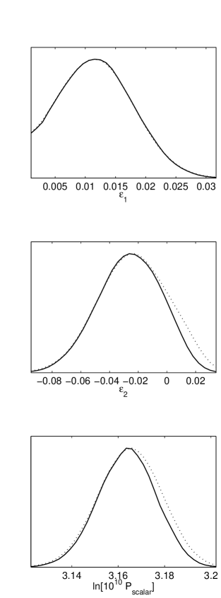
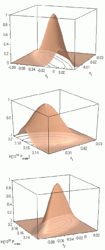
Figure 1: $1D$ marginalized probabilities (solid curve) and normalized mean likelihoods (dashed curve) for the slow-roll parameters $\epsilon_{{}_{1}}$, $\epsilon_{{}_{2}}$ and the scalar amplitude $P_{\mathrm{scalar}}$, in the case of the reference model. The three-dimensional plots show the normalized mean likelihoods and the corresponding $1\sigma$ and $2\sigma$ contours of the $2D$ marginalized probabilities.

The case of the last oscillatory parameter, i.e. the frequency, should be treated with great care. The frequency of the superimposed oscillations is given by $2\epsilon_{{}_{1}}/\sigma_{{}_{0}}$ and, hence, we have chosen to sample the quantity $\log\left(1/\sigma_{{}_{0}}\right)$. At this point, it is necessary to clarify what we exactly mean by “superimposed oscillations”. Indeed, if the frequency is very low and is such that less than half of a period covers the whole observable range of multipoles, then the resulting effect is just a modification of the overall amplitude of the power spectra and we don’t really have oscillations in the multipole moments anymore. In this regime, there is a strong degeneracy between the amplitude and $P_{\mathrm{scalar}}$. Clearly, it is not desirable to reach this extreme case. Another regime corresponds to the case where the frequency of the superimposed oscillations is of the same order of magnitude than the frequency of the acoustic oscillations. In this situation, new peaks would appear in the $C_{\ell}$’s and this could be problematic since the WMAP data are well described by the standard inflationary model. As a matter of fact, the amplitude of this type of oscillations is strongly constrained, see e.g. Ref. [28]. Finally, there is the case where high frequency oscillations are present. This is the case we are mostly interested in since it contains the improved fits found in Refs. [1, 2]. Nevertheless, very high values of the frequency lead to oscillations from multipole to multipole and any dependency on the frequency is in fact lost. It is clear that we would also like to avoid this extreme regime. All the above considerations has led us to restrict ourselves to $\log\left(1/\sigma_{{}_{0}}\right)\in[2.3,3.8]$ with a flat prior. This is equivalent to imposing a Jeffreys-like prior on $\sigma_{{}_{0}}$.

Our next step has been to generate Markov chains with COSMOMC for a standard slow-roll inflationary model without oscillation (i.e. for our reference, or vanilla, model) as well as for an oscillatory model characterized by $\psi$, $|x|\sigma_{{}_{0}}$ and $\log(1/\sigma_{{}_{0}})$ with the above priors, both cases being investigated with the non-primordial cosmological parameters chosen before. The standard inflationary model can be used as a reference for the restricted framework of the “fast parameter space”. For the two models, the Markov chains have been started from widespread point in the initial parameter space and stopped when the posterior distributions no longer evolve significantly which corresponds to about $250000$ elements. The generalized Gelman and Rubin $R$-statistics implemented in COSMOMC  [51, 53] is found to be less than $5\%$ for the slow-roll parameters and equal to approximately $9\%$ for the oscillatory parameters. However, the phase $\psi$ remains unconstrained. Let us recall that the $R$-statistics gives, for each parameter, the ratio of the variance of the chain means to the mean of the chain variances. In other words, it quantifies the errors in the parameter distributions obtained from the Markov chains exploration.

3 Results

In Fig. 1, we have plotted the one dimensional marginalized probabilities and the normalized mean likelihoods for the slow-roll parameters and the scalar amplitude in the case of the reference model. Three-dimensional plots of the mean likelihoods, obtained by averaging with respect to one parameter, are also represented with the $1\sigma$ and $2\sigma$ contours of the two-dimensional marginalized probabilities which appear through the surface. These plots are obviously consistent with the previously derived constraints [52], except that fixing the cosmological parameters has made the likelihood isocontours slightly tighter.

In Fig. 2, we have plotted the $1D$ marginalized probabilities and the normalized mean likelihoods for the parameters of the oscillatory model. In Figs. 3 and 4, the $1\sigma$ and $2\sigma$ contours of the $2D$ marginalized probabilities and the normalized mean likelihoods are displayed. They have been plotted in various planes of parameters, the parameters pairs being chosen to be the most correlated ones.

Let us now discuss the constraints that can be put on the amplitude of the oscillations, $|x|\sigma_{{}_{0}}$. As can be seen in Fig. 2, the vanilla slow-roll model, corresponding to $|x|\sigma_{{}_{0}}=0$, remains the most probable one with the currently available WMAP data. From the probability distribution, one finds that the $2\sigma$ marginalized upper limit is given by

$$|x|\sigma_{{}_{0}} <0.11\,.$$ (2)

However, the most striking feature of Fig. 2 is that the corresponding mean likelihood does not behave similarly to the marginalized probability, as it is the case for the other parameters. Indeed, it exhibits a maximum around $|x|\sigma_{{}_{0}}\simeq 0.1$ which is consistent with the best fits found in Refs. [1, 2]. This unusual behavior is expected if volume effects are present (more precisely, since we are dealing with quantities defined as integrals over the parameter space, the volume effects are important when the corresponding kernels are spread over this space with large values). This highlights the existence of strong non-linear correlations between $|x|\sigma_{{}_{0}}$ and the other parameters.

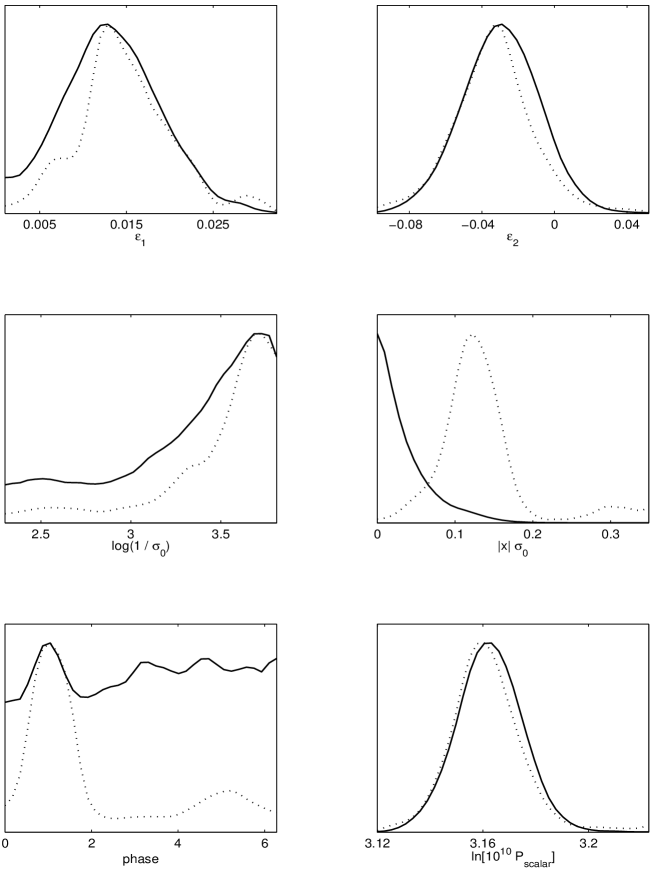
Figure 2: $1D$ marginalized probabilities (solid curves) and normalized mean likelihoods (dashed curves) for the oscillatory model.

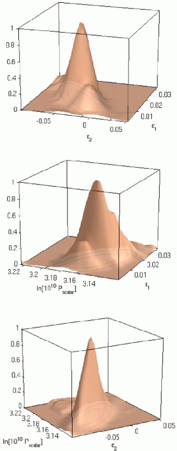
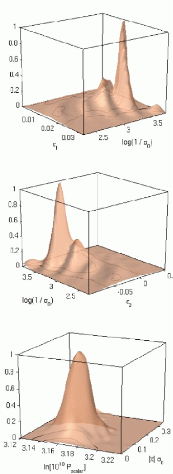
Figure 3: $1\sigma$ and $2\sigma$ contours of the $2D$ marginalized probabilities and normalized mean likelihoods (see also Fig. 4).

As can be seen in Fig. 4, strong correlations appear between the amplitude and the frequency of the oscillations. On the three-dimensional plot $\left[|x|\sigma_{{}_{0}},\log\left(1/\sigma_{{}_{0}}\right)\right]$, one remarks that the mean likelihood is non-vanishing either for large values of $\log\left(1/\sigma_{{}_{0}}\right)$, when $|x|\sigma_{{}_{0}}\neq 0$, or in a “long thin tube” centered around $|x|\sigma_{{}_{0}}=0$, the amplitude of which being much smaller (recall that $\Delta\chi^{2}\simeq 10$ between these two models). This behavior is expected since any frequency is possible provided its amplitude is very small hence the “long thin tube” around $|x|\sigma_{{}_{0}}=0$. On the other hand, for large values of $\log\left(1/\sigma_{{}_{0}}\right)$, one recovers a peak which corresponds to the oscillations fitting the outliers at relatively small scales [1, 2]. The marginalized probability is peaked at $|x|\sigma_{{}_{0}}=0$ because the tube has a bigger statistical weight, i.e. occupies a larger volume in the parameter space. Note also that this is the very existence of the likelihood peak at large $\log\left(1/\sigma_{{}_{0}}\right)$ which explains the long tail of the $1D$ marginalized probabilities for $|x|\sigma_{{}_{0}}$.

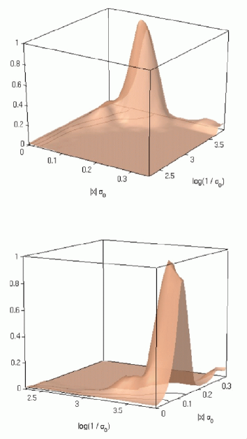
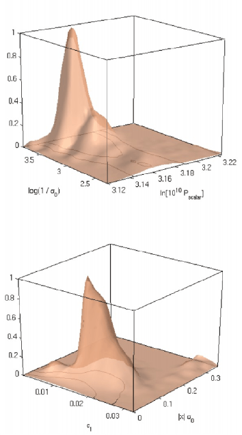
Figure 4: $1\sigma$ and $2\sigma$ contours of the $2D$ marginalized probabilities and normalized mean likelihoods (see also Fig. 3). Strong correlations appear between the amplitude and the frequency of the oscillations (on the left).

On the three-dimensional plot $\left[\epsilon_{{}_{1}},\log\left(1/\sigma_{{}_{0}}\right)\right]$, the wavelets in the mean likelihood originates from the degeneracy existing between $\sigma_{{}_{0}}$ and $\epsilon_{{}_{1}}$, for a fixed value of the frequency $2\epsilon_{{}_{1}}/\sigma_{{}_{0}}$. Furthermore, the correlation between $\epsilon_{{}_{1}}$ and $\epsilon_{{}_{2}}$ [52] is still present and, as a consequence, a correlation between $\epsilon_{{}_{2}}$ and $\log\left(1/\sigma_{{}_{0}}\right)$ also exists. We also remark that the correlations appearing when the oscillatory parameters are taken into account in the analysis seem to slightly tighten the confidence contours on the standard inflationary parameters and to cause the appearance of some multimodal features.

Another interesting property concerns the parameter $\log\left(1/\sigma_{{}_{0}}\right)$. As can be seen in Figs. 2, 3 and 4, both the mean likelihood and the marginalized probability are peaked at a high value of $\log\left(1/\sigma_{{}_{0}}\right)$. Quantitatively, a $1\sigma$ constraint on the energy scale $M_{\mathrm{c}}$ at which the new physics shows up can be derived

$$\sigma_{{}_{0}} \equiv{\textstyle\frac{\displaystyle H}{\displaystyle M_{\mathrm{c}}}}<6.6\times 10^{-4}\,.$$ (3)

Let us stress that this constraint is valid only if the amplitude and the frequency of the superimposed oscillations are considered as independent parameters. Indeed, it mainly comes from the region where the likelihood is strongly peaked and, as already noticed, this region does not exist if the parameter $x$ is chosen such that $x=1$. In this case, the likelihood is rather flat and, as a consequence, one would obtain a weaker contraint on the ratio $H/M_{\mathrm{c}}$.

Finally, we have found that the phase $\psi$ is not constrained as is clear from Fig. 2.

To end this section, one can ask how well the oscillatory model fits the data on average, compared to the standard slow-roll one. This can be estimated by comparing the mean likelihood over all the parameters in each of these models [51]. For the reference model one gets $\ln\bar{\mathcal{L}}_{\mathrm{sr}}\simeq-715.1$ while the oscillatory model has $\ln\bar{\mathcal{L}}_{\mathrm{wig}}\simeq-712.9$, hence a ratio of $\exp\left(715.1-712.9\right)\simeq 9$ in favor of the oscillatory model. This shows that including the oscillatory parameters permits to improve the goodness of fit on average [51].

4 Discussion and Conclusion

In this paper, we have explored, by means of Monte Carlo methods, the fast parameter space of an inflationary model with superimposed oscillations. This restricted framework is, at the time of writing, the only way to derive constraints in a reasonable computational time if the region where high frequency oscillations that better fit the CMB anisotropies outliers at relatively small scales [1, 2] is included. Among the main results derived in the present article are two constraints, one on the amplitude, $|x|\sigma_{{}_{0}}<0.11$, and the other of the energy scale $M_{\mathrm{c}}$, $H/M_{\mathrm{c}}<6.6\times 10^{-4}$.

The overall situation is quite interesting: on one hand, the fact that the marginalized probability is peaked at a value corresponding to a vanishing amplitude shows that the most probable model remains the standard slow-roll one for which $|x|\sigma_{{}_{0}}=0$. On the other hand, this distribution exhibits a long tail in the regions corresponding to non-vanishing amplitudes of the oscillations, precisely where the mean likelihood function is peaked, i.e. around $|x|\sigma_{{}_{0}}\simeq 0.1$. Moreover, the ratio of the vanilla slow-roll model to the oscillatory model total mean likelihoods is about $9$, in favor of the oscillatory model. This shows that, on average, the oscillatory model fits better the first year WMAP data.

The interpretation of the situation described above is as follows. The marginalized probabilities are quantities which are especially sensitive to “volume effects”, i.e. to the shape of the likelihood in regions of the parameter space where this one is significant. On the other hand, the mean likelihood is sensitive to the absolute value of the likelihood regardless to its occupied “volume”. Therefore, if in the parameter space there are regions which, at the same time, correspond to good fits and occupy a quite confined volume, then these regions will appear particularly significant from the mean likelihood point of view but will be “diluted” and, hence, will appear less significant from the marginalized probabilities point of view. Ultimately, the marginalized probability is the relevant quantity, that is to say is the quantity which should be used in order to conclude about the statistical meaning of a given model [54]. It will be interesting to study how the situation evolves when better data become available, in particular it will be interesting to see if the models with oscillations can occupy a volume which makes them probable from the marginalized probabilities point of view. This is one of the reasons why the next WMAP data release will be of great interest.

References

References

- [1] J. Martin and C. Ringeval, Superimposed oscillations in the wmap data?, Phys. Rev. D69 (2004) 083515, [astro-ph/0310382].
- [2] J. Martin and C. Ringeval, Addendum to “superimposed oscillations in the wmap data?”, Phys. Rev. D69 (2004) 127303, [astro-ph/0402609].
- [3] J. Martin and R. H. Brandenberger, The trans-planckian problem of inflationary cosmology, Phys. Rev. D63 (2001) 123501, [hep-th/0005209].
- [4] R. H. Brandenberger and J. Martin, The robustness of inflation to changes in super-planck- scale physics, Mod. Phys. Lett. A16 (2001) 999–1006, [astro-ph/0005432].
- [5] J. C. Niemeyer, Inflation with a high frequency cutoff, Phys. Rev. D63 (2001) 123502, [astro-ph/0005533].
- [6] A. Kempf, Mode generating mechanism in inflation with cutoff, Phys. Rev. D63 (2001) 083514, [astro-ph/0009209].
- [7] A. Kempf and J. C. Niemeyer, Perturbation spectrum in inflation with cutoff, Phys. Rev. D64 (2001) 103501, [astro-ph/0103225].
- [8] R. Easther, B. R. Greene, W. H. Kinney, and G. Shiu, Inflation as a probe of short distance physics, Phys. Rev. D64 (2001) 103502, [hep-th/0104102].
- [9] M. Lemoine, M. Lubo, J. Martin, and J.-P. Uzan, The stress-energy tensor for trans-planckian cosmology, Phys. Rev. D65 (2002) 023510, [hep-th/0109128].
- [10] L. Hui and W. H. Kinney, Short distance physics and the consistency relation for scalar and tensor fluctuations in the inflationary universe, Phys. Rev. D65 (2002) 103507, [astro-ph/0109107].
- [11] R. Easther, B. R. Greene, W. H. Kinney, and G. Shiu, Imprints of short distance physics on inflationary cosmology, Phys. Rev. D67 (2003) 063508, [hep-th/0110226].
- [12] J. C. Niemeyer and R. Parentani, Trans-planckian dispersion and scale-invariance of inflationary perturbations, Phys. Rev. D64 (2001) 101301, [astro-ph/0101451].
- [13] F. Lizzi, G. Mangano, G. Miele, and M. Peloso, Cosmological perturbations and short distance physics from noncommutative geometry, JHEP 06 (2002) 049, [hep-th/0203099].
- [14] U. H. Danielsson, A note on inflation and transplanckian physics, Phys. Rev. D66 (2002) 023511, [hep-th/0203198].
- [15] S. F. Hassan and M. S. Sloth, Trans-planckian effects in inflationary cosmology and the modified uncertainty principle, Nucl. Phys. B674 (2003) 434–458, [hep-th/0204110].
- [16] R. Easther, B. R. Greene, W. H. Kinney, and G. Shiu, A generic estimate of trans-planckian modifications to the primordial power spectrum in inflation, Phys. Rev. D66 (2002) 023518, [hep-th/0204129].
- [17] J. C. Niemeyer, R. Parentani, and D. Campo, Minimal modifications of the primordial power spectrum from an adiabatic short distance cutoff, Phys. Rev. D66 (2002) 083510, [hep-th/0206149].
- [18] N. Kaloper, M. Kleban, A. Lawrence, S. Shenker, and L. Susskind, Initial conditions for inflation, JHEP 11 (2002) 037, [hep-th/0209231].
- [19] L. Bergstrom and U. H. Danielsson, Can map and planck map planck physics?, JHEP 12 (2002) 038, [hep-th/0211006].
- [20] K. Goldstein and D. A. Lowe, A note on alpha-vacua and interacting field theory in de sitter space, Nucl. Phys. B669 (2003) 325–340, [hep-th/0302050].
- [21] G. L. Alberghi, R. Casadio, and A. Tronconi, Trans-planckian footprints in inflationary cosmology, Phys. Lett. B579 (2004) 1–5, [gr-qc/0303035].
- [22] C. Armendariz-Picon and E. A. Lim, Vacuum choices and the predictions of inflation, JCAP 0312 (2003) 006, [hep-th/0303103].
- [23] J. Martin and R. Brandenberger, On the dependence of the spectra of fluctuations in inflationary cosmology on trans-planckian physics, Phys. Rev. D68 (2003) 063513, [hep-th/0305161].
- [24] H. Collins, R. Holman, and M. R. Martin, The fate of the alpha-vacuum, Phys. Rev. D68 (2003) 124012, [hep-th/0306028].
- [25] O. Elgaroy and S. Hannestad, Can planck-scale physics be seen in the cosmic microwave background?, Phys. Rev. D68 (2003) 123513, [astro-ph/0307011].
- [26] N. Kaloper and M. Kaplinghat, Primeval corrections to the cmb anisotropies, Phys. Rev. D68 (2003) 123522, [hep-th/0307016].
- [27] H. Collins and R. Holman, Taming the alpha vacuum, Phys. Rev. D70 (2004) 084019, [hep-th/0312143].
- [28] T. Okamoto and E. A. Lim, Constraining cut-off physics in the cosmic microwave background, Phys. Rev. D69 (2004) 083519, [astro-ph/0312284].
- [29] A. Ashoorioon, A. Kempf, and R. B. Mann, Minimum length cutoff in inflation and uniqueness of the action, astro-ph/0410139.
- [30] R. H. Brandenberger and J. Martin, Back-reaction and the trans-planckian problem of inflation revisited, hep-th/0410223.
- [31] U. H. Danielsson, Transplanckian energy production and slow roll inflation, hep-th/0411172.
- [32] B. R. Greene, K. Schalm, G. Shiu, and J. P. van der Schaar, Decoupling in an expanding universe: Backreaction barely constrains short distance effects in the cmb, hep-th/0411217.
- [33] J. Barriga, E. Gaztanaga, M. G. Santos, and S. Sarkar, On the apm power spectrum and the cmb anisotropy: Evidence for a phase transition during inflation?, Mon. Not. Roy. Astron. Soc. 324 (2001) 977, [astro-ph/0011398].
- [34] X. Wang, B. Feng, and M. Li, Natural inflation, planck scale physics and oscillating primordial spectrum, astro-ph/0209242.
- [35] C. P. Burgess, J. M. Cline, F. Lemieux, and R. Holman, Are inflationary predictions sensitive to very high energy physics?, JHEP 02 (2003) 048, [hep-th/0210233].
- [36] J. Martin and P. Peter, Parametric amplification of metric fluctuations through a bouncing phase, Phys. Rev. D68 (2003) 103517, [hep-th/0307077].
- [37] J. Martin and P. Peter, On the ’causality argument’ in bouncing cosmologies, Phys. Rev. Lett. 92 (2004) 061301, [astro-ph/0312488].
- [38] P. Hunt and S. Sarkar, Multiple inflation and the wmap ’glitches’, Phys. Rev. D70 (2004) 103518, [astro-ph/0408138].
- [39] H. V. Peiris et. al., First year wilkinson microwave anisotropy probe (wmap) observations: Implications for inflation, Astrophys. J. Suppl. 148 (2003) 213, [astro-ph/0302225].
- [40] C. L. Bennett et. al., First year wilkinson microwave anisotropy probe (wmap) observations: Preliminary maps and basic results, Astrophys. J. Suppl. 148 (2003) 1, [astro-ph/0302207].
- [41] G. Hinshaw et. al., First year wilkinson microwave anisotropy probe (wmap) observations: Angular power spectrum, Astrophys. J. Suppl. 148 (2003) 135, [astro-ph/0302217].
- [42] L. Verde et. al., First year wilkinson microwave anisotropy probe (wmap) observations: Parameter estimation methodology, Astrophys. J. Suppl. 148 (2003) 195, [astro-ph/0302218].
- [43] A. Kogut et. al., Wilkinson microwave anisotropy probe (wmap) first year observations: Te polarization, Astrophys. J. Suppl. 148 (2003) 161, [astro-ph/0302213].
- [44] N. Kogo, M. Matsumiya, M. Sasaki, and J. Yokoyama, Reconstructing the primordial spectrum from wmap data by the cosmic inversion method, Astrophys. J. 607 (2004) 32–39, [astro-ph/0309662].
- [45] A. Shafieloo and T. Souradeep, Primordial power spectrum from wmap, Phys. Rev. D70 (2004) 043523, [astro-ph/0312174].
- [46] A. Lewis, A. Challinor, and A. Lasenby, Efficient computation of cmb anisotropies in closed frw models, Astrophys. J. 538 (2000) 473–476, [astro-ph/9911177].
- [47] J. Martin and D. J. Schwarz, The influence of cosmological transitions on the evolution of density perturbations, Phys. Rev. D57 (1998) 3302–3316, [gr-qc/9704049].
- [48] J. Martin and D. J. Schwarz, The precision of slow-roll predictions for the cmbr anisotropies, Phys. Rev. D62 (2000) 103520, [astro-ph/9911225].
- [49] J. Martin, A. Riazuelo, and D. J. Schwarz, Slow-roll inflation and cmb anisotropy data, Astrophys. J. 543 (2000) L99–L102, [astro-ph/0006392].
- [50] D. J. Schwarz, C. A. Terrero-Escalante, and A. A. Garcia, Higher order corrections to primordial spectra from cosmological inflation, Phys. Lett. B517 (2001) 243–249, [astro-ph/0106020].
- [51] A. Lewis and S. Bridle, Cosmological parameters from cmb and other data: a monte- carlo approach, Phys. Rev. D66 (2002) 103511, [astro-ph/0205436].
- [52] S. M. Leach and A. R. Liddle, Constraining slow-roll inflation with wmap and 2df, Phys. Rev. D68 (2003) 123508, [astro-ph/0306305].
- [53] S. P. Brooks and A. Gelman J. Comp. Graph. Stat. 7 (1998) 434.
- [54] M. Aitkin J. Roy. Statist. Soc. B53 (1991) 111.