B=2 Oblate Skyrmions

Abstract

The numerical solution for the $B=2$ static soliton of the $SU(2)$ Skyrme model shows a profile function dependence which is not exactly radial. We propose to quantify this with the introduction of an axially symmetric oblate ansatz parametrized by a scale factor $d.$ We then obtain a relatively deformed bound soliton configuration with $M_{B=2}/M_{B=1}=1.958$. This is the first step towards to description of $B>1$ quantized states such as the deuteron with a non-rigid oblate ansatz where deformations due to centrifugal effects are expected to be more important.

year number number identifier LABEL:FirstPage1 LABEL:LastPage#1

I

II INTRODUCTION

The Skyrme model Skyrme is a nonlinear effective field theory of weakly coupled pions in which baryons emerge as localized finite energy soliton solutions. The stability of such solitons is guaranteed by the existence of a conserved topological charge interpreted as the quantum baryon number $B$. More specifically, Skyrmions consist in static pion field configurations which minimize the energy functional of the Skyrme model in a given nontrivial topological sector. The model is partly motivated by the large-$N_{c}$ QCD analysis t'Hooft ; Witten , as there are reasons to believe that once properly quantized, a refined version of the model could accurately depict nucleons as well as heavier atomic nuclei with mesonic degrees of freedom Braaten ; Houghton ; Scoccola in the low energy limit.

In the lowest nontrivial topological sector $B=1$, the Skyrmion is described by the spherically symmetric hedgehog ansatz which reproduces experimental data with an accuracy of $30\%$ or better Adkins . However, this relative success radically contrasts with the situation encountered in the $B>2$ sector, where the hedgehog ansatz is not the lowest energy configuration and would not give rise to bound state configurations Jackson ; Weigel . Moreover, pioneering numerical investigations of Verbaarschot Verbaarschot clearly indicate that the $B=2$ Skyrmion is not spherically symmetric, but rather possesses an axial symmetry reflected in its doughnut-like baryon density. Further inspection of this numerical solution, in particular the profile function, suggests that the classical biskyrmion may be represented by an oblate field configuration. Yet, most of the trial functions used to describe such a solution assume a decoupling from the angular degrees of freedom, i.e. $F(r,\theta,\phi)=F(r)$, as this is the case for the instanton-inspired ansatz proposed in Atiyah or in the early variational approach Thomas ; Kurihara for example. On the other hand, some axially symmetric solutions were analysed in the $B=1$ sector, by Hajduk and Marleau respectively, to include possible deformations due to centrifugal effects undergone by the rotating Skyrmion and account for the quadrupole deformations of baryons. Here, our aim is to extend the work on oblate Skyrmions in Marleau to describe dibaryon states. The classical static oblate solution introduced in this manner will provide a quantitative estimate of the axial deformation, which is different from a uniform scaling in a given direction as performed in Hajduk . It should also provide an adequate ground to perform the quantization of the $B=2$ soliton.

There has been several attempts to decribed the angular dependence of the $B>1$ solutions which is much more complicated than the hedgehog form in $B=1.$ Fortunately, a few years ago, Houghton et al. Houghton came up with an interesting ansatz based on rational maps. The rational map ansatz provides a simple alternative compared to the full numerical study of the angular dependence of the baryon density distribution of multiskyrmions. It also yields static energy predictions in good agreement with numerical solutions for several values of $B$. The most interesting feature of this method remains without doubt that fundamental symmetries of multiskyrmions can easily be implemented in the ansatz solutions. This provides a clever way to identify the symmetries of the exact solutions, which are not always apparent, and in some cases, adequate initial solutions for lengthy numerical calculations. Close as it may be, the rational map ansatz remains an approximation and in some cases, more accurate angular ansatz have been found. For example, Houghton and Krusch Houghton2 slightly improved the mass approximation of the biskyrmion by relaxing the requirement of holomorphicity imposed on rational maps. However, the profile function defined in this work still solely depends on $r$. As may seems evident, some accuracy still may be gained by introducing a more appropriate parametrization of the soliton shape function. Recently, Ioannidou et al. Ioannidou obtained similar results by introducing an improved harmonic maps ansatz where the profile function depends on radial and polar degrees of freedom as well. However, they had to deal with a complicated second-order partial differential equation.

From these considerations, we propose a $B=2$ oblate solution based on rational maps, which could be understood as the rational maps solution proposed in Houghton ; Krusch with the radial dependence $F(r)$ replaced by an oblate form $f(\eta)$. Consequently, the soliton undergoes a smoothly flattening along a given axis of symmetry. The parameter $d$ provides a measure of the scale at wich the deformation becomes important while the solution preserves the angular dependence given by the rational maps scheme for the $B=2$ case. This choice is obviously consistent with the toroidal baryon density of the $B=2$ Skyrmion. Implementing the oblate ansatz to the model, we first integrate analytically the angular degrees of freedom. This explains why other angular ansatz such as those in Houghton2 and Ioannidou were not chosen; they led to complications. The second step involve solving the remaining nonlinear ordinary second-order differential equation resulting from the minimization of the static energy functional with respect to the profile function $f(\eta)$. Thereby, the parameter $d$ is set as to minimize the static energy, i.e. the mass of the soliton. Although the method applies to higher baryon numbers and other Skyrme model extensions, the analysis is restricted here to $B=2$ Skyrmion for $SU(2)$ Skyrme model.

In the next section, we present the axially symmetric oblate ansatz for the SU(2) Skyrme model introducing the oblate spheroidal coordinates. In section III, we briefly describe rational maps and show how they can be used in the context of static oblate biskyrmions. A discussion of the numerical results follows in the last section, where we also draw concluding remarks about how the oblate-like solution could be a good starting point to perform the quantization of the non-rigid $B=2$ soliton as the deuteron.

III STATIC OBLATE MULTISKYRMIONS

Let us first introduce the oblate spheroidal coordinates $(\eta,\theta,\phi),$ which are related to Cartesian coordinates through

$$(x,y,z)=d(\cosh\eta\sin\theta\cos\phi,\cosh\eta\sin\theta\sin\phi,\sinh\eta\cos\theta),$$ (1)

so a surface of constant $\eta$ correspond to a sphere of radius $d\cosh\eta$ flattened in the $z$-direction by a factor of $\tanh\eta$. For small $\eta$, these surfaces are quite similar to that of pancakes of radius $d$ whereas when $\eta$ is large, they become spherical shells of radius given by $(d/2)e^{\eta}$. Note that taking the double limit $d\rightarrow 0,\eta\rightarrow\infty$ such that $r$ always remains finite, one recovers the usual spherical coordinates. Thus, the choice of the parameter $d$ establishes the scale at which the oblateness becomes significant. Finally, the element of volume reads

$$dV=-d^{3}\cosh\eta\left(\sinh^{2}\eta+\cos^{2}\theta\right)d\eta\ d(\cos\theta)\ d\phi.$$ (2)

Neglecting the pion mass term, the chirally invariant Lagrangian of the $SU(2)$ Skyrme model just reads

$${\mathcal{L}}=-\frac{F_{\pi}^{2}}{16}\operatorname*{Tr}L_{\mu}L^{\mu}+\frac{1}{32e^{2}}\operatorname*{Tr}[L_{\mu},L_{\nu}]^{2}$$ (3)

where $L_{\mu}=U^{\dagger}\partial_{\mu}U$ with $U\in SU(2)$. Here, $F_{\pi}$ is the pion decay constant and $e$ is sometimes referred to as the Skyrme parameter. In order to implement an oblate solution, let us now replace the hedgehog ansatz

$$U=e^{i\mathbf{\tau}\ \cdot\ \mathbf{\widehat{r}}\ F(r)}$$ (4)

by the static oblate solution defined as follow

$$U=e^{i\mathbf{\tau}\ \cdot\ \mathbf{\widehat{\eta}}\ f(\eta)}$$ (5)

where the ${\tau}_{k}$ stand for the Pauli matrices while ${\widehat{\eta}}$ is the standard unit vector ${\widehat{\eta}}={\vec{\nabla}\eta}/{|\vec{\nabla}\eta|}$. More explicitly, this unit vector is simply

$${\widehat{\eta}}=\frac{(\cosh\eta\sin\Theta\cos\Phi,\cosh\eta\sin\Theta\sin\Phi,\sinh\eta\cos\Theta)}{\sqrt{\cosh^{2}\eta-\cos^{2}\Theta)}},$$ (6)

As will become apparent in the next section, we consider the case where $\Theta\equiv\Theta(\theta)$ and $\Phi\equiv\Phi(\phi),$ i.e. $\Theta$ and $\Phi$ depend only on the polar angle $\theta$ and the azimuthal angle $\phi$ respectively. Furthermore, $f(\eta)$, which determines the global shape of the soliton, plays the role of the so-called profile function. In that respect, the oblate ansatz is clearly different from a scale transformation along one of the axis Hajduk . As in its original hedgehog form, the field configuration $U$ constitutes a map from the physical space ${\mathcal{R}}^{3}$ onto the Lie group manifold of $SU(2)$. Finite energy solutions require that this $SU(2)$ valued field goes to the trivial vacuum for asymptotically large distances, that is $U(\eta\rightarrow\infty)\rightarrow 1_{2\times 2}$.

The expression for the static energy density is

$${\mathcal{E}}={\mathcal{E}}_{2}+{\mathcal{E}}_{4}=-\frac{F_{\pi}^{2}}{16}Tr(L_{i}L_{i})+\frac{1}{32e^{2}}Tr\left([L_{i},L_{j}]^{2}\right)$$ (7)

so, after substituting the oblate ansatz, the mass functional can be written as

$$M[f(\eta),\Theta(\theta),\Phi(\phi)]=\int dV\left({\mathcal{M}}_{2}+{\mathcal{M}}_{4}\right)$$ (8)

with

$${\mathcal{M}}_{2}=\frac{F_{\pi}^{2}}{8}\left(|\vec{\nabla}\eta|^{2}\ f^{\prime 2}+\sin^{2}f\ {\tilde{K}}\right)$$ (9)

and

$${\mathcal{M}}_{4}=\frac{1}{4e^{2}}\left(2|\vec{\nabla}\eta|^{2}\ f^{\prime 2}\ {\tilde{K}}+\sin^{4}f\ \left({\tilde{K}}^{2}-{\tilde{K}}_{ab}{\tilde{K}}_{ab}\right)\right).$$ (10)

Here, the notation is lighten by the use of the ${\tilde{K}}_{ab}$ matrix defined as:

$${\tilde{K}}_{ab}=\vec{\nabla}_{i}\widehat{\eta}_{a}\vec{\nabla}_{i}\widehat{\eta}_{b}$$ (11)

$${\tilde{K}}=Tr({\tilde{K}}_{ab})={\tilde{K}}_{aa}.$$ (12)

Introducing an auxiliary variable for convenience,

$$\Sigma=\cos^{2}\Theta\ \sin^{2}\Theta+\Theta^{\prime 2}\ \cosh^{2}\eta\ \sinh^{2}\eta$$ (13)

one easily deduces that

$${\tilde{K}}=\left(\frac{|\vec{\nabla}\eta|^{2}\Sigma}{(\cosh^{2}\eta-\cos^{2}\Theta)^{2}}+\Phi^{\prime 2}\ \frac{(\sin^{2}\Theta/\sin^{2}\theta)}{d^{2}(\cosh^{2}\eta-\cos^{2}\Theta)}\ \right)$$ (14)

and

$${\tilde{K}}^{2}-{\tilde{K}}_{ab}{\tilde{K}}_{ab}=\frac{2}{d^{2}}\ \Phi^{\prime 2}\ \frac{|\vec{\nabla}\eta|^{2}\Sigma(\sin^{2}\Theta/\sin^{2}\theta)}{(\cosh^{2}\eta-\cos^{2}\Theta)^{3}}.$$ (15)

However, before minimizing the mass functional with respect to the chiral angle $f(\eta)$, in view to get the static configuration of the soliton, one must specify an angular dependence in $\Theta(\theta)$ and $\Phi(\phi)$. This is the subjet of the next section, after a brief recall of some basic features related to the rational maps ansatz.

IV OBLATE SKYRMIONS AND RATIONAL MAPS

Formally, a rational map of order $N$ consists in a ${\mathcal{S}}^{2}\rightarrow{\mathcal{S}}^{2}$ holomorphic map of the form

$$R_{N}(z)=\frac{p(z)}{q(z)}$$ (16)

where $p$ and $q$ appear as polynomials of degree at most $N$. Moreover, these maps are built in such a way that $p$ or $q$ is precisely of degree $N$. It is also assumed that $p$ and $q$ do not share any common factor. Any point $z$ on ${\mathcal{S}}^{2}$ is identified via stereographic projection, defined through $z=\tan(\frac{\theta}{2})\ e^{i\phi}$. Thus, the image of a rational map $R(z)$ applied on a point $z$ of a Riemann sphere corresponds to the unit vector

$$\widehat{n}_{R}=\frac{1}{1+|R_{N}|^{2}}\ \left(2\Re R_{N}(z),2\Im R_{N}(z),1-|R_{N}|^{2}\right)$$ (17)

which also belongs to a Riemann sphere. The link between static soliton chiral fields and rational maps Houghton follows from the ansatz

$$U_{R}(r,z)=e^{i\widehat{n}_{R}\cdot\vec{\tau}F(r)}$$ (18)

inasmuch as $F(r)$ acts as radial chiral angle function. To be well defined at the origin and at $r\rightarrow\infty$, the boundary conditions must be $F(0)=k\pi$ where $k$ is an integer and $F(\infty)=0.$ The baryon number is given by $B=Nk$ where $N=\max(\deg p,\deg q)$ is the degree of $R_{N}(z).$ We consider only the case $k=1$ here, so $B=N$.

By analogy with the nonlinear theory of elasticity Manton , Manton has showed that the static energy of Skyrmions could be understood as the local stretching induced by the map $U:{\mathcal{R}}^{3}\rightarrow{\mathcal{S}}^{3}$. In this real rubber-sheet geometry, the Jacobian $J$ of the transformation provides a basic measure of the local distortion caused by the map $U$. This enables us to build a symmetric positive definite strain tensor defined at every point of ${\mathcal{R}}^{3}$ as

$$D_{ij}=J_{i}J_{j}^{T}=-\frac{1}{2}Tr\left(L_{i}L_{j}\right).$$ (19)

This strain tensor $D$, changing into $O^{T}DO$ under orthogonal transformations, comes with three invariants expressed in terms of its eigenvalues $\lambda_{1}^{2}$, $\lambda_{2}^{2}$ and $\lambda_{3}^{2}$:

$$Tr\;D=\lambda_{1}^{2}+\lambda_{2}^{2}+\lambda_{3}^{2}$$ (20)

$$\frac{1}{2}(Tr\;D)^{2}-\frac{1}{2}Tr\;D^{2}=\lambda_{1}^{2}\lambda_{2}^{2}+\lambda_{2}^{2}\lambda_{3}^{2}+\lambda_{1}^{2}\lambda_{3}^{2}$$ (21)

$$det\;D=\lambda_{1}^{2}\lambda_{2}^{2}\lambda_{3}^{2}.$$ (22)

Since it is assumed that geometrical distorsion is unaffected by rotations of the coordinates frame in both space and isospace, the energy density should remain invariant and could be written as a function of the basic invariants as follows

$${\mathcal{E}}=\alpha\left(\lambda_{1}^{2}+\lambda_{2}^{2}+\lambda_{3}^{2}\right)+\beta\left(\lambda_{1}^{2}\lambda_{2}^{2}+\lambda_{2}^{2}\lambda_{3}^{2}+\lambda_{1}^{2}\lambda_{3}^{2}\right)$$ (23)

where $\alpha$ and $\beta$ are parameter depending on $F_{\pi}$ and $e,$ while the baryon density is associated with the quantity

$$B^{0}=\frac{\lambda_{1}\lambda_{2}\lambda_{3}}{2\pi^{2}}.$$ (24)

In this picture, radial strains are orthogonal to angular ones. Moreover, owing to the conformal aspect of $R_{N}(z)$, angular strains are isotropic. Thereby, it is customary to identify

$$\lambda_{1}=-F^{\prime}(r)$$ (25)

and

$$\lambda_{2}=\lambda_{3}=\frac{\sin F(r)}{r}\ \frac{1+|z|^{2}}{1+|R_{N}(z)|^{2}}\ \left|\frac{dR_{N}(z)}{dz}\right|\ .$$ (26)

Thus, substituting these eigenvalues in (23) and integrating over physical space yields

$$M_{N}=\int dr\left(\frac{\pi F_{\pi}^{2}}{2}\;{\mathcal{E}}_{2}^{N}+\frac{2\pi}{e^{2}}\;{\mathcal{E}}_{4}^{N}\right)$$ (27)

with

$${\mathcal{E}}_{2}^{N}=\left(F^{\prime 2}+2N\frac{\sin^{2}F}{r^{2}}\right)$$ (28)

$${\mathcal{E}}_{4}^{N}=\left(2NF^{\prime 2}\frac{\sin^{2}F}{r^{2}}+{\mathcal{I}}_{N}\frac{\sin^{4}F}{r^{2}}\right)$$ (29)

and

$${\mathcal{I}}_{N}=\frac{1}{4\pi}\int\frac{2idzd\bar{z}}{|1+|z|^{2}|^{2}}\ \left(\frac{1+|z|^{2}}{1+|R_{N}(z)|^{2}}\left|\frac{dR_{N}(z)}{dz}\right|\right)^{4},$$ (30)

wherein $\frac{2idzd\bar{z}}{|1+|z|^{2}|^{2}}$ corresponds to the usual area element on a 2-sphere, that is $\sin\theta\ d\theta\ d\phi$. At first glance, one sees that radial and angular contributions to the static energy are clearly singled out.

Now, focussing on the $N=2$ case, the most general rational map reads

$$R_{2}(z)=\frac{\alpha z^{2}+\beta z+\gamma}{\mu z^{2}+\nu z+\lambda}.$$ (31)

However, imposing the exact $2-$torus symmetries (axial symmetry and rotations of $180^{o}$ around Cartesian axes), as expected from numerical analysis Verbaarschot , restricts the general form above to this one

$$R_{2}(z)=\frac{z^{2}-a}{-az^{2}+1}.$$ (32)

It has been showed in Houghton that ${\mathcal{I}}_{2}$, and thus the mass functional alike, exhibits a minimum for $a=0$. Then, one must conclude that the most adequate choice of a rational map for the description of the biskyrmion solution boils down to $R_{2}(z)=z^{2}$. Recasting this map in term of angular variables $(\theta,\phi)\rightarrow(\Theta,\Phi)$, we get

$$z \rightarrow R_{2}(z)=\tan(\frac{\Theta}{2})\ e^{i\Phi}=\tan^{2}(\frac{\theta}{2})\ e^{2i\phi}$$

$$\theta \rightarrow\Theta(\theta)=\arcsin\left(\frac{\sin^{2}\theta}{1+\cos^{2}\theta}\right)$$

$$\phi \rightarrow\Phi(\phi)=2\phi$$

It is easy to verify that for $B=1,$ the rational map is simply $R(z)=z,$ or $\Theta(\theta)=\theta$ and $\Phi(\phi)=\phi$, and one recovers the energy density in Houghton .

We shall assume here that this angular function still holds in the oblate picture in (9-15). After analytical angular integrations are performed, the mass of the oblate biskyrmion can be cast in the form

$$M=\frac{4\pi\epsilon}{\lambda}\int_{0}^{\infty}d\eta\left(\frac{\tilde{d}}{2}\;{\mathcal{E}}_{2}+\frac{1}{4\tilde{d}}\;{\mathcal{E}}_{4}\right)$$ (33)

with

$${\mathcal{E}}_{2}={\mathcal{M}}_{21}f^{\prime 2}+{\mathcal{M}}_{22}\sin^{2}f$$ (34)

and

$${\mathcal{E}}_{4}={\mathcal{M}}_{41}f^{\prime 2}\sin^{2}f+{\mathcal{M}}_{42}\sin^{4}f.$$ (35)

The explicit expressions of the density functions ${\mathcal{M}}_{ij}(\eta)$, which are reported in Appendix A, follow from straightforward but tedious calculations. Adopting the same conventions as in Marleau , for the sake of comparison, we also rescaled the deformation parameter as ${\tilde{d}}=eF_{\pi}d/2\sqrt{2}$, with $\epsilon=1/\sqrt{2}e$ and $\lambda=2/{F_{\pi}}$. The values of $F_{\pi}=129$ MeV and $e=5.45$ are chosen to coincide with those of Adkins . Now, the chiral angle function $f(\eta)$ can be determined from the minimization of the above functional, i.e. requiring that $\delta M[f(\eta)]=0$ . Thus static field configuration must obey the following nonlinear second-order ODE:

$$0 =f^{\prime\prime}\left(2\tilde{d}\cosh\eta+\frac{1}{2\tilde{d}}{\mathcal{M}}_{41}\sin^{2}f\right)+f^{\prime 2}\left(\frac{1}{2\tilde{d}}{\mathcal{M}}_{41}\sin f\cos f\right)$$

$$+f^{\prime}\left(2\tilde{d}\sinh\eta+\frac{1}{2\tilde{d}}{\mathcal{M}}_{41}^{\prime}\sin^{2}f\right)$$

$$-\tilde{d}{\mathcal{M}}_{22}\sin f\cos f-\frac{1}{\tilde{d}}{\mathcal{M}}_{42}\sin^{3}f\cos f\quad.$$ (36)

Here, the primes merely denote derivatives with respect to $\eta$. Solving numerically for several values of $\tilde{d}$, we obtain the set of chiral angle functions of Figure 1. When $\tilde{d}$ is small, we recover exactly the solution of the $N=2$ rational map ansatz. Let us stress that increasing $\tilde{d}$ enforces a continuous displacement of the function $f(\eta)$ which induces a smooth deformation of the soliton.

Figure 1: Oblate biskyrmion chiral angle for several values of $\tilde{d}$. From left to right, we have $\tilde{d}=$ 0.5, 0.2,0.1, 0.05, 0.01, 0.005 and 0.001.

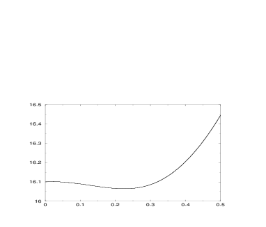
Figure 2: The mass of the oblate biskyrmion solution as a function of $\tilde{d}$. The mass reaches its minimal value for $\tilde{d}=0.225$.

In Figure 2, we plot the mass of the oblate biskyrmion as a function of $\tilde{d}$. The mass of the biskyrmion passes trough a minimum for a finite non-zero value of the parameter $\tilde{d}$. This is a clear indication that the oblate solution is energically favored. Note again that in the limit $\tilde{d}\rightarrow 0$, we reproduce the mass value found in Houghton ; Krusch with the rational maps ansatz and profile function with radial dependence $F(r)$.

V NUMERICAL RESULTS AND DISCUSSION

Numerical calculations carried out some years ago by Verbaarschot Verbaarschot and almost concurrently by Kopeliovich and Stern Kopeliovich , establish that in the Skyrme model the mass ratio $R_{2/1}=M_{B=2}/M_{B=1}$ is $1.92$. The $B=2$ oblate solution also represents a bound state of two solitons since its mass is lower than twice the mass found in the $B=1$ sector Marleau . From our calculations, we get that the mass of the static oblate biskyrmion, being minimized for $\tilde{d}=0.225$, is $16.066\frac{4\pi\epsilon}{\lambda}$ or $1689.5$ MeV. The parameter $\tilde{d}=0.225$ provides a measure of how the the $B=2$ solution is flattened. Hence, the mass ratio of our flattened solution turns out to be $R_{2/1}=1.958$. Comparing to other ansatz for $B=2$  solutions, it is fairly smaller than that predicted by the familiar hedgehog ansatz with boundary conditions $F(0)=2\pi$ and $F(\infty)=0$, since then $R_{2/1}>3$ Jackson or and still better than the hedgehog-like solution with $\phi\rightarrow 2\phi$ proposed as in Weigel , whose mass ratio is $R_{2/1}=2.14$ . Note that none of these solutions are stable solutions since $R_{2/1}>2$. Let us mention that Kurihara et al. Kurihara achieved a mass ratio of $1.94$ using a different angular parametrization. However, there are no obvious physical grounds for their angular trial function and it remains that rational maps are far more superior when it comes to depict the symmetries of the $B>1$ solutions. Our results still represent a slight improvement over those obtained in the original framework of rational maps, i.e. $R_{2/1}=1.962$ Houghton , where the chiral angle is strictly radial. Hence the oblate solution which depends of a spheroidal oblate coordinate $\eta,$ captures more exactly the profile shape of the biskyrmion than the original rational maps ansatz does although both rely on rational maps. The relatively small improvement also suggests that a better ansatz for classical $B=2$ static solution would require a different choice for the angular dependence. In that regard, Houghton2 and Ioannidou both achieved a mass ratio of $1.933$ by dropping the constraint on the rational maps to be holomorphic. These alternatives remain very difficult to implement for an oblate field configuration.

It is worth emphasizing that the procedure presented here generalizes to any baryon number and any choice of angular ansatz consistent with multiskyrmions symmetries although analytical angular integration may become more cumbersome if not impossible in those cases. Similarly, the approach can be generalized to other Skyrme-like effective Lagrangians.

In this paper we only investigated the classical $B=2$ static solution but in principle, the full solution requires a quantization treatment to account for the quantum properties of dibaryons. The most standard procedure consists in a semiclassical quantization using collective variables. It only adds simple kinetic terms to the Hamiltonian but these energy contributions should partially fill the energy gap between the $(I=0,J=1)$ deuteron mass ($1876$ MeV) and that of our deformed $B=2$ static Skyrmion ($1689.5$ MeV). So, even if our analytical oblate ansatz is not necessarily the lowest static energy solution for the $B=2$ Skyrmion, the optimization of the oblateness parameter $\tilde{d}$ should prove adequate to take into account the soliton deformation due to centrifugal effects, as for the $B=1$ case Marleau . Thus, following such a procedure, we can expect that the properly quantized biskyrmion solution would provide a good starting point for the description of the low energy phenomenology of the deuteron Braaten ; Leese ; Riska . The problem of quantization of the oblate biskyrmion solution is an important topic in itself and will be addressed elsewhere.

VI ACKNOWLEDGEMENTS

J.-F. Rivard is indebted to H. Jirari for useful discussions on computational methods and numerical analysis. This work was supported in part by the Natural Sciences and Engineering Research Council of Canada.

VII APPENDIX

Performing angular integrations in the oblate static energy functional, we get the following ${\mathcal{M}}_{ij}(\eta)$ density functions:

$${\mathcal{M}}_{21}=2\cosh\eta$$

$${\mathcal{M}}_{22}=\frac{2\cosh^{2}\eta-7}{\cosh\eta}+\frac{\pi(8\cosh^{2}\eta-7)}{2\cosh^{2}\eta\sqrt{\cosh^{2}\eta-1}}+\frac{6\cosh^{4}\eta-11\cosh^{2}\eta+7}{2\cosh^{2}\eta}L(\eta)$$

$${\mathcal{M}}_{41} =\frac{L(\eta)\ \left(2\cosh^{12}\eta-15\cosh^{10}\eta+45\cosh^{8}\eta-86\cosh^{6}\eta+124\cosh^{4}\eta-92\cosh^{2}\eta+24\right)}{2(\cosh^{6}\eta-4\cosh^{4}\eta+8\cosh^{2}\eta-4)^{2}}$$

$$-\frac{\pi\ \left(8\cosh^{10}\eta-53\cosh^{8}\eta+120\cosh^{6}\eta-136\cosh^{4}\eta+76\cosh^{2}\eta-16\right)}{2\sqrt{\cosh^{2}\eta-1}\ (\cosh^{6}\eta-4\cosh^{4}\eta+8\cosh^{2}\eta-4)^{2}}$$

$$+\frac{8\cosh^{5}\eta\ \arctan\left(\frac{1}{\sqrt{\cosh^{2}\eta-1}}\right)\ (\cosh^{6}\eta-5\cosh^{4}\eta+7\cosh^{2}\eta-3)}{\sqrt{\cosh^{2}\eta-1}\ (\cosh^{6}\eta-4\cosh^{4}\eta+8\cosh^{2}\eta-4)^{2}}$$

$$+\frac{(2\cosh^{11}\eta-11\cosh^{9}\eta+30\cosh^{7}\eta-40\cosh^{5}\eta+28\cosh^{3}\eta-8\cosh\eta)}{(\cosh^{6}\eta-4\cosh^{4}\eta+8\cosh^{2}\eta-4)^{2}}+2L(\eta)$$

$${\mathcal{M}}_{42} =\frac{1}{4\cosh^{2}\eta}\left((2\cosh^{4}\eta+\cosh^{2}\eta-7)\ L(\eta)-\frac{2\cosh\eta(2\cosh^{4}\eta-11\cosh^{2}\eta+7)}{(\cosh^{2}\eta-1)}\right)$$

$$+\frac{\pi\ (4\cosh^{2}\eta-3)}{2\cosh^{2}\eta\sqrt{\cosh^{2}\eta-1}}.$$

where $L(\eta)=\ln\left[\frac{\cosh\eta+1}{\cosh\eta-1}\right]$.

References

-
(1)
T.H.R Skyrme, Proc. R. Soc. A260, 127 (1961).
T.H.R Skyrme, Proc. R. Soc. A262, 237 (1961).
T.H.R Skyrme, Nucl. Phys. 31, 556 (1962). - (2) G. t’Hooft, Nucl. Phys. B72, 461 (1974).
- (3) E. Witten, Nucl. Phys. B160, 57 (1979).
- (4) E. Braaten and L. Carson, Phys. Rev. D 38, 3525 (1988).
- (5) C.J. Houghton, N.S. Manton, and P.M. Sutcliffe, Nucl. phys. B 510, 507 (1998).
- (6) N.N. Scoccola, arXiv:hep-ph/9911402 v1 18 Nov. 1999.
-
(7)
G.S. Adkins, C.R. Nappi, and E. Witten, Nucl. Phys. B228, 552
(1983).
G.S. Adkins, C.R. Nappi, Nucl. Phys. B233, 109 (1984). - (8) A.D. Jackson and M. Rho, Phys. Rev. Lett. 51, 751 (1983).
- (9) H. Weigel, B. Schwesinger, and G. Holzwarth, Phys. Lett. 168B, 321 (1986).
- (10) J.J.M. Verbaarschot, Phys. Lett. B 195, 235 (1987).
- (11) M.F. Atiyah and N.S. Manton, Phys. Lett. B222, 438 (1989).
- (12) G.L. Thomas, N.N. Scoccola, and A. Wirzba, Nucl. Phys. A575, 623 (1994).
- (13) T. Kurihara, H. Kanada, T. Otofuji, and Sakae Saito, Prog. Theor. Phys. 81, 858 (1989).
- (14) C. Hajduk, and B. Schwesinger, Nucl. Phys. A 453, 620 (1986).
- (15) F. Leblond, and L. Marleau, Phys. Rev. D 58, 054002 (1998).
- (16) C.J. Houghton and S. Krusch, J. Math. Phys. 42, 4079 (2001).
- (17) T. Ioannidou, B. Kleihaus, W. Zakrzewski, Phys. Lett. B597, 546 (2004).
- (18) S. Krusch, Nonlinearity 13, 2163 (2000).
- (19) N.S. Manton, Comm. Math. Phys. 111, 469 (1987).
- (20) V.B. Kopeliovich, and B.E. Stern , JETP Lett. 45, 203 (1987).
- (21) R.A. Leese, N.S. Manton, B.J. Schroers, Nucl. Phys. B442, 228 (1995).
- (22) T. Krupovnickas, E. Norvaisas and D.O. Riska, Lithuanian Journal of Physics 41, 13 (2001), arXiv:nucl-th/0011063 v1 17 Nov 2000; A. Acus, J. Matuzas, E. Norvaisas and D.O. Riska, arXiv:nucl-th/nucl-th/0307010 v1 2 Jul 2003.