Exact series solution to the two flavor neutrino oscillation problem in matter

Abstract

In this paper, we present a real non-linear differential equation for the two flavor neutrino oscillation problem in matter with an arbitrary density profile. We also present an exact series solution to this non-linear differential equation. In addition, we investigate numerically the convergence of this solution for different matter density profiles such as constant and linear profiles as well as the Preliminary Reference Earth Model describing the Earth’s matter density profile. Finally, we discuss other methods used for solving the neutrino flavor evolution problem.

I Introduction

In general, there are several phenomena and processes in physics, but also in other fields of science such as chemistry, that can be described in terms of a system with two (quantum mechanical) states and a time-dependent Hamiltonian, i.e., so-called two-level systems – neutrino oscillations with two flavors being one such system. Other representatives of such systems are, for example, a spin 1/2 particle in a time-dependent electromagnetic field having the states ‘spin up’ and ‘spin down’, $K^{0}$-$\bar{K}^{0}$ mixing, a Josephson device, nuclear magnetic resonance used for encoding bits of information (i.e., quantum bits for a quantum computer), the left and right chirality states of molecules in chemistry, etc. The problem of neutrino oscillations in matter, which we are concerned with in this paper, is mathematically equivalent to a spin 1/2 particle in a magnetic field that is constant in one direction, zero in another direction, and time-dependent in the last direction Kim and Pevsner .

Neutrino oscillations have recently been extensively studied in the literature Cleveland et al. (1998); Fukuda et al. (1998); Apollonio et al. (1999, 2003); Ahn et al. (2003) and they act as the most plausible description of both the solar Cleveland et al. (1998) and atmospheric Fukuda et al. (1998) neutrino problems. At an early stage, neutrino oscillations were mainly investigated with two flavors and without including matter effects. Nowadays, we know that there are at least three neutrino flavors and that matter effects are important. For example, in matter, the so-called Mikheyev–Smirnov–Wolfenstein (MSW) effect Wolfenstein (1978); Mikheyev and Smirnov (1985) can take place, which is an amplifying resonant effect due to the presence of matter. However, in most situations, neutrino oscillations can be effectively investigated with two flavors, since the leptonic mixing in the 1-3 sector is indeed small Apollonio et al. (1999, 2003) leading to the fact that the full three flavor scenario can be decoupled into two effective two flavor scenarios, each of which can be studied separately.

In this paper, we present an exact analytic solution to the two flavor neutrino oscillation problem in matter. Since there are many similar two-level systems, as discussed above, our solution will also be interesting and applicable to this kind of systems. However, before we proceed to present our solution, we will give a brief overview of what has previously been done in this field. Note that this overview is not presented in chronological order. First, in Refs. Ohlsson and Snellman (2000a); Akhmedov (1988), the neutrino flavor evolution has been investigated by a discretization of the effective potential. Second, exact solutions exist for a number of specific effective potentials Wolfenstein (1978); Barger et al. (1980); Lehmann et al. (2001); Osland and Wu (2000). Third, in Refs. Smirnov (1987); Balantekin et al. (1988), the evolution was studied by using an adiabatic approximation. Fourth, approximate solutions valid for small effective potentials have recently been studied in detail Ioannisian and Smirnov (2004). Finally, there have also been other attempts to write the evolution in terms of a second order non-linear ordinary differential equation Fishbane and Gasiorowicz (2001). However, this has been done for the neutrino oscillation probability amplitudes and not for the neutrino oscillation probabilities. The advantage of working with a non-linear differential equation for the oscillation probability rather than a linear system of differential equations for the probability amplitudes is that we only have one real variable instead of two complex variables. The disadvantage is that the resulting differential equation is non-linear.

This paper is organized as follows. In Sec. II, the neutrino flavor evolution in matter with two flavors is studied and a second order non-linear ordinary differential equation for the neutrino oscillation probability is derived. Then, in Sec. III, we perform series expansions of both the neutrino oscillation probability and the effective potential in order to solve the differential equation presented in Sec. II. Next, in Sec. IV, we continue by studying the numerical convergence of the solution for a number of different effective potentials and baselines. In Sec. V, we present a brief summary of other methods for solving the neutrino evolution in matter. Finally, in Sec. VI, we summarize our results and give our conclusions.

II Neutrino flavor evolution in matter

When neutrinos propagate in matter, neutrino flavors are affected differently by coherent forward scattering against the matter constituents. Assuming that there are no sterile neutrinos, the effect of matter is to add an effective potential to $\nu_{e}$, this effective potential is given by $V(t)=\sqrt{2}G_{F}N_{e}(t)$, where $G_{F}$ is the Fermi coupling constant and $N_{e}(t)$ is the electron number density.

In the two flavor case, the time evolution of a neutrino state $\left|\nu(t)\right\rangle=(\left|\nu_{e}(t)\right\rangle\ \left|\nu_{x}(t)\right\rangle)^{T}$ is given by

$${\rm i}\frac{{\rm d}\left|\nu(t)\right\rangle}{{\rm d}t}=(H_{\rm vac}+H_{\rm mat}(t))\left|\nu(t)\right\rangle,$$ (1)

where $H_{\rm vac}=U{\rm diag}(m_{1}^{2},m_{2}^{2})U^{\dagger}/2E$ is the free Hamiltonian in vacuum, $H_{\rm mat}(t)={\rm diag}(V(t),0)$ is the addition to the free Hamiltonian due to matter effects, and

$$U=\left(\begin{array}[]{cc}c&s\\ -s&c\end{array}\right)\$$ (2)

is the leptonic mixing matrix in vacuum. Here $c\equiv\cos\theta$, $s\equiv\sin\theta$, and $\theta$ is the leptonic mixing angle. Adding or subtracting terms proportional to the unity operator to the total Hamiltonian $H(t)=H_{\rm vac}+H_{\rm mat}(t)$ will only contribute with an overall phase to the neutrino state $\left|\nu(t)\right\rangle$, and thus, does not affect the neutrino oscillation probabilities. Using this fact, the total Hamiltonian may be written as

$$H(t) = \frac{1}{2}\left(\begin{array}[]{cc}V(t)-\frac{\Delta m^{2}}{2E}\cos 2\theta&\frac{\Delta m^{2}}{2E}\sin 2\theta\\ \frac{\Delta m^{2}}{2E}\sin 2\theta&\frac{\Delta m^{2}}{2E}\cos 2\theta-V(t)\end{array}\right)$$ (5)

$$= \frac{1}{2}\left[\sigma_{1}\frac{\Delta m^{2}}{2E}\sin 2\theta+\sigma_{3}\left(V(t)-\frac{\Delta m^{2}}{2E}\cos 2\theta\right)\right],$$ (6)

where the $\sigma_{i}$’s ($i=1,2,3$) are the Pauli matrices and $\Delta m^{2}\equiv m_{2}^{2}-m_{1}^{2}$ is the mass squared difference between the two mass eigenstates in vacuum.

The density matrix $\rho(t)=\left|\nu(t)\right\rangle\left\langle\nu(t)\right|$ can be parameterized as $\rho(t)=(\boldsymbol{1}+\boldsymbol{S}(t)\cdot\boldsymbol{\sigma})/2$, where $\boldsymbol{1}$ is the unity matrix, $\boldsymbol{\sigma}=(\sigma_{1}\ \sigma_{2}\ \sigma_{3})^{T}$ is the vector of Pauli matrices, and $\boldsymbol{S}(t)$ is a vector such that $\boldsymbol{S}(t)^{2}=1$. Differentiating the density matrix $\rho$ with respect to time $t$, the equation of motion for $\boldsymbol{S}(t)$ becomes

$$\dot{\boldsymbol{S}}(t)=\boldsymbol{S}(t)\times\boldsymbol{B}(t),$$ (7)

where $\boldsymbol{B}(t)\equiv g\boldsymbol{e}_{1}+f(t)\boldsymbol{e}_{3}$ and we have defined $g\equiv-\sin(2\theta)\Delta m^{2}/2E$ and $f(t)\equiv\cos(2\theta)\Delta m^{2}/2E-V(t)$. Note that $g$ is independent of time $t$. The probability of neutrinos produced as $\nu_{e}$ to oscillate into $\nu_{x}$ (where $\nu_{x}$ is some linear combination of $\nu_{\mu}$ and $\nu_{\tau}$) is now given by $P(\nu_{e}\rightarrow\nu_{x})\equiv P_{ex}=(1-S_{3}(t))/2$. With the parameterization

$$\boldsymbol{S}(t)\equiv\left(\begin{array}[]{c}\sin\alpha\cos\beta\\ \sin\alpha\sin\beta\\ \cos\alpha\end{array}\right),$$ (8)

where $\alpha=\alpha(t)$ and $\beta=\beta(t)$, we obtain the following non-linear system of ordinary differential equations

$$\dot{\beta} = g\cot\alpha\cos\beta-f,$$ (9)

$$\dot{\alpha} = g\sin\beta.$$ (10)

Eliminating $\beta$ from the above expressions, we obtain the differential equation

$$[\ddot{\alpha}+\cot\alpha(\dot{\alpha}^{2}-G)]^{2}=F(t)(G-\dot{\alpha}^{2}),$$ (11)

where $F(t)\equiv f(t)^{2}$ and $G\equiv g^{2}$.

Now, we make the substitution $p=S_{3}(t)=\cos\alpha$ after which Eq. (11) becomes

$$(\ddot{p}+Gp)^{2}=F(t)[G(1-p^{2})-\dot{p}^{2}].$$ (12)

Note that $F=0$ corresponds to the so-called MSW resonance condition $\cos(2\theta)\Delta m^{2}/2E=V$. In this case, Eq. (12) takes the simple form

$$\ddot{p}+Gp=0$$ (13)

with the trivial solutions $p=A\cos(gt)+B\sin(gt)$ just as expected.

In general, the expression for $P_{ex}$ is known for constant matter density and is given by Wolfenstein (1978)

$$P_{ex}=\sin^{2}(2\tilde{\theta})\sin^{2}\left(\frac{\Delta\tilde{m}^{2}}{4E}t\right)=\frac{G}{F+G}\sin^{2}\left(\frac{\sqrt{F+G}}{2}t\right),$$ (14)

where $\tilde{\theta}$ is the effective leptonic mixing angle in matter and $\Delta\tilde{m}^{2}$ is the effective mass squared difference in matter. Using that $p=1-2P_{ex}$, it is a matter of trivial computation to show that this is the solution to Eq. (12) with constant $F$, which corresponds to any constant matter density.

In the three ($n$) flavor case, the density matrix can be parameterized by four [$2(n-1)$] real parameters. If we would adopt our approach to the three ($n$) flavor case, then we would end up with a system of seven [$2(n-1)$] non-linear ordinary differential equations, which, in principle, can be solved in a manner analogous to the one described above for the two flavor case.

III Series expansion of the solution

In order to solve the propagation of neutrinos in matter with arbitrary density profiles, we adopt the method of series expansion. We suppose that neutrinos are produced as $\nu_{e}$ and then propagate through a given effective potential $V(t)$, this gives the initial values $p(0)=1$ and $\dot{p}(0)=0$. Series expanding the effective potential $V(t)$ and the quantity $p(t)$, we obtain the following expressions

$$V(t) = \sum_{n=0}^{\infty}V_{n}t^{n},$$ (15)

$$p(t) = \sum_{n=0}^{\infty}p_{n}t^{n},$$ (16)

where the coefficients $V_{n}$ ($n=0,1,\ldots$) define the effective potential and where we wish to compute the coefficients $p_{n}$ ($n=0,1,\ldots$). By using the relation between $f$ and $V$, we obtain

$$f(t) = \sum_{n=0}^{\infty}f_{n}t^{n},\quad f_{n}=\delta_{n0}\frac{\Delta m^{2}}{2E}\cos(2\theta)-V_{n},$$ (17)

$$F(t) = \sum_{n=0}^{\infty}F_{n}t^{n},\quad F_{n}=\sum_{k=0}^{n}f_{k}f_{n-k}.$$ (18)

Inserting the above expressions into Eq. (12) and identifying terms of the same order in $t$ gives the relation

$$F_{n}G = \sum_{s=0}^{n}(s+2)(s+1)(n-s+2)(n-s+1)p_{s+2}p_{n-s+2}+$$ (19)

$$\sum_{s=0}^{n}\left[2G(s+2)(s+1)p_{s+2}p_{n-s}+G^{2}p_{s}p_{n-s}\right]+$$

$$\sum_{s=0}^{n}F_{n-s}\sum_{k=0}^{s}Gp_{k}p_{s-k}+(k+1)(s-k+1)p_{k+1}p_{s-k+1}.$$

For $n=0$ with the given initial conditions, Eq. (19) is a second order equation in $p_{2}$ with $p_{2}=-G/2$ as a double root. This corresponds well to the fact that at $t=0$, the right-hand side of Eq. (12) vanishes for the given initial conditions and we are left with the equation $\ddot{p}(0)=-Gp(0)$. For $n=1$, Eq. (19) is trivially fulfilled (given the assumed initial conditions, terms with $p_{n+2}$ will appear with the prefactor $Gp_{0}+2p_{2}$ only), while the solution to the equation for $n=2$ is simply $p_{3}=0$.

Also the solution for $n=3$ is now trivially fulfilled, since the terms including $p_{n+1}$ also cancel for $n\geq 3$. For $n=4$, the equation is a second order equation in $p_{4}$ with the solutions

$$p_{4}=\frac{G^{2}}{24}\quad{\rm and}\quad p_{4}=\frac{G(G+F_{0})}{24}.$$ (20)

Of these two solutions, only the latter will be a solution to our problem, this is easily checked by inserting the known solution in the case of constant effective potential from Eq. (14).

For $n\geq 5$, Eq. (19) is now linear in $p_{n}$. For $n\geq 6$, we obtain a solution for $p_{n}$ in terms of lower order $p_{k}$, $G$, and $F_{s}$, where $k<n$ and $s\leq n-4$. This expression is the following recurrence relation

$$p_{n} = -\frac{1}{G(n^{2}-3n+2)F_{0}}\left[F_{1}\sum_{s=1}^{n-2}(s+1)(n-s)p_{s+1}p_{n-s}\right.+$$ (21)

$$G(G+F_{0})\sum_{s=2}^{n-2}p_{s}p_{n-s}+F_{0}\sum_{s=3}^{n-3}(s+1)(n-s+1)p_{s+1}p_{n-s+1}+$$

$$2G\sum_{s=2}^{n-4}(s+2)(s+1)p_{n-s}p_{s+2}+G\sum_{s=4}^{n-1}F_{n-s}\sum_{k=0}^{s}p_{k}p_{s-k}+$$

$$\sum_{s=4}^{n-2}F_{n-s}\sum_{k=0}^{s}(k+1)(s-k+1)p_{k+1}p_{s-k+1}+$$

$$\left.\sum_{s=3}^{n-3}(n-s+2)(n-s+1)(s+2)(s+1)p_{n-s+2}p_{s+2}\right].$$

For the first few coefficients we obtain

$$p_{0} = 1,$$

$$p_{1} = 0,$$

$$p_{2} = -\frac{G}{2},$$

$$p_{3} = 0,$$

$$p_{4} = \frac{G}{24}(G+F_{0}),$$

$$p_{5} = \frac{GF_{1}}{48},$$

$$p_{6} = -\frac{G(4G^{2}F_{0}+8GF_{0}^{2}+4F_{0}^{3}+F_{1}^{2}-36F_{0}F_{2})}{2880F_{0}},$$

$$p_{7} = -\frac{G(8GF_{0}^{2}F_{1}+8F_{0}^{3}F_{1}-F_{1}^{3}+4F_{0}F_{1}F_{2}-48F_{0}^{2}F_{3})}{5760F_{0}^{2}},$$

$$p_{8} = \frac{G}{645120F_{0}^{3}}\{48GF_{0}^{5}+16F_{0}^{6}-63F_{1}^{4}+16F_{0}^{4}(3G^{2}-34F_{2})+$$ (22)

$$312F_{0}F_{1}^{2}F_{2}+8F_{0}(GF_{1}^{2}-30F_{2}^{2}-48F_{1}F_{3})+$$

$$4F_{0}^{3}[4(G^{3}-34GF_{2}+240F_{4})-53F_{1}]\}.$$

As can be observed by setting $F_{k}=0$, the solution for $F=0$, i.e., at the MSW resonance, is just the series expansion for $p=\cos(gt)$, which is clearly as expected.

IV Convergence of the solution

In order to test our solution, we perform a number of numerical tests. First of all, we give an overview of how we approximate the electron number density (i.e., in principle, the effective potential) by a polynomial. Then, we proceed by confirming that our solution really converges nicely towards the simple trigonometric function that is the exact solution for a constant electron number density. In this case, we also study the convergence of the energy dependence of the neutrino oscillation probability $P_{ex}(L)$ for a baseline of $L=3000$ km. After the constant electron number density case, we investigate the case of a linear effective potential, and finally, we study the case of the Preliminary Reference Earth Model (PREM) Dziewonski and Anderson (1981).

In the numerical calculations, we have used the mixing angle $\theta=13^{\circ}$ and the mass squared difference $\Delta m^{2}=2\times 10^{-3}$ eV² Hayato . The value of $\theta$ approximately corresponds to the upper limit on the leptonic mixing angle $\theta_{13}$ from the CHOOZ experiment with $\Delta m^{2}=2\times 10^{-3}$ eV² Apollonio et al. (2003). The reason to use this particular choice of parameters is that $\theta_{13}$ and the large mass squared difference give the main effects to neutrino oscillations from $\nu_{e}$ into other flavors for the baselines and energies we have studied (for $L=3000$ km and $E=1$ GeV, the neutrino oscillations governed by the small mass squared difference contribute with an approximate addition of $0.05$ to the neutrino oscillation probability $P_{ex}$, for shorter baselines and higher energies, this effect decreases), see for example Refs. Bilenky and Petcov (1987). The reason for using the upper bound value for the mixing angle $\theta$ and not some smaller value is that we wish to study the behavior of our solution rather than to make any precise predictions about the neutrino oscillation probabilities.

IV.1 Series expansion of the effective potential

In order to use the series solution, which was obtained in the previous section, we will need the coefficients $V_{n}$. In general, for a given baseline length $L$, the effective potential $V(t)$ can be expanded in terms of Legendre polynomials, i.e.,

$$V(x)=\sum_{n=0}^{\infty}c_{n}P_{n}\left(x\right),\quad P_{n}(x)=\frac{1}{n!2^{n}}\frac{{\rm d}^{n}}{{\rm d}x^{n}}[(x^{2}-1)^{n}],\quad c_{n}=\frac{2n+1}{2}\int_{-1}^{1}V(x)P_{n}(x){\rm d}x,$$ (23)

where $x\equiv 2t/L-1$. For numerical treatments, we cannot use the entire expansion in Legendre polynomials because of finite computer memory and finite computer time. However, if we assume that the coefficients $c_{n}$ are negligible for $n>N$, where $N$ is some integer, then we have a polynomial approximation

$$V(x)\simeq\sum_{n=0}^{N}c_{n}P_{n}\left(x\right)$$ (24)

of the effective potential. Clearly, given any polynomial $V(t)$, it is a trivial matter to extract the coefficients $V_{n}$. This approach turns out to be quite handy in the case of the PREM profile, which is discussed below.

IV.2 Constant matter density

The first case we study numerically is the case of a constant effective potential. We use the baseline length $L=3000$ km and the electron number density $N_{e}=N_{e,\rm core}/3$, where $V_{\rm core}=\sqrt{2}G_{F}N_{e,\rm core}\simeq 5.6\times 10^{-19}$ MeV corresponds to a matter density of about $13$ g/cm³, which is the maximum matter density in the Earth’s core Dziewonski and Anderson (1981). In this case, the coefficients $V_{n}$ are easily obtained as $V_{0}=V(t)$ and $V_{n}=0$ for $n>0$. Since the exact solution to this problem is known Wolfenstein (1978), we focus on the convergence of our solution for $P_{ex}$, both in the energy spectrum and the time evolution. The numerical results are shown in Fig. 1.

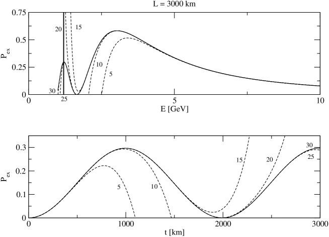
Figure 1: The neutrino oscillation probability $P_{ex}$ as a function of energy and time, respectively. Upper panel: The convergence of the energy spectrum given by our series expansion for a constant electron number density profile with $N_{e}=N_{e,\rm core}/3$. Lower panel: The convergence of the series expansion for $E=1.2$ GeV, corresponding to the bold line in the energy spectrum. The solid curves correspond to the exact solutions and the dashed curves correspond to the series expansion. The numbers correspond to the number of terms used in the series expansion. The solid vertical line in the upper panel corresponds to the energy used for the lower panel.

In this figure, we can observe that approximately 20 terms are needed to reconstruct one period of oscillation and that the convergence is indeed the same as for a simple trigonometric function.

IV.3 Linearly varying matter density

Now, we turn our interest towards the case of a linearly varying effective potential. In particular, we study a baseline of $L=3000$ km, where the electron number density is given by $N_{e}(t)=N_{e,\rm core}(t/L+1)/4$. As in the case of constant effective potential, it is again easy to obtain the coefficients $V_{n}$ from our equation for $V(t)$. Performing the numerical calculations result in Fig. 2.

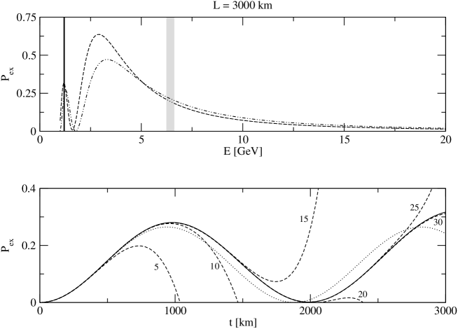
Figure 2: The energy spectrum of the neutrino oscillation probability $P_{ex}$ for a linear profile (upper panel) with $N_{e}=N_{e,\rm core}(1+t/L)/4$ along with the convergence of the solution for $E=1.2$ GeV (lower panel). In the energy spectra, the dotted curve corresponds to the numerical solution for the given profile, the dashed curve corresponds to our series solution, where we have included the first 35 terms, and the dash-dotted curve corresponds to an approximation of constant matter density. The solid vertical line corresponds to the energy used in the lower panel and the series solution is not plotted in the shaded region where it breaks down numerically. In the time evolution plot, the solid curve corresponds to the numerical solution, the dotted curve corresponds to the approximation of constant matter density, the dashed curves correspond to our series solution for different numbers of included terms, and the numbers correspond to the number of terms used for each of these curves.

In this figure, we have excluded the plot for our solution in the shaded region, which roughly corresponds to an energy equal to the resonance energy of the effective potential $V=V_{0}$, where the solution breaks down numerically. The reason for this breakdown can be found in Eq. (21), where we repeatedly divide by $F_{0}$. For the resonance energy corresponding to $V=V_{0}$, we have $F_{0}\sim 0$, which leads to large absolute values of numbers that should add up to a number between zero and one. Due to finite machine precision, we have numerical errors as a result.

Apart from neutrino energies near the resonance energy, we can observe that we again obtain a nice convergence of both the energy spectrum and the time evolution, where we reproduce one full oscillation by approximately 20 terms of our series expansion. It should be pointed out that this case of linearly varying matter density has no known application to experiments and only serves as an illustrative example.

IV.4 PREM profile

For the PREM electron number density profile, which is the interesting profile in, for example, long-baseline neutrino oscillation experiments, we use the expansion in Legendre polynomials and truncate the series using $N=2$ for definiteness. In effect, this corresponds to projecting the function $V(t)$, which is an element in the vector space of real functions on the interval $[0,L]$, onto the subspace of second order polynomial functions on $[0,L]$, using the inner product

$$\left<f,g\right>=\int_{0}^{L}f(x)g(x){\rm d}x.$$ (25)

In Fig. 3, we plot the electron number density profiles for the baseline lengths $L=250$ km, 750 km, 3000 km, and $5000$ km along with the second order polynomial approximations and the constant approximations.

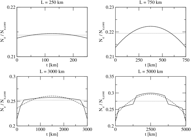
Figure 3: The matter density profiles for different baseline lengths $L$ according to the PREM. The solid curves are the exact profiles, the dashed curves are profiles approximated by a second order polynomial, and the dotted lines are the average matter densities, i.e., the matter density of approximations using constant electron number density. For $L=250$ km and 750 km the exact profiles and the approximations using a second order polynomial are practically the same and as a result they are not distinguishable in the figure.

In Fig. 4, we plot the energy spectra and time evolution at $E=1.2$ GeV for a baseline of $L=3000$ km for the PREM profile.

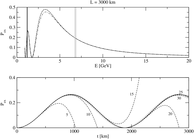
Figure 4: The energy spectrum for the neutrino oscillation probability $P_{ex}$ using 35 terms of our series solution (upper panel) and the convergence of the time evolution for $E=1.2$ GeV (lower panel). Here we assume a baseline of $L=3000$ km and using the PREM profile for the electron number density. In the energy spectrum, the dashed curve corresponds to the numerical solution using the PREM profile, the dotted curve corresponds to our series solution, and the dash-dotted curve corresponds to the approximation using constant matter density. The solid vertical line corresponds to the energy used in the lower panel and the series solution is not plotted in the shaded region where it breaks down numerically. In the time evolution plot, the solid curve corresponds to the numerical solution, the dotted curve to the solution for the constant matter density approximation, the dashed curves correspond to our series solution using different numbers of terms, and the numbers correspond to the number of terms used for each of these curves.

Again, our solution is not plotted in the shaded region in which it breaks down numerically for the same reasons as discussed previously. In this case, it is apparent that if the number of terms used in the series expansion is large enough, our solution is a significant improvement from the constant matter density approximation.

Clearly, the approximation of using a second order polynomial for the electron number density gives a very good reproduction of the numerical solution (which uses the profiles obtained from the PREM). As can be seen in the time evolution plot, the error made is barely noticeable until approximately one and a half oscillations, i.e., for lower neutrino energies if the baseline length $L$ is kept fixed. This is in good agreement with the results obtained in Ref. Ota and Sato (2001), where the effective potential is expanded in a Fourier series, as well as Ref. Ohlsson and Winter (2001), which shows that details of the effective potential that are smaller than the oscillation length cannot be resolved by neutrino oscillations. As noticed in both of the earlier cases, about 20 terms are needed in the series expansion in order to reproduce one full oscillation.

For the PREM profile, we are also interested in a number of other baseline lengths. In particular, in Fig. 5, we plot the energy spectra for the baseline lengths $L=250$ km, 750 km, 3000 km, and $5000$ km.

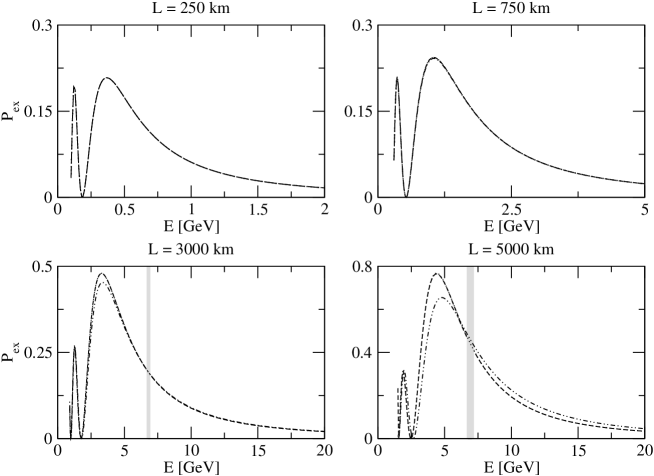
Figure 5: The energy spectra of the neutrino oscillation probability $P_{ex}$ for different baselines using the PREM profile for the electron number density. Again, we have used 35 terms from our series solution for each of these energy spectra and the dashed curves correspond to the numerical solutions, the dotted curves correspond to our series solution, and the dash-dotted curves correspond to the constant density approximations. The series solution is not plotted in the shaded regions where it breaks down numerically.

For the baseline lengths $L=250$ km and 750 km, there is no noticeable difference between the numerical solution, our exact solution, and the approximation using constant electron number density. This is to be expected as the electron number density does not vary significantly for these baseline lengths (see Fig. 3). However, for both $L=3000$ km and 5000 km, we do observe a difference between the constant electron number density approximations and the other two solutions. Again, we can conclude that the approximation with a second order polynomial for the electron number density agrees remarkably well with the numerical calculation using the profile obtained directly from the PREM. Note that the comparison of the energy spectra for different matter density profiles and baselines has been studied before Freund and Ohlsson (2000).

For baselines longer than $L=5000$ km, the region near the resonance for $V=V_{0}$ tends to expand and ruin the numerical convergence of our solution. Also, this region expands if we include more terms of the series expansion. For the baseline lengths below $L=5000$ km, this can be somewhat compensated by using fewer terms of the series expansion for high energies to avoid the numerical cancellation effects and more terms for lower energies to obtain a nice convergence.

V Other methods of solving the neutrino flavor evolution

In general, there have been numerous methods on how to solve the problem of neutrino flavor evolution in matter Wolfenstein (1978); Ohlsson and Snellman (2000a); Akhmedov (1988); Barger et al. (1980); Lehmann et al. (2001); Osland and Wu (2000); Smirnov (1987); Balantekin et al. (1988); Ioannisian and Smirnov (2004); Fishbane and Gasiorowicz (2001). First of all, there is the obvious formal solution using a time-ordered exponential, i.e.,

$$\left|\nu(t)\right\rangle=T\left[\exp\left(-{\rm i}\int_{0}^{t}H(\tau){\rm d}\tau\right)\right]\left|\nu(0)\right\rangle.$$ (26)

This solution is exact, but it is not very helpful in actual calculations due to the nature of the time-ordered exponential. A way of solving this problem is to use a discretization of the effective potential Ohlsson and Snellman (2000a). The effective potential is then divided into a finite number of layers with constant effective potentials (i.e., constant electron number density), which approximate a given effective potential. Clearly, when the number of layers goes to infinity, one regains the time-ordered exponential.

There is also the pure numerical approach to the problem, where the neutrino flavor evolution is easily solved numerically for any effective potential. While this gives the possibility of actually calculating numerical values for the neutrino oscillation probabilities, it does not offer any insight into how these probabilities vary with different parameters.

In addition, the neutrino flavor evolution can be analytically solved for some specific effective potentials. Examples are the constant (two flavors Wolfenstein (1978) and three flavors Barger et al. (1980)), linearly Lehmann et al. (2001) and exponentially Osland and Wu (2000) varying effective potentials.

Moreover, a widely used solution is the adiabatic solution Smirnov (1987); Balantekin et al. (1988), where the effective potential is assumed to change slowly, so that there are no transitions between different matter eigenstates of the full Hamiltonian. This approximation can be derived by, for example, using the Wentzel–Kramers–Brillouin (WKB) method Balantekin et al. (1988), where also higher order corrections due to non-adiabatic transitions can be calculated.

There have also been earlier efforts to write the neutrino evolution equations as ordinary non-linear differential equations, see for example Ref. Fishbane and Gasiorowicz (2001). However, such equations have generally been complex differential equations for the probability amplitudes and not, as in the present case, real differential equations for the probabilities. Also, the solutions in such cases have been made for special cases of the effective potential and not as series solutions valid for all effective potentials.

Lately, approximate solutions, valid when the effective potential $V\ll\Delta m^{2}/(2E)$, have been presented Ioannisian and Smirnov (2004) and applied to oscillations of solar neutrinos and the solar neutrino day-night effect. However, these solutions are not valid for the baseline lengths and neutrino energies which we have treated numerically.

VI Summary and conclusions

We have shown that solving the general problem of two flavor neutrino oscillations with an arbitrary effective potential is equivalent with solving the non-linear ordinary differential equation

$$(\ddot{p}+Gp)^{2}=F(t)[G(1-p^{2})-\dot{p}^{2}],$$ (27)

where $G\equiv[\Delta m^{2}/(2E)]^{2}\sin^{2}(2\theta)$, $F(t)\equiv[\Delta m^{2}\cos(2\theta)/(2E)-V(t)]^{2}$, and the neutrino oscillation probability $P_{ex}$ is given by

$$P_{ex}=\frac{1}{2}(1-p).$$ (28)

We have presented an exact solution [see Eqs. (21) and (22)] to this equation by adopting the method of series expansion of both the solution and the effective potential $V(t)$ and demonstrated the numerical convergence of this solution for a number of different effective potentials. In all cases investigated, about 20 terms in the series expansion are required to reproduce one period of oscillation. We have also seen that for the neutrino energies and baselines considered, the energy spectra of the neutrino oscillation probability is well reproduced by approximating the effective potential by a second order polynomial.

- (1) C. W. Kim and A. Pevsner, Neutrinos in Physics and Astrophysics, Chur, Switzerland: Harwood (1993) 429 p. (Contemporary concepts in physics, 8).
- Cleveland et al. (1998) B. T. Cleveland et al., Astrophys. J. 496, 505 (1998); J. N. Abdurashitov et al. (SAGE Collaboration), J. Exp. Theor. Phys. 95, 181 (2002), eprint astro-ph/0204245; W. Hampel et al. (GALLEX Collaboration), Phys. Lett. B447, 127 (1999); M. Altmann et al. (GNO Collaboration), Phys. Lett. B490, 16 (2000), eprint hep-ex/0006034; S. Fukuda et al. (Super-Kamiokande Collaboration), Phys. Lett. B539, 179 (2002), eprint hep-ex/0205075; Q. R. Ahmad et al. (SNO Collaboration), Phys. Rev. Lett. 89, 011301 (2002), eprint nucl-ex/0204008; S. N. Ahmed et al. (SNO Collaboration), eprint nucl-ex/0309004.
- Fukuda et al. (1998) Y. Fukuda et al. (Super-Kamiokande Collaboration), Phys. Rev. Lett. 81, 1562 (1998), eprint hep-ex/9807003; 82, 2644 (1999), eprint hep-ex/9812014; M. Ambrosio et al. (MACRO Collaboration), Phys. Lett. B566, 35 (2003), eprint hep-ex/0304037.
- Apollonio et al. (1999) M. Apollonio et al. (CHOOZ Collaboration), Phys. Lett. B466, 415 (1999), eprint hep-ex/9907037.
- Apollonio et al. (2003) M. Apollonio et al. (CHOOZ Collaboration), Eur. Phys. J. C27, 331 (2003), eprint hep-ex/0301017.
- Ahn et al. (2003) M. H. Ahn et al. (K2K Collaboration), Phys. Rev. Lett. 90, 041801 (2003), eprint hep-ex/0212007; K. Eguchi et al. (KamLAND Collaboration), Phys. Rev. Lett. 90, 021802 (2003), eprint hep-ex/0212021.
- Wolfenstein (1978) L. Wolfenstein, Phys. Rev. D17, 2369 (1978).
- Mikheyev and Smirnov (1985) S. P. Mikheyev and A. Y. Smirnov, Sov. J. Nucl. Phys. 42, 913 (1985), Yad. Fiz. 42, 1441 (1985); Nuovo Cim. C9, 17 (1986).
- Ohlsson and Snellman (2000a) T. Ohlsson and H. Snellman, Phys. Lett. B474, 153 (2000a), B480, 419(E) (2000), eprint hep-ph/9912295.
- Akhmedov (1988) E. K. Akhmedov, Sov. J. Nucl. Phys. 47, 301 (1988), Yad. Fiz. 47, 475 (1988); Nucl. Phys. B538, 25 (1999a), eprint hep-ph/9805272; S. T. Petcov, Phys. Lett. B434, 321 (1998), eprint hep-ph/9805262.
- Barger et al. (1980) V. D. Barger, K. Whisnant, S. Pakvasa, and R. J. N. Phillips, Phys. Rev. D22, 2718 (1980); C. W. Kim and W. K. Sze, Phys. Rev. D35, 1404 (1987); H. W. Zaglauer and K. H. Schwarzer, Z. Phys. C40, 273 (1988); T. Ohlsson and H. Snellman, J. Math. Phys. 41, 2768 (2000b), 42, 2345(E) (2001), eprint hep-ph/9910546.
- Lehmann et al. (2001) H. Lehmann, P. Osland, and T. T. Wu, Commun. Math. Phys. 219, 77 (2001), eprint hep-ph/0006213.
- Osland and Wu (2000) P. Osland and T. T. Wu, Phys. Rev. D62, 013008 (2000), eprint hep-ph/9912540.
- Smirnov (1987) A. Y. Smirnov, Sov. J. Nucl. Phys. 46, 672 (1987), Yad. Fiz. 46, 1152 (1987); T. K. Kuo and J. Pantaleone, Phys. Rev. D35, 3432 (1987); S. Toshev, Phys. Lett. B185, 177 (1987); S. T. Petcov, Phys. Lett. B191, 299 (1987); B214, 259 (1988); S. T. Petcov and S. Toshev, Phys. Lett. B187, 120 (1987); P. Langacker, S. T. Petcov, G. Steigman, and S. Toshev, Nucl. Phys. B282, 589 (1987).
- Balantekin et al. (1988) A. B. Balantekin, S. H. Fricke, and P. J. Hatchell, Phys. Rev. D38, 935 (1988); A. Nicolaidis, Phys. Lett. B242, 480 (1990).
- Ioannisian and Smirnov (2004) P. C. de Holanda, W. Liao and A. Y. Smirnov, eprint hep-ph/0404042; A. N. Ioannisian and A. Y. Smirnov, eprint hep-ph/0404060; E. K. Akhmedov, M. A. Tórtola, and J. W. F. Valle, eprint hep-ph/0404083.
- Fishbane and Gasiorowicz (2001) P. M. Fishbane and S. G. Gasiorowicz, Phys. Rev. D64, 113017 (2001), eprint hep-ph/0012230.
- Dziewonski and Anderson (1981) A. M. Dziewonski and D. L. Anderson, Phys. Earth Planet. Interiors 25, 297 (1981).
- (19) Y. Hayato (Super-Kamiokande Collaboration), talk at the HEP2003 conference (Aachen, Germany, 2003), http://eps2003.physik.rwth-aachen.de.
- Bilenky and Petcov (1987) S. M. Bilenky and S. T. Petcov, Rev. Mod. Phys. 59, 671 (1987); E. K. Akhmedov, eprint hep-ph/0001264.
- Ota and Sato (2001) T. Ota and J. Sato, Phys. Rev. D63, 093004 (2001), eprint hep-ph/0011234.
- Ohlsson and Winter (2001) T. Ohlsson and W. Winter, Phys. Lett. B512, 357 (2001), eprint hep-ph/0105293.
- Freund and Ohlsson (2000) M. Freund and T. Ohlsson, Mod. Phys. Lett. A15, 867 (2000), eprint hep-ph/9909501, and references therein.