Spectra and decays of $\pi\pi$
and $\pi K$ atoms

J. Schweizer

Institute for Theoretical Physics,

University of Bern,

Sidlerstr. 5, CH–3012 Bern, Switzerland

E-mail: schweizer@itp.unibe.ch

May 5, 2004

We describe the spectra and decays of $\pi^{+}\pi^{-}$ and $\pi^{\pm}K^{\mp}$ atoms within a non-relativistic effective field theory. The evaluations of the energy shifts and widths are performed at next-to-leading order in isospin symmetry breaking. We provide general formulae for all S-states, and discuss the states with angular momentum one in some detail. The prediction for the lifetime of the $\pi^{\pm}K^{\mp}$ atom in its ground-state yields $\tau_{10}=(3.7\pm 0.4)\cdot 10^{-15}$s.

Pacs number(s):	03.65.Ge, 03.65.Nk, 11.10.St, 12.39.Fe, 13.40.Ks
Keywords:	Hadronic atoms, Chiral perturbation theory, Pion-pion scattering
	lengths, Pion-kaon scattering lengths, Non relativistic effective
	Lagrangians, Isospin symmetry breaking, Electromagnetic corrections

1 Introduction

The DIRAC collaboration [1] at CERN has measured the lifetime of pionium in its ground-state, and the preliminary result yields $\tau_{\pi,10}=[3.1^{+0.9}_{-0.7}({\rm stat})\pm 1({\rm syst})]\cdot 10^{-15}$s [2]. A lifetime measurement of pionium at the $10\%$ level allows one to determine the S-wave $\pi\pi$ scattering length difference $|a_{0}^{0}-a_{0}^{2}|$ at $5\%$ accuracy. The measurement can then be compared with theoretical predictions for the S-wave scattering lengths [3, 4, 5] and with the results coming from scattering experiments [6]. Particularly exciting is the fact that this enterprise subjects chiral perturbation theory to a very sensitive test [7]. New measurements are proposed for CERN PS, J-PARC and GSI [8]. These experiments aim to measure the lifetime of $\pi^{+}\pi^{-}$ and $\pi^{\pm}K^{\mp}$ atoms simultaneously.

In order to extract the scattering lengths from such future precision measurements, the theoretical expressions for the energy shifts and decay widths of the $\pi^{+}\pi^{-}$ and $\pi^{\pm}K^{\mp}$ atoms must be known to a precision that matches the experimental accuracy. Nearly fifty years ago, Deser et al. [9] derived the leading order formulae for the decay width and the energy shift in pionic hydrogen. Similar relations exist for $\pi^{+}\pi^{-}$ and $\pi^{\pm}K^{\mp}$ atoms [10, 11], which decay due to the strong interactions into $2\pi^{0}$ and $\pi^{0}K^{0}$, respectively. Theoretical investigations on the spectrum and the decay of pionium have been performed beyond leading order in several settings. Potential scattering has been used [12, 13, 14] as well as field-theoretical methods [15, 16, 17, 18, 19, 20]. In particular, the lifetime of pionium was studied by the use of the Bethe-Salpeter equation [19] and in the framework of the quasipotential-constraint theory approach [20]. The width of the $\pi^{+}\pi^{-}$ atom has also been analyzed within a non-relativistic effective field theory [21, 22, 23], which was originally developed for bound states in QED by Caswell and Lepage [24]. The non-relativistic framework has proven to be a very efficient method to evaluate bound state characteristics. It was further applied to the ground-state of pionic hydrogen [25, 26, 27] and very recently to the energy-levels and decay widths of kaonic hydrogen [28]. Within the non-relativistic effective field theory the isospin symmetry breaking corrections to the Deser-type formulae can be evaluated systematically. In Refs. [21, 22, 23, 29, 30] the lifetime of pionium was evaluated at next-to-leading order in the isospin breaking parameters $\alpha\simeq 1/137$ and $(m_{u}-m_{d})^{2}$.

We presented in Ref. [31], the results for the S-wave decay widths and strong energy shifts of $\pi^{+}\pi^{-}$ and $\pi^{\pm}K^{\mp}$ atoms at next-to-leading order in isospin symmetry breaking. Further, for the lifetime as well as for the first two energy-level shifts, a numerical analysis was carried out. The aim of this article is to provide the details that have been omitted in Ref. [31]. Chiral perturbation theory (ChPT) allows one to relate the result for the width of the $\pi^{\pm}K^{\mp}$ atom to the isospin odd $\pi K$ scattering lengths $a_{0}^{-}$, while the strong energy shift is proportional to the sum of isospin even and odd scattering lengths $a_{0}^{+}+a_{0}^{-}$. The values for $a_{0}^{+}$ and $a_{0}^{-}$, used in the numerical evaluation of the widths and strong energy shifts, stem from the recent analysis of $\pi K$ scattering from Roy and Steiner type equations [33]. Within ChPT, the $\pi K$ scattering lengths have been worked out at one–loop accuracy [34, 35, 36], and very recently even the chiral expansion of the $\pi K$ scattering amplitude at next-to-next-to-leading order became available [37]. Particularly interesting is that the isospin even scattering lengths $a_{0}^{+}$ depends on the low–energy constant $L_{6}^{r}$ [38], and this coupling is related to the flavour dependence of the quark condensate [39].

The paper is organized as follows: The general features of $\pi^{+}\pi^{-}$ and $\pi^{\pm}K^{\mp}$ atoms are described in Section 2. The non-relativistic effective field-theory approach is illustrated in Section 3 by means of the $\pi^{-}K^{+}$ atom. The discussion includes the Hamiltonian, the master equation, and the matching to the relativistic $\pi K$ amplitudes. In Sec. 4, we present the results for the decay widths and strong energy shifts of the $\pi^{\pm}K^{\mp}$ and $\pi^{+}\pi^{-}$ atoms at next-to-leading order in isospin symmetry breaking. The role of transverse photons is discussed in Section 5. Transverse photons do contribute to the electromagnetic part of the energy shift. The pure QED contributions have been worked out a long time ago, based on the Bethe-Salpeter equation [40], the quasipotential approach [41, 42] and an improved Coulomb potential [43]. We reproduced this result within the non-relativistic framework. We further estimate the contributions from transverse photons to the decay width of the $\pi^{-}K^{+}$ atom and show that they vanish at next-to-leading order in isospin symmetry breaking. The contributions generated by the vacuum polarization of the electron [22, 25, 44] are discussed in Section 6. Formally of higher order in $\alpha$, they are numerically not negligible. A numerical analysis of the widths and the energy-level shifts is carried out in Section 7 at $\mathcal{O}(p^{4},e^{2}p^{2})$ in the chiral expansion.

2 General features of $\pi\pi$ and $\pi K$ atoms

In this section, we describe the general features of the systems that we are going to study. The $\pi^{+}\pi^{-}$ and $\pi^{\pm}K^{\mp}$ atoms are highly non-relativistic, loosely bound systems, mainly formed by the Coulomb interaction. The average momentum of the constituents in the c.m. frame lies in the MeV range. Further, their decay widths $\sim 0.2$eV are much smaller than the binding energies $\sim 10^{3}$eV involved. The $\pi^{+}\pi^{-}$ atom in its ground-state decays predominantly into a pair of two neutral pions, through the strong transition $\pi^{+}\pi^{-}\rightarrow\pi^{0}\pi^{0}$. The decay width into two photons is suppressed by the factor $4\cdot 10^{-3}$ [1, 29]. For a detailed discussion of the decay channels of pionium, we refer to [23]. The decays of the $\pi^{-}K^{+}$ atom have to conserve strangeness. Apart from the dominant S-wave decay channel into $\pi^{0}K^{0}$, the only allowed decays are therefore $K^{0}+n_{1}\gamma+n_{2}e^{+}e^{-}$ and $\pi^{0}K^{0}+n_{1}\gamma+n_{2}e^{+}e^{-}$, where $n_{1}+n_{2}>0$. Here $n_{1}$ and $n_{2}$ denotes the number of photons and $e^{+}e^{-}$ pairs, respectively. In the relativistic theory, the odd intrinsic parity process $\pi^{-}K^{+}\rightarrow K^{0}+2\gamma$ corresponds to a local interaction in the Wess-Zumino-Witten term [45], while the transition $\pi^{-}K^{+}\rightarrow K^{0}+\gamma$ occurs not until $\mathcal{O}(p^{6})$ [46].

The non-relativistic framework [21, 23, 24, 25] we are going to apply, provides a systematic expansion in the isospin breaking parameter $\delta$. In the case of pionium, we count $\alpha$ as well as $(m_{u}-m_{d})^{2}$ as small quantities of order $\delta$. As for the $\pi^{\pm}K^{\mp}$ atom, both $\alpha$ and $m_{u}-m_{d}$ count as order $\delta$. The different power counting schemes are due to the fact that in QCD, the chiral expansion of the pion mass squared difference $\Delta_{\pi}=M_{\pi^{\scriptscriptstyle{+}}}^{2}-M_{\pi^{\scriptscriptstyle{0}}}^{2}$ is of second order in $m_{u}-m_{d}$, while $\Delta_{K}=M_{\scriptscriptstyle{K^{+}}}^{2}-M_{\scriptscriptstyle{K^{0}}}^{2}$ is linear in $m_{u}-m_{d}$. At leading and next-to-leading order in isospin symmetry breaking, the $\pi^{+}\pi^{-}$, ($\pi^{-}K^{+}$) atom decays into $\pi^{0}\pi^{0}$ ($\pi^{0}K^{0}$) exclusively. The leading order term for the width is of $\mathcal{O}(\delta^{7/2})$, isospin breaking corrections contribute at order $\delta^{9/2}$. The results for the S-wave decay widths at order $\delta^{9/2}$ are presented in Secs. 4.1 and 4.3. At order $\delta^{5}$, also other decay channels contribute. In Section 5.2, we estimate the order of the various decays.

The energy-level splittings of the $\pi^{+}\pi^{-}$ and $\pi^{\pm}K^{\mp}$ atoms are induced by both electromagnetic and strong interactions. At order $\delta^{3}$, the energy shift contributions are exclusively due to strong interactions, while at order $\delta^{4}$, both electromagnetic and strong interactions contribute. It is both conventional and convenient to split the energy shifts into a strong and an electromagnetic part, according to

$$\Delta E_{nl}=\Delta E^{\rm h}_{nl}+\Delta E^{\rm em}_{nl}.$$ (2.1)

The expressions for the strong energy shift $\Delta E^{\rm h}_{nl}$ at next-to-leading order in isospin symmetry breaking are presented in Secs. 4.2 and 4.3. The electromagnetic part $\Delta E^{\rm em}_{nl}$ is discussed in Section 5.1. Another important correction is generated by the vacuum polarization of the electron. Formally, the vacuum polarization contributes to the energy shift at order $\delta^{5}$ and to the width at order $\delta^{11/2}$, but these corrections are amplified by powers of the ratio $\mu_{+}/m_{e}$. Here $\mu_{+}$ denotes the reduced mass of the bound system and $m_{e}$ the electron mass. The vacuum polarization contributions are discussed in Section 6.

In what follows, we proceed systematically and discuss in detail the decays and bound state spectra within the non-relativistic framework.

3 Non-relativistic framework

3.1 Hamiltonian

The Hamiltonian consists of a infinite series of operators with increasing mass dimensions - all operators allowed by gauge invariance, space rotation, parity and time reversal must be included. However, in the evaluation of the decay width and the strong energy shift at next-to-leading order in isospin symmetry breaking, only a few low dimensional operators do actually contribute. For the $\pi^{-}K^{+}$ atom, the following Hamiltonian achieves the goal:

$${\bf{H}} = {\bf{H}}_{0}+{\bf{H}}_{\scriptscriptstyle\rm C}+{\bf{H}}_{\scriptscriptstyle\rm D}+{\bf{H}}_{\scriptscriptstyle\rm S},$$

$${\bf{H}}_{\rm\Gamma} = \int d^{3}{\bf{x}}\,\mathcal{H}_{\rm\Gamma}(0,{\bf{x}}),\quad{\rm\Gamma}={\rm 0,C,D,S},$$ (3.1)

with

$$\mathcal{H}_{0} = \sum_{i=\pm,0}\left\{\pi_{i}^{\dagger}\left(M_{\pi^{i}}-\frac{\Delta}{2M_{\pi^{i}}}\right)\pi_{i}+K_{i}^{\dagger}\left(M_{\scriptscriptstyle K^{i}}-\frac{\Delta}{2M_{\scriptscriptstyle K^{i}}}\right)K_{i}\right\},$$

$$\mathcal{H}_{\scriptscriptstyle\rm D} = -\sum_{i=\pm,0}\left\{\pi_{i}^{\dagger}\left(\frac{\Delta^{2}}{8M_{\pi^{i}}^{3}}+\cdots\right)\pi_{i}+K_{i}^{\dagger}\left(\frac{\Delta^{2}}{8M_{\scriptscriptstyle K^{i}}^{3}}+\cdots\right)K_{i}\right\},$$

$$\mathcal{H}_{\scriptscriptstyle\rm C} = -2\pi\alpha\left(\sum_{\pm}\pm\pi_{\pm}^{\dagger}\pi_{\pm}\pm K_{\pm}^{\dagger}K_{\pm}\right)\Delta^{-1}\left(\sum_{\pm}\pm\pi_{\pm}^{\dagger}\pi_{\pm}\pm K_{\pm}^{\dagger}K_{\pm}\right),$$

$$\mathcal{H}_{\scriptscriptstyle\rm S} = -C_{1}\pi_{\scriptscriptstyle{-}}^{\dagger}K_{\scriptscriptstyle{+}}^{\dagger}\pi_{\scriptscriptstyle{-}}K_{\scriptscriptstyle{+}}-C_{2}\left(\pi_{\scriptscriptstyle{-}}^{\dagger}K_{\scriptscriptstyle{+}}^{\dagger}\pi_{\scriptscriptstyle{0}}K_{\scriptscriptstyle{0}}+\textrm{h.c}\right)-C_{3}\pi_{\scriptscriptstyle{0}}^{\dagger}K_{\scriptscriptstyle{0}}^{\dagger}\pi_{\scriptscriptstyle{0}}K_{\scriptscriptstyle{0}}$$ (3.2)

$$-C_{4}\left(\pi_{\scriptscriptstyle{-}}^{\dagger}{\scriptscriptstyle\overleftrightarrow{\textstyle\Delta}}K_{\scriptscriptstyle{+}}^{\dagger}\pi_{\scriptscriptstyle{0}}K_{\scriptscriptstyle{0}}+\textrm{h.c}\right)-C_{5}\left(\pi_{\scriptscriptstyle{-}}^{\dagger}{\scriptscriptstyle\overleftrightarrow{\textstyle\Delta}}K_{\scriptscriptstyle{+}}^{\dagger}\pi_{\scriptscriptstyle{-}}K_{\scriptscriptstyle{+}}+{\rm h.c}\right)$$

$$-C_{6}(\pi_{\scriptscriptstyle{-}}^{\dagger}\pi_{\scriptscriptstyle{-}})\Delta(K_{\scriptscriptstyle{+}}^{\dagger}K_{\scriptscriptstyle{+}})-C_{7}\left(\nabla\pi_{\scriptscriptstyle{-}}^{\dagger}K_{\scriptscriptstyle{+}}^{\dagger}\nabla\pi_{\scriptscriptstyle{0}}K_{\scriptscriptstyle{0}}+\textrm{h.c}\right)+\cdots,$$

where $u{\scriptscriptstyle\overleftrightarrow{\textstyle\Delta}}v\doteq u\Delta v+v\Delta u$. We work in the c.m. system and thus omit terms proportional to the c.m. momentum. The basis of operators with two space derivatives is chosen such that none of them contributes to the S-wave decay width and energy shift at the accuracy we are considering. For this reason, we transformed the operator with two space derivatives on the neutral fields by the use of the equations of motion,

$$\pi_{\scriptscriptstyle{-}}^{\dagger}K_{\scriptscriptstyle{+}}^{\dagger}\pi_{\scriptscriptstyle{0}}{\scriptscriptstyle\overleftrightarrow{\textstyle\Delta}}K_{\scriptscriptstyle{0}}=-4\mu_{0}(\Sigma_{+}-\Sigma_{0})\pi_{\scriptscriptstyle{-}}^{\dagger}K_{\scriptscriptstyle{+}}^{\dagger}\pi_{\scriptscriptstyle{0}}K_{\scriptscriptstyle{0}}+\frac{\mu_{0}}{\mu_{+}}\pi_{\scriptscriptstyle{-}}^{\dagger}{\scriptscriptstyle\overleftrightarrow{\textstyle\Delta}}K_{\scriptscriptstyle{+}}^{\dagger}\pi_{\scriptscriptstyle{0}}K_{\scriptscriptstyle{0}}.$$ (3.3)

For the moment, we further neglect transverse photon contributions. To the accuracy we are working, they do not contribute to the decay width and to the strong energy-level shifts. However, transverse photons do contribute when we work out the electromagnetic energy-level shifts in Section 5.1. The non-relativistic Lagrangian in the presence of transverse photons is given in appendix A. The Hamiltonian in Eq. (3.1) is built from the non-relativistic pion and kaon fields

$$\pi_{i}(0,{\bf{x}})=\int d\nu({\bf{p}})e^{i{\bf{p}}{\bf{x}}}{\bf{a}}_{i}({\bf{p}}),\quad K_{i}(0,{\bf{x}})=\int d\nu({\bf{p}})e^{i{\bf{p}}{\bf{x}}}{\bf{b}}_{i}({\bf{p}}),\quad i=\pm,0,$$ (3.4)

with $d\nu({\bf{p}})\doteq d^{3}{\bf{p}}/(2\pi)^{3}$ and

$$\left[{\bf{a}}_{i}({\bf{p}}),{\bf{a}}_{k}^{\dagger}({\bf{p}}^{\prime})\right] = (2\pi)^{3}\delta^{3}({\bf{p}}-{\bf{p}}^{\prime})\delta_{ik},$$

$$\left[{\bf{b}}_{i}({\bf{p}}),{\bf{b}}_{k}^{\dagger}({\bf{p}}^{\prime})\right] = (2\pi)^{3}\delta^{3}({\bf{p}}-{\bf{p}}^{\prime})\delta_{ik}.$$ (3.5)

The two particle states of zero total charge are defined by

$$\mid\!{\bf{p}}_{1},{\bf{p}}_{2}\rangle_{+}={\bf{a}}_{-}^{\dagger}({\bf{p}}_{1}){\bf{b}}_{+}^{\dagger}({\bf{p}}_{2})\mid\!0\rangle,\quad\mid\!{\bf{p}}_{3},{\bf{p}}_{4}\rangle_{0}={\bf{a}}_{0}^{\dagger}({\bf{p}}_{3}){\bf{b}}_{0}^{\dagger}({\bf{p}}_{4})\mid\!0\rangle,$$ (3.6)

and the total and reduced masses $\Sigma_{i}$ and $\mu_{i}$ respectively, read

$$\Sigma_{i}=M_{\pi^{i}}+M_{\scriptscriptstyle K^{i}},\quad\mu_{i}=\frac{M_{\pi^{i}}M_{\scriptscriptstyle K^{i}}}{M_{\pi^{i}}+M_{\scriptscriptstyle K^{i}}},\quad i=+,0.$$ (3.7)

3.2 Master equation

To evaluate the decay width and the strong energy shifts we make use of resolvents. This technique, which was developed by Feshbach a long time ago [47], has been discussed extensively in Ref. [23]. To remove the center of mass momentum from the matrix elements of any operators ${\bf{R}}$, we introduce the notation

$${}_{a}\langle{\bf{p}}_{1},{\bf{p}}_{2}\!\mid\mbox{\boldmath$\bf R$}(z)\mid\!{\bf{p}}_{3},{\bf{p}}_{4}\rangle_{b}$$ (3.8)

$$= (2\pi)^{3}\delta^{3}({\bf{p}}_{1}+{\bf{p}}_{2}-{\bf{p}}_{3}-{\bf{p}}_{4}){}_{a}({\bf{p}}_{1},{\bf{p}}_{2}\!\mid\mbox{\boldmath$\bf R$}(z)\mid\!{\bf{p}}_{3},{\bf{p}}_{4})_{b},$$

where $a,b$ stand for $0,+$. Further, we have

$${}_{a}\!({\bf{q}},-{\bf{q}}\!\mid{\bf{R}}(z)\mid\!{\bf{p}},-{\bf{p}})_{b}\doteq{}_{a}\!({\bf{q}}\!\mid{\bf{R}}(z)\mid\!{\bf{p}})_{b}.$$ (3.9)

The master formula to be solved is given by the following eigenvalue equation,

$$z-E_{n}-\int d\nu({\bf{P}})\langle\Psi_{n0},{\bf{P}}\!\mid\mbox{\boldmath$\bf\bar{\tau}$}(z)\mid\!\Psi_{n0},0\rangle=0,$$ (3.10)

where $E_{n}=\Sigma_{+}-\alpha^{2}\mu_{+}/(2n^{2})$ denotes the $n$-th Coulomb energy and the unperturbed $n$-th eigenstate is given by

$$\mid\!\Psi_{n0},{\bf{P}}\rangle=\int d\nu({\bf{q}})\Psi_{n0}({\bf{q}})\mid\!\tfrac{\mu_{+}}{M_{\scriptscriptstyle{K^{+}}}}{\bf{P}}+{\bf{q}},\tfrac{\mu_{+}}{M_{\pi^{\scriptscriptstyle{+}}}}{\bf{P}}-{\bf{q}}\rangle_{+}.$$ (3.11)

Here $\Psi_{n0}({\bf{q}})$ stands for the Coulomb wave function of the bound $\pi^{\pm}K^{\mp}$ system in momentum space. The operator $\bf\bar{\tau}$, defined through

$$\mbox{\boldmath$\bf\bar{\tau}$}={\bf{V}}+{\bf{V}}{\bf{\bar{G}}}^{n}_{\scriptscriptstyle\rm C}\mbox{\boldmath$\bf\bar{\tau}$},\quad{\bf{V}}={\bf{H}}_{\scriptscriptstyle\rm D}+{\bf{H}}_{\scriptscriptstyle\rm S},$$ (3.12)

is regular in the vicinity of $E_{n}$. The quantity ${\bf{\bar{G}}}^{n}_{\scriptscriptstyle\rm C}$ stands for the $n$-th energy eigenstate singularity removed Coulomb resolvent,

$${\bf{\bar{G}}}^{n}_{\scriptscriptstyle\rm C}={\bf{G}}_{\scriptscriptstyle\rm C}\bigg{\{}{\bf{1}}-\int d\nu({\bf{P}})\mid\!\Psi_{n0},{\bf{P}}\rangle\langle\Psi_{n0},{\bf{P}}\!\mid\bigg{\}},\quad{\bf{G}}_{\scriptscriptstyle\rm C}=\frac{1}{z-{\bf{H}}_{0}-{\bf{H}}_{\scriptscriptstyle\rm C}}.$$ (3.13)

The master equation presents a compact form of the Rayleigh-Schrödinger perturbation theory. If we insert $\bf\bar{\tau}$ iteratively into (3.10), the eigenvalue equation becomes

$$z=E_{n}-|\Psi_{n0}({\bf{x}}=0)|^{2}\left[C_{1}+C_{2}^{2}J_{0}(z)\right]+\cdots$$ (3.14)

where $\Psi_{n0}({\bf{x}}=0)$ stands for the Coulomb wave function in coordinate space and $J_{0}$ denotes the loop integral in Eq. (D.3). The function $J_{0}$ is analytic in the complex $z$ plane, except for a cut on the real axis starting at $z=\Sigma_{0}$. The imaginary part of $J_{0}$ has the same sign as ${\rm\,Im}\,z$ throughout the cut $z$ plane, which does not allow Eq. (3.14) to have a solution on the first Riemann sheet. However, if we analytically continue $J_{0}$ from the upper rim of the cut to the second Riemann sheet, we find a solution at $z={\rm Re}\,z+i\,{\rm Im}\,z$, with

$${\rm Re\,}z=E_{n}-\frac{\alpha^{3}\mu_{+}^{3}C_{1}}{\pi n^{3}}+\cdots,\quad{\rm Im\,}z=-\frac{\alpha^{3}\mu_{+}^{3}\mu_{0}}{2\pi^{2}n^{3}}C_{2}^{2}\sqrt{\rho_{n}}+\cdots,$$ (3.15)

and $\rho_{n}=2\mu_{0}\left(E_{n}-\Sigma_{0}\right)$. In the following, we evaluate the S-wave decay width $\Gamma_{n0}=-2{\rm Im}\,z$ at order $\delta^{9/2}$ and the energy shift $\Delta E_{n0}={\rm Re}\,z-E_{n}$ at order $\delta^{4}$. We focus on the strong part of the energy shift only, the evaluation of the electromagnetic energy shift is discussed in Section 5.1. As in Ref. [23], we reduce Eq. (3.10) to a one-channel problem with an effective potential ${\bf{W}}$,

$$\varrho\mbox{\boldmath$\bf\bar{\tau}$}\varrho=\varrho{\bf{W}}\varrho+\varrho{\bf{W}}\varrho\mbox{\boldmath$\bf\bar{G}$}^{n}_{\scriptscriptstyle\rm C}\varrho\mbox{\boldmath$\bf\bar{\tau}$}\varrho,$$ (3.16)

where

$${\bf{W}}={\bf{V}}+{\bf{V}}\varrho_{0}\mbox{\boldmath$\bf\bar{G}$}_{\scriptscriptstyle\rm C}^{n}\left\{{\bf{1}}-\varrho_{0}{\bf{V}}\varrho_{0}\mbox{\boldmath$\bf\bar{G}$}_{\scriptscriptstyle\rm C}^{n}\right\}^{-1}\varrho_{0}{\bf{V}}.$$ (3.17)

Here $\varrho$, ($\varrho_{0}$) denotes the charged (neutral) two-particle projector

$$\varrho=\int d\nu({\bf{p}}_{1})d\nu({\bf{p}}_{2})\mid\!{\bf{p}}_{1},{\bf{p}}_{2}\rangle_{+}{}_{+}\!\langle{\bf{p}}_{1},{\bf{p}}_{2}\!\mid,\quad\varrho_{0}={\bf{1}}-\varrho.$$ (3.18)

The matrix element of ${\bf{W}}$ between charged states takes the form:

$${}_{+}\!({\bf{q}}\!\mid{\bf{W}}(z)\mid\!{\bf{p}})_{+} = (2\pi)^{3}\delta^{3}({\bf{q}}-{\bf{p}})\left[-\frac{{\bf{p}}^{4}}{8}\left(\frac{1}{M_{\pi^{\scriptscriptstyle{+}}}^{3}}+\frac{1}{M_{\scriptscriptstyle{K^{+}}}^{3}}\right)+\cdots\right]$$

$$+w(z)+w_{1}(z){\bf{p}}^{2}+w_{2}(z){\bf{q}}^{2}+w_{3}(z){\bf{p}}{\bf{q}}+\cdots$$

To the accuracy we are working, only the constant term $w(z)$ contributes to the decay width and strong energy shift. We get for the S-wave decay width of the $\pi^{-}K^{+}$ atom at order $\delta^{9/2}$,

$$\Gamma_{n0}=-2\mid\!\Psi_{n0}({\bf{x}}=0)\!\mid^{2}{\rm Im}\,w(E_{n})\left(1+2{\rm Re}\,w(E_{n})\langle{\bf{\bar{g}}}^{n}_{\scriptscriptstyle\rm C}(E_{n})\rangle\right)+\mathcal{O}(\delta^{5}),$$ (3.20)

while the S-wave energy-level shifts due to strong interactions read at order $\delta^{4}$,

$$\Delta E^{\rm h}_{n0}={\mid\!\Psi_{n0}({\bf{x}}\!=\!0)\!\mid}^{2}{\rm Re}\,w(E_{n})\left(1+{\rm Re}\,w(E_{n})\langle{\bf{\bar{g}}}^{n}_{\scriptscriptstyle\rm C}(E_{n})\rangle\right)+\mathcal{O}(\delta^{5}).$$ (3.21)

The quantity $\langle{\bf{\bar{g}}}^{n}_{\scriptscriptstyle\rm C}(E_{n})\rangle$, given in appendix C, is related to the integrated Schwinger Green function [48]. The real and imaginary part of $w(z)$ are given by

$${\rm Re}\,w(E_{n}) = -C_{1}+\frac{C_{2}^{2}C_{3}\mu_{0}^{2}}{4\pi^{2}}\rho_{n},$$

$${\rm Im}\,w(E_{n}) = -\frac{\mu_{0}\sqrt{\rho_{n}}}{2\pi}C_{2}^{2}\left[1-\frac{C_{3}^{2}\mu_{0}^{2}\rho_{n}}{4\pi^{2}}+\frac{5\mu_{0}\rho_{n}}{8}\frac{M_{\pi^{\scriptscriptstyle{0}}}^{3}+M_{\scriptscriptstyle{K^{0}}}^{3}}{M_{\pi^{\scriptscriptstyle{0}}}^{3}M_{\scriptscriptstyle{K^{0}}}^{3}}\right].$$ (3.22)

The decay width (3.20) and energy shift (3.21) still depend on the effective couplings $C_{i}$, which have to be related to physical quantities.

3.3 Matching procedure

We now determine the diverse couplings from matching the non-relativistic and the relativistic amplitudes at threshold. With the effective Lagrangian in Eqs. (A.2), (A.4) and (A.5) we may calculate the non-relativistic $\pi^{-}K^{+}\rightarrow\pi^{0}K^{0}$ and $\pi^{-}K^{+}\rightarrow\pi^{-}K^{+}$ scattering amplitudes at threshold at order $\delta$. Again, we may omit contributions from transverse photons. The radiative corrections to the one-particle irreducible amplitudes, generated by transverse photons, vanish at threshold at order $e^{2}$.

The coupling $C_{3}$ enters the decay width (3.20) at order $\delta^{9/2}$ and the energy shift (3.21) at order $\delta^{4}$ and is therefore needed at $\mathcal{O}(\delta^{0})$ only. However, we have to determine both $C_{1}$ and $C_{2}$ at next-to-leading order in isospin symmetry breaking. The relativistic amplitudes are related to the non-relativistic ones through

$$T^{lm;ik}_{\rm R}({\bf{q}};{\bf{p}})=4\left[\omega_{i}({\bf{p}})\omega_{k}({\bf{p}})\omega_{l}({\bf{q}})\omega_{m}({\bf{q}})\right]^{\frac{1}{2}}T^{lm;ik}_{\scriptscriptstyle\rm NR}({\bf{q}};{\bf{p}}),$$ (3.23)

where $\omega_{i}({\bf{p}})=(M_{i}^{2}+{\bf{p}}^{2})^{1/2}$ and ${\bf{p}}$, (${\bf{q}}$) denotes the incoming (outgoing) relative 3-momentum. In the isospin symmetry limit, only the lowest order of the non-relativistic Lagrangian contributes at threshold and the effective couplings $C_{1}$, $C_{2}$ and $C_{3}$ yield

$$C_{1}=\frac{2\pi}{\mu_{+}}\left(a_{0}^{+}+a_{0}^{-}\right),\quad C_{2}=-\frac{2\sqrt{2}\pi}{\mu_{+}}a_{0}^{-},\quad C_{3}=\frac{2\pi}{\mu_{+}}a_{0}^{+},$$ (3.24)

where $a_{0}^{+}$ and $a_{0}^{-}$ denote the isospin even and odd S-wave scattering lengths, the notation used is specified in appendix B. The $\pi K$ scattering lengths are defined in QCD, at $m_{u}=m_{d}=\hat{m}$ and $M_{\pi}\doteq M_{\pi^{\scriptscriptstyle{+}}}$, $M_{\scriptscriptstyle K}\doteq M_{\scriptscriptstyle{K^{+}}}$.

Figure 1: One-photon exchange diagrams for the $\pi^{-}K^{+}\rightarrow\pi^{0}K^{0}$ scattering amplitude. The dotted line denotes a Coulomb photon. The dots stand for the couplings $C_{i}$, $i=1,2$.

To match the coupling $C_{2}$ including isospin symmetry breaking effects, we calculate the real part of the non-relativistic $\pi^{-}K^{+}\rightarrow\pi^{0}K^{0}$ scattering matrix element in the vicinity of the threshold at order $\delta$. In absence of virtual photons, the real part of the amplitude at threshold reads

$${\rm Re\,}T^{00;\pm}_{\scriptscriptstyle\rm NR}({\bf{q}};{\bf{p}})=C_{2}+C_{2}C_{3}^{2}J_{0}(\Sigma_{+})^{2}+\cdots$$ (3.25)

The ellipsis denotes terms which vanish a threshold or are of higher order in the parameter $\delta$. The one–loop integral $J_{0}$ is given in appendix D. Bubbles with mass insertions and/or derivative couplings do not contribute at threshold at order $\delta$, since they contain additional factors of ${\bf{p}}^{2}$ and/or $\Sigma_{+}-\Sigma_{0}$.

We now include the Coulomb interaction. Feynman graphs, with a Coulomb photon attached such that the heavy fields must propagate in time to connect the two vertices, all vanish. This is because we may close the integration contour over the zero-component of the loop momentum in the half-plane where there is no singularity in the propagators. One example is the self-energy diagram, which vanishes at order $\alpha$. As a result of this, there is no mass renormalization in the non-relativistic theory and the mass parameters $M_{\pi^{i}}$ and $M_{K^{i}}$, $i=0,+$ in the non-relativistic Lagrangian (A.4) stand for the physical meson masses. The amplitude at threshold contains both infrared and ultraviolet singularities, coming from the one-Coulomb photon exchange diagrams depicted in Figure 1. Around threshold, we get for the one-Coulomb exchange diagrams,

$$T^{00;\pm}_{\scriptscriptstyle\rm NR}({\bf{q}};{\bf{p}})=-C_{2}V_{\scriptscriptstyle\rm C}({\bf{p}},P^{0}_{\rm thr})\left[1+C_{1}J_{+}(P^{0}_{\rm thr})\right]+C_{1}C_{2}B_{\scriptscriptstyle\rm C}(P^{0}_{\rm thr})+\cdots,$$ (3.26)

where $P^{0}_{\rm thr}=\Sigma_{+}+{\bf{p}}^{2}/(2\mu_{+})$. The Coulomb vertex function $V_{\scriptscriptstyle\rm C}$ in Figure 1(a) and the two–loop integral $B_{\scriptscriptstyle\rm C}$ in Fig. 1(c) are given in appendix D. The integral $J_{+}$, specified in Eq. (D.4), has to be evaluated at $d\neq 3$, because the vertex diagram generates an infrared singular Coulomb phase [49] at threshold. We split of this phase $\theta_{c}$, according to

$$T^{00;\pm}_{\scriptscriptstyle\rm NR}({\bf{q}},{\bf{p}}) = e^{i\alpha\theta_{c}}\hat{T}^{00;\pm}_{\scriptscriptstyle\rm NR}({\bf{q}},{\bf{p}}),$$

$$\theta_{c} = \frac{\mu_{+}}{|{\bf{p}}|}\mu^{d-3}\left\{\frac{1}{d-3}-\frac{1}{2}\left[{\rm ln}4\pi+\Gamma^{\prime}(1)\right]+{\rm ln}\frac{2|{\bf{p}}|}{\mu}\right\},$$ (3.27)

where $\mu$ denotes the running scale. The remainder $\hat{T}^{00;\pm}_{\scriptscriptstyle\rm NR}$ is free of infrared singularities at threshold, at order $\delta$. We find for the real part:

$${\rm Re}\,\hat{T}^{00;\pm}_{\scriptscriptstyle\rm NR}({\bf{q}},{\bf{p}})=\frac{B_{1}}{|{\bf{p}}|}+B_{2}{\rm ln}\frac{|{\bf{p}}|}{\mu_{+}}+\frac{1}{N}{\rm Re}\,A^{00;\pm}_{{\rm thr}}+\mathcal{O}({\bf{p}}),$$ (3.28)

with

$$B_{1}=C_{2}\frac{\alpha\pi\mu_{+}}{2}+{\it o}(\delta),\quad B_{2}=-C_{1}C_{2}\frac{\alpha\mu_{+}^{2}}{\pi}+{\it o}(\delta),$$ (3.29)

and

$$N=4M_{\pi^{\scriptscriptstyle{+}}}M_{\scriptscriptstyle{K^{+}}}+\frac{M_{\scriptscriptstyle{K^{+}}}-M_{\pi^{\scriptscriptstyle{+}}}}{M_{\scriptscriptstyle{K^{+}}}+M_{\pi^{\scriptscriptstyle{+}}}}\left(\Delta_{K}-\Delta_{\pi}\right).$$ (3.30)

Figure 2: Non-relativistic $\pi^{-}K^{+}\rightarrow\pi^{-}K^{+}$ scattering amplitude. The blob describes the vector form factor of the pion and kaon. $\bar{T}^{\pm;\pm}_{\scriptscriptstyle\rm NR}$ denotes the truncated amplitude.

At order $\delta$, the constant term in Eq. (3.28) reads

$$\frac{1}{N}{\rm Re}\,A^{00;\pm}_{\rm thr} = C_{2}\left\{1-C_{3}^{2}\frac{\mu_{0}^{3}(\Sigma_{+}-\Sigma_{0})}{2\pi^{2}}+C_{1}\frac{\alpha\mu_{+}^{2}}{2\pi}\left[1-\Lambda(\mu)-{\rm ln}\frac{4\mu_{+}^{2}}{\mu^{2}}\right]\right\}$$ (3.31)

$$+{\it o}(\delta).$$

The ultraviolet divergence $\Lambda(\mu)$, given in Eq. (C.5), stems from the two–loop diagram $B_{\scriptscriptstyle\rm C}$ and may be absorbed in the renormalization of the coupling $C_{2}$,

$$C_{2}^{r}(\mu)=C_{2}\left[1-\frac{\alpha\mu_{+}^{2}}{2\pi}C_{1}\Lambda(\mu)\right].$$ (3.32)

We now determine the coupling constant $C_{1}$. At $\alpha=0$, the real part of the non-relativistic $\pi^{-}K^{+}\rightarrow\pi^{-}K^{+}$ scattering amplitude reads at threshold,

$${\rm Re}\,T^{\pm;\pm}_{\scriptscriptstyle\rm NR}({\bf{p}},{\bf{p}})=C_{1}+C_{3}C_{2}^{2}J_{0}(\Sigma_{+})^{2}+\cdots,$$ (3.33)

where the ellipsis denotes contributions which vanish at threshold or are of ${\it o}(\delta)$. In the presence of virtual photons, we first have to subtract the one-photon exchange diagram from the full amplitude, as displayed in Fig. 2. The coupling constant $C_{1}$ is now determined by the one-particle irreducible part of the amplitude. The truncated part $\bar{T}^{\pm;\pm}_{\scriptscriptstyle\rm NR}$ again contains one-photon exchange diagrams as shown in Figure 3,

Figure 3: One-photon exchange diagrams for the truncated $\pi^{-}K^{+}\rightarrow\pi^{-}K^{+}$ scattering amplitude. The dotted line denotes a Coulomb photon. The dot denotes the coupling $C_{2}$.

$$\bar{T}^{\pm;\pm}_{\scriptscriptstyle\rm NR}({\bf{p}},{\bf{p}})=-2C_{1}V_{\scriptscriptstyle\rm C}({\bf{p}},P^{0}_{\rm thr})\left[1+C_{1}J_{+}(P^{0}_{\rm thr})\right]+C_{1}^{2}B_{\scriptscriptstyle\rm C}(P^{0}_{\rm thr})+\cdots$$ (3.34)

All diagrams with a Coulomb photon exchange between an incoming and an outgoing particle vanish, because the pions (kaons) must propagate in time in order to connect the two vertices. Again the vertex function $V_{\scriptscriptstyle\rm C}$ leads to an infrared singular Coulomb phase at threshold,

$$\bar{T}^{\pm;\pm}_{\scriptscriptstyle\rm NR}({\bf{p}},{\bf{p}})=e^{2i\alpha\theta_{c}}\hat{T}^{\pm;\pm}_{\scriptscriptstyle\rm NR}({\bf{p}},{\bf{p}}),$$ (3.35)

where $\hat{T}^{\pm;\pm}_{\scriptscriptstyle\rm NR}$ is free of infrared singularities at threshold at order $\delta$. Further, the real part of the infrared regular amplitude $\hat{T}^{\pm;\pm}_{\scriptscriptstyle\rm NR}$ is given by

$${\rm Re}\,\hat{T}^{\pm;\pm}_{\scriptscriptstyle\rm NR}({\bf{p}},{\bf{p}})=\frac{B_{1}^{\prime}}{|{\bf{p}}|}+B_{2}^{\prime}{\rm ln}\frac{|{\bf{p}}|}{\mu_{+}}+\frac{1}{4M_{\pi^{\scriptscriptstyle{+}}}M_{\scriptscriptstyle{K^{+}}}}{\rm Re}\,A^{\pm;\pm}_{{\rm thr}}+\mathcal{O}({\bf{p}}),$$ (3.36)

with

$$B_{1}^{\prime}=C_{1}\alpha\pi\mu_{+}+{\it o}(\delta),\quad B_{2}^{\prime}=-\frac{C_{1}^{2}\alpha\mu_{+}^{2}}{\pi}+{\it o}(\delta),$$ (3.37)

and

$$\frac{1}{4M_{\pi^{\scriptscriptstyle{+}}}M_{\scriptscriptstyle{K^{+}}}}{\rm Re}\,A^{\pm;\pm}_{{\rm thr}} = C_{1}\left\{1+\frac{C_{1}\alpha\mu_{+}^{2}}{2\pi}\left[1-\Lambda(\mu)-{\rm ln}\frac{4\mu_{+}^{2}}{\mu^{2}}\right]\right\}$$ (3.38)

$$-\frac{C_{2}^{2}C_{3}\mu_{0}^{3}}{2\pi^{2}}(\Sigma_{+}-\Sigma_{0})+{\it o}(\delta).$$

Here, the ultraviolet pole term $\Lambda(\mu)$ in $B_{\scriptscriptstyle\rm C}$ is removed by renormalizing the coupling $C_{1}$, according to

$$C_{1}^{r}(\mu)=C_{1}\left[1-\frac{\alpha\mu_{+}^{2}}{2\pi}C_{1}\Lambda(\mu)\right].$$ (3.39)

The above renormalization of the low–energy couplings $C_{1}$ and $C_{2}$ eliminates at the same time the ultraviolet divergences contained in the expressions for the decay width (3.20) and the energy shift (3.21). We assume that the relativistic $\pi K$ amplitudes at order $\delta$ have the same singularity structure as the non-relativistic amplitudes and use Eq. (3.23) to match the non-relativistic expressions to the relativistic ones. The calculations of the relativistic $\pi^{-}K^{+}\rightarrow\pi^{0}K^{0}$ and $\pi^{-}K^{+}\rightarrow\pi^{-}K^{+}$ scattering amplitudes have been performed at $\mathcal{O}(p^{4},e^{2}p^{2})$ in Refs. [36, 50, 51]. Both the Coulomb phase and the singular term $\sim\!{\rm ln}|{\bf{p}}|$ are absent in the real part of the amplitudes at this order of accuracy, they first occur at order $e^{2}p^{4}$. The quantity ${\rm Re}\,A^{00;\pm}_{\rm thr}$, (${\rm Re}\,A^{\pm;\pm}_{\rm thr}$) is determined by the constant term occurring in the threshold expansion of the corresponding relativistic amplitude. Further, the relativistic calculations [36, 50, 51], contain the same singular contribution $\sim\!1/|{\bf{p}}|$ as the non-relativistic amplitude in Eqs. (3.28) and (3.36).

The results for the matching of the coupling constants $C_{1}^{r}(\mu)$ and $C_{2}^{r}(\mu)$ yield at next-to-leading order in isospin symmetry breaking,

$$C_{2}^{r}(\mu) = \frac{1}{N}{\rm Re}\,A^{00;\pm}_{\rm thr}-2\sqrt{2}\pi a_{0}^{-}\bigg{[}2(\Sigma_{+}-\Sigma_{0})(a_{0}^{+})^{2}$$ (3.40)

$$+\alpha\left({\rm ln}\,\frac{4\mu_{+}^{2}}{\mu^{2}}-1\right)(a_{0}^{+}+a_{0}^{-})\bigg{]},$$

and

$$C_{1}^{r}(\mu) = \frac{1}{4M_{\pi^{\scriptscriptstyle{+}}}M_{\scriptscriptstyle{K^{+}}}}{\rm Re}\,A^{\pm;\pm}_{\rm thr}+8\pi(\Sigma_{+}-\Sigma_{0})a_{0}^{+}(a_{0}^{-})^{2}$$ (3.41)

$$+2\pi\alpha\left({\rm ln}\,\frac{4\mu_{+}^{2}}{\mu^{2}}-1\right)(a_{0}^{+}+a_{0}^{-})^{2}.$$

4 Strong energy shift and width

The matching relations in Section 3.3, allow us to specify the results for the decay width and the strong energy shift in terms of the relativistic $\pi K$ scattering amplitudes at threshold. The expressions are valid at next-to-leading order in isospin symmetry breaking, and to all orders in the chiral expansion.

4.1 S-wave decay width of the $\pi K$ atom

The matching results in Eqs. (3.24) and (3.40) yield for the decay width at order $\delta^{9/2}$ in terms of the relativistic $\pi^{-}K^{+}\rightarrow\pi^{0}K^{0}$ amplitude at threshold,

$$\Gamma_{n0} = \frac{8\alpha^{3}\mu_{+}^{2}}{n^{3}}p^{*}_{n}\mathcal{A}^{2}\left(1+K_{n}\right),$$

$$\mathcal{A} = -\frac{1}{8\sqrt{2}\pi}\frac{1}{\Sigma_{+}}{\rm Re}\,A^{00;\pm}_{\rm thr}+{\it o}(\delta),$$ (4.1)

where

$$K_{n} = \frac{M_{\pi^{\scriptscriptstyle{+}}}\Delta_{K}+M_{\scriptscriptstyle{K^{+}}}\Delta_{\pi}}{M_{\pi^{\scriptscriptstyle{+}}}+M_{\scriptscriptstyle{K^{+}}}}(a^{+}_{0})^{2}$$ (4.2)

$$-4\alpha\mu_{+}(a^{+}_{0}+a^{-}_{0})\left[\psi(n)-\psi(1)-\frac{1}{n}+{\rm ln}\frac{\alpha}{n}\right]+{\it o}(\delta).$$

and $\psi(n)=\Gamma^{\prime}(n)/\Gamma(n)$. Aside from the kinematical factor $p^{*}_{n}$, the decay width is expanded in powers of $\alpha$ and $m_{u}-m_{d}$. The outgoing relative 3-momentum

$$p^{*}_{n}=\frac{1}{2E_{n}}\lambda\left(E_{n}^{2},M_{\pi^{\scriptscriptstyle{0}}}^{2},M_{\scriptscriptstyle{K^{0}}}^{2}\right)^{1/2},$$ (4.3)

with $\lambda(x,y,z)=x^{2}+y^{2}+z^{2}-2xy-2xz-2yz$, is chosen such that the total final state energy corresponds to the $n$-th energy eigenvalue of the $\pi^{-}K^{+}$ atom. In the isospin limit, the $\pi^{-}K^{+}\rightarrow\pi^{0}K^{0}$ amplitude at threshold is determined by the isospin odd scattering length $a^{-}_{0}$. In order to extract $a^{-}_{0}$ from the above result of the decay width, we first have to subtract the isospin breaking contribution from the amplitude. We expand the normalized amplitude in powers of the isospin breaking parameter $\delta$,

$$\mathcal{A}=a^{-}_{0}+\epsilon+{\it o}(\delta).$$ (4.4)

The isospin breaking corrections $\epsilon$ have been evaluated at $\mathcal{O}(p^{4},e^{2}p^{2})$ in Refs. [50, 51]. See also the comments in Section 7. We may now rewrite the expression for the width in the following form:

$$\Gamma_{n0}=\frac{8\alpha^{3}\mu_{+}^{2}}{n^{3}}p_{n}^{*}(a_{0}^{-})^{2}\left(1+\delta_{{\scriptscriptstyle K},n}\right)+\mathcal{O}(\delta^{5}),\quad\delta_{{\scriptscriptstyle K},n}=\frac{2\epsilon}{a_{0}^{-}}+K_{n}.$$ (4.5)

The corrections $\delta_{{\scriptscriptstyle K},n}$ to the Deser-type formula have been worked out at order $\alpha$, $m_{u}-m_{d}$, $\alpha\hat{m}$ and $(m_{u}-m_{d})\hat{m}$. The corrections $\delta_{{\scriptscriptstyle K},n}$, where $n=1,2$ are given numerically in Table 1.

For the P-wave decay width into $\pi^{0}K^{0}$, the leading order term is proportional the square of the coupling $C_{7}$ and of order $\delta^{13/2}$. After performing the matching, we get at leading order

$$\Gamma_{n1,\pi^{0}K^{0}} = \frac{8(n^{2}-1)}{n^{5}}\alpha^{5}\mu_{+}^{4}{p^{*}}^{3}{(a_{1}^{-})}^{2},$$ (4.6)

where $a_{1}^{-}$ denotes the P-wave scattering length.

4.2 Strong energy shift of the $\pi K$ atom

With the matching results in Eqs. (3.24) and (3.41), we may specify the S-wave energy shifts at order $\delta^{4}$, in terms of the relativistic truncated $\pi^{-}K^{+}\rightarrow\pi^{-}K^{+}$ amplitude at threshold,

$$\Delta E^{\rm h}_{n0}=-\frac{2\alpha^{3}\mu_{+}^{2}}{n^{3}}\mathcal{A}^{\prime}\left(1+K_{n}^{\prime}\right),\quad\mathcal{A}^{\prime}=\frac{1}{8\pi\Sigma_{+}}{\rm Re}\,A^{\pm;\pm}_{{\rm thr}}+{\it o}(\delta),$$ (4.7)

with

$$K_{n}^{\prime}=-2\alpha\mu_{+}(a_{0}^{+}+a_{0}^{-})\left[\psi(n)-\psi(1)-\frac{1}{n}+{\rm ln}\frac{\alpha}{n}\right]+{\it o}(\delta).$$ (4.8)

For the ground-state, the result agrees with the one obtained for the strong energy shift in pionic hydrogen [25], if we replace $\mu_{+}$ with the reduced mass of the $\pi^{-}p$ atom and ${\rm Re}\,A^{\pm;\pm}_{{\rm thr}}$ with the regular part of the $\pi^{-}p$ amplitude at threshold.

In the isospin limit, the normalized amplitude $\mathcal{A}^{\prime}$ reduces to the sum of the isospin even and odd scattering lengths $a^{+}_{0}+a^{-}_{0}$. Again, we expand $\mathcal{A}^{\prime}$ in powers of $\alpha$ and $m_{u}-m_{d}$,

$$\mathcal{A}^{\prime}=a^{+}_{0}+a^{-}_{0}+\epsilon^{\prime}+{\it o}(\delta).$$ (4.9)

The corrections $\epsilon^{\prime}$ have been evaluated at $\mathcal{O}(p^{4},e^{2}p^{2})$ in Refs. [36, 51]. See also the comments in Section 7. The isospin breaking corrections to the Deser-type formula read at next-to-leading order:

$$\Delta E_{n0}^{\rm h}=-\frac{2\alpha^{3}\mu_{+}^{2}}{n^{3}}(a_{0}^{+}+a_{0}^{-})\left(1+\delta_{{\scriptscriptstyle K},n}^{\prime}\right)+\mathcal{O}(\delta^{5}),\quad\delta_{{\scriptscriptstyle K},n}^{\prime}=\frac{\epsilon^{\prime}}{a^{+}_{0}+a^{-}_{0}}+K_{n}^{\prime},$$ (4.10)

where $\delta_{{\scriptscriptstyle K},n}^{\prime}$ has been worked out at order $\alpha$, $m_{u}-m_{d}$, $\alpha\hat{m}$ and $(m_{u}-m_{d})\hat{m}$ in the chiral expansion. For the first two energy-levels, the numerical values for $\delta_{{\scriptscriptstyle K},n}^{\prime}$ are given in Table 1. What concerns the energy splittings for $l=1$ and $n\geq 2$, the leading order contribution is given by

$$\Delta E^{\rm h}_{n1}=-2C_{6}\nabla\Psi_{n1}^{*}({\bf{x}}=0)\nabla\Psi_{n1}({\bf{x}}=0).$$ (4.11)

Here $\Psi_{n1}$ denotes the Coulomb wave function with angular momentum $l=1$. The low energy coupling constant $C_{6}$ is determined through the $l=1$ partial wave contribution to the relativistic $\pi^{-}K^{+}\rightarrow\pi^{-}K^{+}$ scattering amplitude and we find for the energy shift,

$$\Delta E^{\rm h}_{n1}=-\frac{2(n^{2}-1)}{n^{5}}\alpha^{5}\mu_{+}^{4}\left(a_{1}^{+}+a_{1}^{-}\right).$$ (4.12)

The result is proportional to the combination $a_{1}^{+}+a_{1}^{-}$ of P-wave scattering lengths and suppressed by a factor of $\alpha^{5}$.

4.3 Pionium

For pionium, we adopt the convention used in Refs. [23, 30] and count $\alpha$ and $(m_{u}-m_{d})^{2}$ as small isospin breaking parameters of order $\delta$. The decay width and energy shifts of the $\pi^{+}\pi^{-}$ atom can be obtained from the formulae (3.20), (3.21) and (4.11) through the following substitutions of the masses $M_{\scriptscriptstyle{K^{+}}}\rightarrow M_{\pi^{\scriptscriptstyle{+}}},M_{\scriptscriptstyle{K^{0}}}\rightarrow M_{\pi^{\scriptscriptstyle{0}}}$ and coupling constants,

$$C_{1}\rightarrow c_{1},\quad C_{2}\rightarrow\sqrt{2}(c_{2}-2c_{4}\Delta_{\pi}),\quad C_{3}\rightarrow 2c_{3},\quad C_{6}\rightarrow c_{6}.$$ (4.13)

The factor 2 in substituting $C_{3}$ comes from the different normalization of the $\pi^{0}\pi^{0}$ state $|{\bf{p}}_{3},{\bf{p}}_{4}\rangle_{0}=a_{0}^{\dagger}({\bf{p}}_{3})a_{0}^{\dagger}({\bf{p}}_{4})|0\rangle$. For the coupling constant $C_{2}$, the substitution is non-trivial because our basis of operators with two space derivatives differs from the one used in Refs. [23, 30]. See also the comment in Section 3.1. The result for the S-wave decay width of pionium reads at order $\delta^{9/2}$,

$$\Gamma_{\pi,n0}=\frac{2}{9n^{3}}\alpha^{3}p^{*}_{\pi,n}\mathcal{A}_{\pi}^{2}\left(1+K_{\pi,n}\right),\quad\mathcal{A}_{\pi}=a_{0}^{0}-a_{0}^{2}+\epsilon_{\pi}+{\it o}(\delta),$$ (4.14)

where

$$K_{\pi,n} = \frac{\kappa}{9}\left(a_{0}^{0}+2a_{0}^{2}\right)^{2}-\frac{2\alpha}{3}\left(2a_{0}^{0}+a_{0}^{2}\right)\left[\psi(n)-\psi(1)-\frac{1}{n}+{\rm ln}\frac{\alpha}{n}\right]+{\it o}(\delta),$$

$$p^{*}_{\pi,n} = \left(\Delta_{\pi}-\frac{\alpha^{2}}{4n^{2}}M_{\pi^{\scriptscriptstyle{+}}}^{2}\right)^{1/2},$$ (4.15)

and $\kappa=M_{\pi^{\scriptscriptstyle{+}}}^{2}/M_{\pi^{\scriptscriptstyle{0}}}^{2}-1$. The quantity $\mathcal{A}_{\pi}$ is defined as in Refs. [23, 30]. The isospin symmetry breaking contributions $\epsilon_{\pi}$ have been evaluated at $\mathcal{O}(p^{4},e^{2}p^{2})$ in Refs. [23, 30, 52]. The corrections $\epsilon_{\pi}$ are of the order of $\alpha$ and $\alpha\hat{m}$. This is due to the fact that in the $\pi^{+}\pi^{-}\rightarrow\pi^{0}\pi^{0}$ scattering amplitude at threshold, the quark mass difference shows up at order $(m_{u}-m_{d})^{2}\hat{m}$ only. For the decay width of the ground-state at order $\delta^{9/2}$, we reproduce the result obtained in Refs. [20, 23, 30]. Again we may rewrite the formula for the width:

$$\Gamma_{\pi,n0}=\frac{2\alpha^{3}}{9n^{3}}p_{\pi,n}^{*}(a_{0}^{0}-a_{0}^{2})^{2}\left(1+\delta_{\pi,n}\right)+\mathcal{O}(\delta^{5}),\quad\delta_{\pi,n}=\frac{2\epsilon_{\pi}}{a_{0}^{0}-a_{0}^{2}}+K_{\pi,n}.$$ (4.16)

The parameter $\delta_{\pi,n}$ contains the isospin breaking corrections to the Deser-type formula at next-to-leading order. The numerical values for $\delta_{\pi,n}$, with $n=1,2$ are listed in Table 1. The decay width of the P-states into a pair of two neutral pions is forbidden by $C$ invariance.

The strong energy shift of the $\pi^{+}\pi^{-}$ atom at order $\delta^{4}$ yields

$$\Delta E_{\pi,n0}^{\rm h} = -\frac{\alpha^{3}M_{\pi^{\scriptscriptstyle{+}}}}{n^{3}}\mathcal{A}_{\pi}^{\prime}\left(1+K_{\pi,n}^{\prime}\right),$$

$$\mathcal{A}_{\pi}^{\prime} = \frac{1}{6}\left(2a_{0}^{0}+a_{0}^{2}\right)+\epsilon_{\pi}^{\prime},$$

$$K_{\pi,n}^{\prime} = -\frac{\alpha}{3}\left(2a_{0}^{0}+a_{0}^{2}\right)\left[\psi(n)-\psi(1)-\frac{1}{n}+{\rm ln}\frac{\alpha}{n}\right]+{\it o}(\delta),$$ (4.17)

where $\mathcal{A}_{\pi}^{\prime}$ is defined analogously to the quantity $\mathcal{A}^{\prime}$ discussed in Section 4.2. The isospin symmetry breaking contributions $\epsilon_{\pi}^{\prime}$ have been calculated at $\mathcal{O}(p^{4},e^{2}p^{2})$ in Refs. [53, 54]. Again the corrections $\epsilon_{\pi}^{\prime}$ are of order $\alpha$ and $\alpha\hat{m}$. At order $\delta^{4}$, the Deser-type formula is changed by isospin breaking corrections, according to

$$\Delta E_{\pi,n0}^{\rm h}=-\frac{\alpha^{3}M_{\pi^{\scriptscriptstyle{+}}}}{6n^{3}}(2a_{0}^{0}+a_{0}^{2})\left(1+\delta_{\pi,n}^{\prime}\right)+\mathcal{O}(\delta^{5}),\quad\delta_{\pi,n}^{\prime}=\frac{6\epsilon_{\pi}^{\prime}}{2a_{0}^{0}+a_{0}^{2}}+K_{\pi,n}^{\prime}.$$ (4.18)

For the first two energy-levels, the numerical values for $\delta_{\pi,n}^{\prime}$ are given in Table 1. Finally, the leading order contribution to the strong energy-level shift for $l=1$ and $n\geq 2$ reads

$$\Delta E^{\rm h}_{\pi,{n1}}=-\frac{(n^{2}-1)}{8n^{5}}\alpha^{5}M_{\pi^{\scriptscriptstyle{+}}}^{3}a_{1}^{1},$$ (4.19)

here $a_{1}^{1}$ denotes the P-wave $\pi\pi$ scattering length.

5 Transverse photons

We now concentrate on the contributions coming from transverse photons. At order $\delta^{4}$, the energy-level shifts in $\pi^{+}\pi^{-}$ and $\pi^{\pm}K^{\mp}$ atoms contain apart from the strong energy shift also an electromagnetic contribution as well as finite size effects due to the electromagnetic form-factors of the pion and kaon. We further discuss the contributions from transverse photons to the decay width of the $\pi^{-}K^{+}$ atom and show that they do not contribute at order $\delta^{9/2}$. For pionium, the various higher order decay channels have been discussed in Ref. [23].

5.1 Electromagnetic energy-level shifts

As mentioned in Section 2, we split the total energy shift $\Delta E_{nl}$ in Eq. (2.1) into the strong part displayed in Eq. (4.7) and an electromagnetic contribution $\Delta E^{\rm em}_{nl}$. The electromagnetic part is of order $\alpha^{4}$ and contains both pure QED corrections as well as finite size effects due to the charge radii of the pion and kaon, see appendix A. The energy shift contributions due to pure QED have been evaluated by the use of the Bethe-Salpeter equation [40], the quasipotential approach [41, 42] and an improved Coulomb potential [43]. Nevertheless, we find it useful to provide the calculation within the non-relativistic framework.

Again, we start with the master equation (3.10), but instead of the effective potential ${\bf{W}}$, we consider the operator $\bf\bar{\tau}$ in the second iterative approximation,

$$\mbox{\boldmath$\bf\bar{\tau}$}={\bf{V}}+{\bf{V}}{\bf{\bar{G}}}^{n}_{\scriptscriptstyle\rm C}{\bf{V}}+\mathcal{O}({\bf{V}}^{3}).$$ (5.1)

The non-relativistic Lagrangian including transverse photons (A.2), (A.4) and (A.5) gives rise to the following perturbation,

$${\bf{V}} = {\bf{H}}_{\scriptscriptstyle\rm D}+{\bf{H}}_{\scriptscriptstyle\rm S}+e{\bf{H}}_{\gamma}+e^{2}\lambda{\bf{H}}_{\lambda},$$

$$\mathcal{H}_{\gamma} = i{\bf{A}}\left[\frac{1}{M_{\pi^{\scriptscriptstyle{+}}}}\pi_{\scriptscriptstyle{-}}^{\dagger}\nabla\pi_{\scriptscriptstyle{-}}-\frac{1}{M_{\scriptscriptstyle{K^{+}}}}K_{\scriptscriptstyle{+}}^{\dagger}\nabla K_{\scriptscriptstyle{+}}\right],$$

$$\mathcal{H}_{\lambda} = \pi_{\scriptscriptstyle{-}}^{\dagger}K_{\scriptscriptstyle{+}}^{\dagger}\pi_{\scriptscriptstyle{-}}K_{\scriptscriptstyle{+}}.$$ (5.2)

The photon field ${\bf{A}}$ is given by

$${\bf{A}}(0,{\bf{x}})=\int\frac{d^{3}{\bf{k}}}{(2\pi)^{3}2k^{0}}\sum_{\lambda=1,2}\left[\mbox{\boldmath$\bf\epsilon$}(k,\lambda)\,a_{\gamma}(k,\lambda)e^{i{\bf{k}}{\bf{x}}}+\mbox{\boldmath$\bf\epsilon$}^{*}(k,\lambda)a_{\gamma}^{\dagger}(k,\lambda)e^{-i{\bf{k}}{\bf{x}}}\right],$$ (5.3)

where $k^{0}\doteq|{\bf{k}}|$ and $\mbox{\boldmath$\bf\epsilon$}(k,\lambda)$ denote the transversal polarization vectors. The operator $a_{\gamma}$ satisfies the commutation relation,

$$\left[a_{\gamma}(k,\lambda),a^{\dagger}_{\gamma}(k^{\prime},\lambda^{\prime})\right]=2k^{0}(2\pi)^{3}\delta^{3}({\bf{k}}-{\bf{k}}^{\prime})\delta_{\lambda\lambda^{\prime}},$$ (5.4)

and the one-photon states read

$$|{\bf{k}},\lambda\rangle=a^{\dagger}_{\gamma}(k,\lambda)|0\rangle.$$ (5.5)

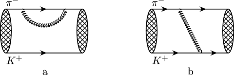
Figure 4: Self-energy (a) and one-photon exchange (b) to the electromagnetic energy shift. The twisted lines denote transverse photons.

The electromagnetic contributions to the energy-level shifts consists of

$$\Delta E^{\rm em}_{nl} = -\frac{1}{8\mu_{+}^{3}}\left(1-\frac{3\mu_{+}}{\Sigma_{+}}\right)\int d^{3}{\bf{r}}\,\Psi^{*}_{nl}({\bf{r}})\Delta^{2}\Psi_{nl}({\bf{r}})+e^{2}\lambda|\Psi_{n0}({\bf{x}}=0)|^{2}$$ (5.6)

$$-\int d\nu({\bf{p}})|\Psi_{nl}({\bf{p}})|^{2}\left[\hat{\Sigma}_{\pi}(\Omega_{n},{\bf{p}})+\hat{\Sigma}_{\scriptscriptstyle K}(\Omega_{n},{\bf{p}})\right]$$

$$-\frac{e^{2}}{M_{\pi^{\scriptscriptstyle{+}}}M_{\scriptscriptstyle{K^{+}}}}\int d\nu({\bf{p}})d\nu({\bf{p}}^{\prime})\Psi_{nl}^{*}({\bf{p}})G_{\gamma}({\bf{p}},{\bf{p}}^{\prime})\Psi_{nl}({\bf{p}}^{\prime}),$$

with $\Omega_{n}=\Sigma_{+}+{\bf{p}}^{2}/(2\mu_{+})-E_{n}$ and $\Psi_{nl}$ denotes the Coulomb wave function for arbitrary $n$ and $l$. Here, the first term contains the mass insertions ${\bf{H}}_{\scriptscriptstyle\rm D}$, the second describes the finite size effects due to ${\bf{H}}_{\lambda}$, while the last two terms come from the self-energy and one-photon exchange diagrams depicted in Figure 4 (a) and (b).

To avoid contributions from hard photon momenta, we use the threshold expansion [55, 56] to evaluate the self-energy contributions. This procedure is outlined in appendix D and the threshold expanded self-energy $\hat{\Sigma}_{h}$, where $h=\pi,K$, is specified in Eq. (D.17). As can be read off from the wave function in momentum space, the relative 3-momentum ${\bf{p}}$ is of order $\delta$. Hence the quantities $\hat{\Sigma}_{\pi}(\Omega_{n},{\bf{p}})$ and $\hat{\Sigma}_{\scriptscriptstyle K}(\Omega_{n},{\bf{p}})$ count as order $\delta^{5}$ and are beyond the accuracy of our calculation.

What remains to be calculated is the one-photon exchange contribution. The integrand

$$G_{\gamma}({\bf{p}},{\bf{p}}^{\prime}) = \frac{1}{|{\bf{p}}-{\bf{p}}^{\prime}|}\left[\frac{\alpha^{2}\mu_{+}}{2n^{2}}+\frac{{\bf{p}}^{2}}{2M_{\pi^{\scriptscriptstyle{+}}}}+\frac{{\bf{p}}^{\prime 2}}{2M_{\scriptscriptstyle{K^{+}}}}+|{\bf{p}}-{\bf{p}}^{\prime}|\right]^{-1}$$ (5.7)

$$\times\frac{1}{4}\left[({\bf{p}}+{\bf{p}}^{\prime})^{2}-\frac{({\bf{p}}^{2}-{{\bf{p}}^{\prime}}^{2})^{2}}{({\bf{p}}-{\bf{p}}^{\prime})^{2}}\right],$$

is a inhomogeneous function in the parameter $\delta$, and to the accuracy we are working required at leading order in $\delta$ only,

$$G_{\gamma}({\bf{p}},{\bf{p}}^{\prime})=\frac{1}{4}\frac{1}{|{\bf{p}}-{\bf{p}}^{\prime}|^{2}}\left[({\bf{p}}+{\bf{p}}^{\prime})^{2}-\frac{({\bf{p}}^{2}-{{\bf{p}}^{\prime}}^{2})^{2}}{({\bf{p}}-{\bf{p}}^{\prime})^{2}}\right]+\cdots$$ (5.8)

In order to evaluate the one-photon exchange contributions, we replace the terms $\sim{\bf{p}}^{2}\Psi^{*}_{nl}({\bf{p}})$ and $\sim{\bf{p^{\prime}}}^{2}\Psi_{nl}({\bf{p^{\prime}}})$ by making use of the Schrödinger equation,

$$\left[{\bf{p}}^{2}+\frac{\alpha^{2}\mu_{+}^{2}}{n^{2}}\right]\Psi_{nl}({\bf{p}})=8\pi\alpha\mu_{+}\int d\nu({\bf{q}})\frac{1}{|{\bf{p}}-{\bf{q}}|^{2}}\Psi_{nl}({\bf{q}}).$$ (5.9)

Further, we use the Fourier transform of $|{\bf{p}}-{\bf{p}}^{\prime}|^{-2}$, $|{\bf{p}}-{\bf{q}}|^{-2}$ and $|{\bf{p}}^{\prime}-{\bf{q}}|^{-2}$ to express the wave functions in coordinate space. The one-photon exchange contribution now reads at order $\alpha^{4}$,

$$\frac{\pi\alpha}{\mu_{+}\Sigma_{+}}|\Psi_{n0}({\bf{x}}=0)|^{2}+\frac{\alpha^{3}\mu_{+}}{n^{2}\Sigma_{+}}\langle r^{-1}\rangle-\frac{3\alpha^{2}}{2\Sigma_{+}}\langle r^{-2}\rangle,$$ (5.10)

where the expectation values are defined as

$$\langle r^{-k}\rangle=\int d^{3}{\bf{r}}\,\Psi^{*}_{nl}({\bf{r}})\frac{1}{|{\bf{r}}|^{k}}\Psi_{nl}({\bf{r}}),\quad k=1,2.$$ (5.11)

The electromagnetic energy shift at order $\alpha^{4}$ yields

$$\Delta E^{\rm em}_{nl} = \frac{\alpha^{4}\mu_{+}}{n^{3}}\left(1-\frac{3\mu_{+}}{\Sigma_{+}}\right)\left[\frac{3}{8n}-\frac{1}{2l+1}\right]+\frac{4\alpha^{4}\mu_{+}^{3}\lambda}{n^{3}}\delta_{l0}$$ (5.12)

$$+\frac{\alpha^{4}\mu_{+}^{2}}{\Sigma_{+}}\left[\frac{1}{n^{3}}\delta_{l0}+\frac{1}{n^{4}}-\frac{3}{n^{3}(2l+1)}\right]+\mathcal{O}(\alpha^{5}{\rm ln}\alpha).$$

Here, the first terms is generated by the mass insertions, the second contains the finite size effects and the last stems from the one-photon exchange contributions (5.10). For $n$ and $l$ arbitrary, we get the same result for the pure QED contributions as Ref. [40, 41, 43]. Further the formula for the ground-state agrees with the result obtained in Ref. [25] for the electromagnetic energy shift of the $\pi^{-}p$ atom, if we replace $\lambda$ through the corresponding quantity in pionic hydrogen.

Figure 5: Annihilation diagram $\pi^{+}\pi^{-}\rightarrow\pi^{+}\pi^{-}$ at order $\alpha$ in the relativistic theory.

To analyze the electromagnetic energy splittings of pionium, we need to construct an effective Lagrangian that describes the relativistic $\pi^{+}\pi^{-}\rightarrow\pi^{+}\pi^{-}$ amplitude at threshold correctly up to and including order $\alpha$. The annihilation graph showed in Figure 5 corresponds to a local four pion interaction in the non-relativistic Lagrangian. However, the corresponding relativistic scattering matrix element vanishes at threshold. We may thus obtain the electromagnetic energy-level shift from Eq. (5.12) by simply substituting $\mu_{+}\rightarrow M_{\pi^{\scriptscriptstyle{+}}}/2$, $\Sigma_{+}\rightarrow 2M_{\pi^{\scriptscriptstyle{+}}}$ and $\lambda\rightarrow 1/3\langle r_{\pi^{+}}^{2}\rangle$,

$$\Delta E^{\rm em}_{\pi,nl}=\alpha^{4}M_{\pi^{\scriptscriptstyle{+}}}\left[\frac{\delta_{l0}}{8n^{3}}+\frac{11}{64n^{4}}-\frac{1}{2n^{3}(2l+1)}\right]+\frac{\alpha^{4}M_{\pi^{\scriptscriptstyle{+}}}^{3}\langle r_{\pi^{+}}^{2}\rangle}{6n^{3}}\delta_{l0}+\mathcal{O}(\alpha^{5}{\rm ln}\alpha).$$ (5.13)

5.2 Decay channels of the $\pi K$ atom

Next we discuss the contributions from other decay channels to the decay width of the $\pi^{-}K^{+}$ atom. As already mentioned in Section 2, for S-states the only possible decay channels are $K^{0}+n_{1}\gamma+n_{2}e^{+}e^{-}$ and $\pi^{0}K^{0}+n_{1}\gamma+n_{2}e^{+}e^{-}$, where $n_{1}+n_{2}>0$. Here $n_{1}$ denotes the number of photons and $n_{2}$ the number of $e^{+}e^{-}$ pairs. The decay widths into $\pi^{-}K^{+}+n_{1}\gamma+n_{2}e^{+}e^{-}$ vanish due to lack of phase space. Moreover, radiative transitions with the emission of one photon are forbidden between two states with $l=0$. For the 2P-state of the $\pi^{-}K^{+}$ atom on the contrary, the main annihilation mechanism is the $2p-1s$ radiative transition into the ground-state, followed by the decay into $\pi^{0}K^{0}$.

To investigate the decays into $K^{0}+n\gamma$, $n=1,2$ we have to extend the Lagrangian in Eqs. (A.4) and (A.5) to include terms with odd intrinsic parity, such as

$$\mathcal{L}_{\rm A}=eD_{1}{\bf{B}}\cdot(\pi_{\scriptscriptstyle{-}}^{\dagger}{\scriptscriptstyle\overleftrightarrow{\textstyle{\bf{D}}}}K_{\scriptscriptstyle{+}}^{\dagger}K_{\scriptscriptstyle{0}}+{\rm h.c})+e^{2}D_{2}{\bf{E}}\cdot{\bf{B}}(\pi_{\scriptscriptstyle{-}}^{\dagger}K_{\scriptscriptstyle{+}}^{\dagger}K_{\scriptscriptstyle{0}}+{\rm h.c})+\cdots,$$ (5.14)

where $u{\scriptscriptstyle\overleftrightarrow{\textstyle{\bf{D}}}}v\doteq u{\bf{D}}v-v{\bf{D}}u$. The covariant derivative ${\bf{D}}$ is specified in appendix A, ${\bf{E}}$ denotes the electric and ${\bf{B}}$ the magnetic field. The couplings $D_{1}$ and $D_{2}$ are real and may be determined through matching with the chiral expansion of the relativistic amplitudes. In the relativistic theory, the $\pi^{+}K^{-}K^{0}2\gamma$ vertex is contained in the Wess-Zumino-Witten term [45]. The $\pi^{+}K^{-}K^{0}\gamma$ interaction occurs not until the odd intrinsic parity sector of the ChPT Lagrangian at $\mathcal{O}(p^{6})$ [46]. The such extended Hamiltonian is hermitian and the operator $\bf\bar{\tau}$ obeys the unitarity condition,

$$\mbox{\boldmath$\bf\bar{\tau}$}(z)-\mbox{\boldmath$\bf\bar{\tau}$}^{\dagger}(z)=-2\pi i\mbox{\boldmath$\bf\bar{\tau}$}(z)\bar{\delta}(z-{\bf{H}}_{0}-{\bf{H}}_{\scriptscriptstyle\rm C})\mbox{\boldmath$\bf\bar{\tau}$}^{\dagger}(z).$$ (5.15)

The symbol $\bar{\delta}$ is understood as follows: in order to evaluate the right-hand side of the equation, we insert a complete set of eigenstates $({\bf{H}}_{0}+{\bf{H}}_{\scriptscriptstyle\rm C})$$\mid\!\beta\rangle=E_{\beta}\mid\!\beta\rangle$, omitting the $n$-th Coulomb eigenstate of the $\pi^{-}K^{+}$ atom. This implies for the total decay width:

$$\Gamma_{nl}=\sum_{\beta}\Gamma_{nl,\beta},$$ (5.16)

where

$$\Gamma_{nl,\beta} = \!\int\!dp_{\beta}\,d\nu({\bf{P}})2\pi\delta(z-E_{\beta})\langle\Psi_{nl},{\bf{P}}\!\mid\mbox{\boldmath$\bf\bar{\tau}$}(z)\mid\!\beta\rangle$$ (5.17)

$$\times\langle\beta\!\mid\mbox{\boldmath$\bf\bar{\tau}$}^{\dagger}(z)\mid\Psi_{nl},{\bf{0}}\rangle,$$

and $z$ is the solution of the master equation (3.10). Here, $dp_{\beta}$ denotes the phase space integral over the intermediate state $|\beta\rangle$. At the accuracy we are considering, we may use $z=E_{n}$. In the following, we estimate the order of the various decays using this formula. As an illustration, we start with the decay into $\pi^{0}K^{0}$. The relative 3-momenta of the $\pi^{-}K^{+}$ pairs ${\bf{p}}$ and ${\bf{p^{\prime}}}$ count as order $\delta$ and we have

$$d\nu({\bf{p}})d\nu({\bf{p}}^{\prime})\Psi_{nl}^{*}({\bf{p}})\Psi_{nl}({\bf{p}}^{\prime})=\mathcal{O}(\delta^{3}).$$ (5.18)

As can be read off from the energy delta function, the outgoing $\pi^{0}$ and $K^{0}$ 3-momenta ${\bf{p}}_{3}$ and ${\bf{p}}_{4}$ count as order $\delta^{1/2}$. This leads to a phase space suppression factor of order $\delta^{1/2}$,

$$d\nu({\bf{p}}_{3})d\nu({\bf{p}}_{4})\delta^{3}({\bf{p}}_{3}+{\bf{p}}_{4})\delta\left(E_{n}-E_{\pi^{0}K^{0}}\right)=\mathcal{O}(\delta^{1/2}),$$ (5.19)

where

$$E_{\pi^{0}K^{0}}=\Sigma_{0}+\frac{{\bf{p}}_{3}^{2}}{2M_{\pi^{\scriptscriptstyle{0}}}}+\frac{{\bf{p}}_{4}^{2}}{2M_{\scriptscriptstyle{K^{0}}}}.$$ (5.20)

Further, the reduced matrix element ${}_{+}\!({\bf{p}}\!\mid\mbox{\boldmath$\bf\bar{\tau}$}(E_{n})\mid\!{\bf{p}}_{3})_{0}$ is of $\mathcal{O}(1)$ and the S-wave decay width thus starts at order $\delta^{7/2}$. The relation (5.17) allows one to rather straightforwardly rederive the next-to-leading order formula for the decay width of the S-states. In order not to interrupt the argument, we relegate the relevant calculation to appendix E, and continue here with the discussion of the radiative decay into $\pi^{0}K^{0}+\gamma$.

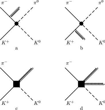
Figure 6: Leading order contributions to the decays into $\pi^{0}K^{0}+\gamma$ and $K^{0}+n\gamma$, $n=1,2$. The dot denotes the coupling $C_{2}$, while the box stands for the couplings $D_{1}$ and $D_{2}$ in $\mathcal{L}_{\rm A}$. The twisted lines denote transverse photons.

The outgoing $\pi^{0}$ and $K^{0}$ 3-momenta again count as $\mathcal{O}(\delta^{1/2})$, while the outgoing photon 3-momentum ${\bf{k}}$ is of order $\delta$. This can by seen by performing the phase space integrations over ${\bf{p}}_{3}$, ${\bf{p}}_{4}$ and ${\bf{k}}$ explicitly. In total, the phase space suppression factor amounts to $\delta^{5/2}$,

$$d\nu({\bf{p}}_{3})d\nu({\bf{p}}_{4})\frac{d^{3}{\bf{k}}}{2\mid\!{\bf{k}}\!\mid}\delta^{3}({\bf{p}}_{3}+{\bf{p}}_{4}+{\bf{k}})\delta\left(E_{n}-E_{\pi^{0}K^{0}\gamma}\right)=\mathcal{O}(\delta^{5/2}),$$ (5.21)

with

$$E_{\pi^{0}K^{0}\gamma}=\Sigma_{0}+\frac{{\bf{p}}_{3}^{2}}{2M_{\pi^{\scriptscriptstyle{0}}}}+\frac{{\bf{p}}_{4}^{2}}{2M_{\scriptscriptstyle{K^{0}}}}+\mid\!{\bf{k}}\!\mid.$$ (5.22)

The leading order contribution stems from Figure 6(a) and 6(b). The corresponding reduced matrix element is given by

$${}_{+}({\bf{p}},-{\bf{p}}\!\mid{\bf{V}}\mbox{\boldmath$\bf\bar{G}$}^{n}_{\rm\scriptscriptstyle C}{\bf{V}}\mid\!{\bf{p}}_{3},{\bf{p}}_{4},{\bf{k}},\lambda)_{0} = -eC_{2}{\bf{p}}\cdot\mbox{\boldmath$\bf\epsilon$}(k,\lambda)\left[f(M_{\pi^{\scriptscriptstyle{+}}},{\bf{p}}^{2},-{\bf{p}}\cdot{\bf{k}})\right.$$ (5.23)

$$+\left.f(M_{\scriptscriptstyle{K^{+}}},{\bf{p}}^{2},{\bf{p}}\cdot{\bf{k}})\right]+\cdots,$$

where

$$f(M,{\bf{p}}^{2},\pm{\bf{p}}\cdot{\bf{k}}) = \frac{1}{M}\left[\frac{\alpha^{2}\mu_{+}}{2n^{2}}+\frac{{\bf{p}}^{2}}{2\mu_{+}}+\frac{{\bf{k}}^{2}}{2M}+\mid\!{\bf{k}}\!\mid\pm\frac{{\bf{p}}\cdot{\bf{k}}}{M}\right]^{-1}.$$ (5.24)

This matrix element is of order $\delta^{1/2}$ which implies that the decay width $\Gamma_{\pi^{0}K^{0}\gamma}$ starts at order $\delta^{13/2}$. However, this contribution vanishes after performing the integrations over ${\bf{p}}$ and ${\bf{p^{\prime}}}$.

Next, we consider the decay into $K^{0}+n\gamma$, $n=1,2$ (see Figure 6(c) and 6(d)). Here, the outgoing $K^{0}$ and photon 3-momenta belong to the hard scale and thus count as $\mathcal{O}(1)$. For $\pi^{-}K^{+}\rightarrow K^{0}+\gamma$, the Lagrangian (5.14) leads to a reduced matrix element of order $\delta^{3/2}$,

$${}_{+}({\bf{p}},-{\bf{p}}\mid{\bf{V}}\mid{\bf{p}}_{4},{\bf{k}},\lambda)_{0}=2eD_{1}{\bf{p}}\cdot\left({\bf{k}}\times\mbox{\boldmath$\bf\epsilon$}(k,\lambda)\right)+\cdots.$$ (5.25)

Naive power counting implies that the decay width into $K^{0}+\gamma$ starts at order $\delta^{6}$. The matrix element (5.25) is odd in ${\bf{p}}$ and the S-wave decay width therefore even more suppressed, while $\Gamma_{n1,K^{0}\gamma}$ starts at order $\delta^{6}$.

For the transition $\pi^{-}K^{+}\rightarrow K^{0}+2\gamma$, we get from the Lagrangian (5.14) a local matrix element of order $\delta$,

$${}_{+}({\bf{p}},-{\bf{p}}\mid{\bf{V}}\mid{\bf{p}}_{4},{\bf{k}}_{1},\lambda_{1},{\bf{k}}_{2},\lambda_{2})_{0} = e^{2}D_{2}k^{0}_{1}\mbox{\boldmath$\bf\epsilon$}(k_{1},\lambda_{1})\cdot\left[{\bf{k}}_{2}\times\mbox{\boldmath$\bf\epsilon$}(k_{2},\lambda_{2})\right]$$ (5.26)

$$-2e^{2}D_{1}\mbox{\boldmath$\bf\epsilon$}(k_{1},\lambda_{1})\cdot\left[{\bf{k}}_{2}\times\mbox{\boldmath$\bf\epsilon$}(k_{2},\lambda_{2})\right]$$

$$+k_{1}\leftrightarrow k_{2},\lambda_{1}\leftrightarrow\lambda_{2},$$

and the decay width of the S-states into $K^{0}+2\gamma$ thus starts at order $\delta^{5}$. For the P-wave decay width into $K^{0}+2\gamma$ this contributions vanishes, because the matrix element in Eq. (5.26) is ${\bf{p}}$ independent.

Processes with a higher number of photons may be treated in a analogous manner. We expect them - using power counting arguments - to be even more suppressed. Since hard processes such as $K^{0}+n_{1}\gamma+n_{2}e^{+}e^{-}$, $n_{1}+n_{2}>0$ do not contribute to the decay width at order $\delta^{9/2}$, we may assume that all couplings in the non-relativistic Lagrangian in Eqs. (A.2), (A.4) and (A.5) are real. The total S-wave decay width of the $\pi^{-}K^{+}$ atom amounts to

$$\Gamma_{n0}=\Gamma_{n0,\pi_{0}K_{0}}+\mathcal{O}(\delta^{5}).$$ (5.27)

The $\pi^{-}K^{+}$ atom in the 2P-state on the other hand decays predominantly through the radiative transition into the ground-state. To evaluate this transition, we insert the ground-state plus one photon into Eq. (5.17). Here the photon 3-momentum ${\bf{k}}$ counts as order $\delta^{2}$, as can be read off from the energy delta function $\delta(E_{2}-E_{1}-|{\bf{k}}|)$. At leading order, we get for the spontaneous $2p-1s$ transition the well-known expression, see e.g. Ref. [57]

$$\Gamma_{21}=\left(\tfrac{2}{3}\right)^{8}\alpha^{5}\mu_{+}+\cdots$$ (5.28)

The result is of order $\alpha^{5}$ and given numerically in Table 3. The first subleading decay mode of the 2P-state starts at order $\delta^{6}$ with the odd intrinsic parity decay into $K^{0}+\gamma$. The P-wave decay width into $\pi^{0}K^{0}$ in Eq. (4.6) is of order $\delta^{13/2}$ and suppressed with respect to radiative $2p-1s$ transition by a factor of $10^{-7}$.

6 Vacuum polarization

What remains to be added are the contributions coming from the electron vacuum polarization. The calculation of these corrections within a non-relativistic Lagrangian approach has been performed in Ref. [22]. In our framework, the contributions due to vacuum polarization arise formally at higher order in $\alpha$. However, they are amplified by powers of the coefficient $\mu_{+}/m_{e}$, where $m_{e}$ denotes the electron mass. To the accuracy considered here, the only effect of the vacuum polarization of the electron is a modification of the Coulomb potential ${\bf{H}}_{\scriptscriptstyle\rm C}\rightarrow{\bf{H}}_{\scriptscriptstyle\rm C}+{\bf{H}}_{\rm vac}$, with

$${}_{+}({\bf{p}}\!\mid{\bf{H}}_{\rm vac}\mid\!{\bf{q}})_{+}=-\frac{4\alpha^{2}}{3}\int_{4m_{e}^{2}}^{\infty}\frac{ds}{s+({\bf{p}}-{\bf{q}})^{2}}\frac{1}{s}\left[1+\frac{2m_{e}^{2}}{s}\right]\left[1-\frac{4m_{e}^{2}}{s}\right]^{1/2}.$$ (6.1)

The vacuum polarization leads to an electromagnetic energy shift evaluated in Refs. [22, 25, 44],

$$\Delta E^{\rm vac}_{nl}=\left(\Psi_{nl}\!\mid{\bf{H}}_{\rm vac}\mid\!\Psi_{nl}\right).$$ (6.2)

For the first two energy-level shifts of pionium and the $\pi^{\pm}K^{\mp}$ atom, $\Delta E^{\rm vac}_{\pi,nl}$ and $\Delta E^{\rm vac}_{nl}$ are given numerically in Table 2 and 3. Formally of order $\alpha^{2l+5}$, this contribution is numerically sizeable due to its large coefficient containing $(\mu_{+}/m_{e})^{2l+2}$.

The vacuum polarization also interferes with strong interactions and contributes to the decay width and to the strong energy shift. This can be seen by inserting the modified Coulomb potential into the master equation (3.10). For the spectrum and the width of the $\pi^{\pm}K^{\mp}$ atom, we get

$$\Gamma_{n0} = \frac{8\alpha^{3}\mu_{+}^{2}}{n^{3}}p_{n}^{*}(a_{0}^{-})^{2}\left(1+\delta_{{\scriptscriptstyle K},n}+\delta^{\rm vac}_{{\scriptscriptstyle K},n}\right),$$

$$\Delta E_{n0}^{\rm h} = -\frac{2\alpha^{3}\mu_{+}^{2}}{n^{3}}(a_{0}^{+}+a_{0}^{-})\left(1+\delta_{{\scriptscriptstyle K},n}^{\prime}+\delta^{\rm vac}_{{\scriptscriptstyle K},n}\right).$$ (6.3)

What concerns pionium, the decay width and strong energy shift are modified, according to

$$\Gamma_{\pi,n0} = \frac{2\alpha^{3}}{9n^{3}}p_{\pi,n}^{*}(a_{0}^{0}-a_{0}^{2})^{2}\left(1+\delta_{\pi,n}+\delta^{\rm vac}_{\pi,n}\right),$$

$$\Delta E_{\pi,n0}^{\rm h} = -\frac{\alpha^{3}M_{\pi^{\scriptscriptstyle{+}}}}{6n^{3}}(2a_{0}^{0}+a_{0}^{2})\left(1+\delta_{\pi,n}^{\prime}+\delta^{\rm vac}_{\pi,n}\right).$$ (6.4)

The correction $\delta^{\rm vac}_{h,n}$, $h=\pi,K$ is proportional to the change in the Coulomb wave function [22] of the bound system due to vacuum polarization,

$$\delta^{\rm vac}_{h,n}=\frac{2\delta\Psi_{n0}({\bf{x}}=0)}{\Psi_{n0}({\bf{x}}=0)}.$$ (6.5)

Here, $\Psi_{nl}$ stands for a generic Coulomb wave function and $h=\pi,K$. For the ground-state, this result is contained in Table II of Ref. [22]. Formally, $\delta^{\rm vac}_{h,n}$ is of order $\alpha^{2}$, but enhanced because of the large coefficient containing $\mu_{+}/m_{e}$.

7 Numerics

	$10^{2}\delta_{h,1}$	$10^{2}\delta_{h,2}$	$10^{2}\delta_{h,1}^{\prime}$	$10^{2}\delta_{h,2}^{\prime}$
$\pi^{+}\pi^{-}$ atom	$5.8\pm 1.2$	$5.6\pm 1.2$	$6.2\pm 1.2$	$6.1\pm 1.2$
$\pi^{\pm}K^{\mp}$ atom	$4.0\pm 2.2$	$3.8\pm 2.2$	$1.7\pm 2.2$	$1.5\pm 2.2$

Table 1: Next-to-leading order corrections to the Deser-type formulae.

In the numerical evaluation of the widths and energy shifts of the $\pi^{+}\pi^{-}$ and $\pi^{\pm}K^{\mp}$ atoms, we use the following numbers: The $\pi\pi$ scattering lengths yield $a_{0}^{0}=0.220\pm 0.005$, $a_{0}^{2}=-0.0444\pm 0.0010$ and $a_{1}^{1}=(0.379\pm 0.005)\cdot 10^{-1}M_{\pi^{\scriptscriptstyle{+}}}^{-2}$ [4, 5]. The correlation matrix for $a_{0}^{0}$ and $a_{0}^{2}$ is given in Ref. [5]. For the isospin symmetry breaking corrections to the $\pi\pi$ threshold amplitudes (4.14) and (4.17) at order $e^{2}p^{2}$, we use $\epsilon_{\pi}=(0.61\pm 0.16)\cdot 10^{-2}$ and $\epsilon_{\pi}^{\prime}=(0.37\pm 0.08)\cdot 10^{-2}$ [23, 54]. The values for the $\pi K$ scattering lengths are taken from the recent analysis of data and Roy-Steiner equations [33]. The S-wave scattering lengths yield $a_{0}^{+}=(0.045\pm 0.012)M_{\pi^{\scriptscriptstyle{+}}}^{-1}$, $a_{0}^{-}=(0.090\pm 0.005)M_{\pi^{\scriptscriptstyle{+}}}^{-1}$[33], and for the P-waves we use $a_{1}^{1/2}=(0.19\pm 0.01)\cdot 10^{-1}M_{\pi^{\scriptscriptstyle{+}}}^{-3}$ and $a_{1}^{3/2}=(0.65\pm 0.44)\cdot 10^{-3}M_{\pi^{\scriptscriptstyle{+}}}^{-3}$[33]. The correlation parameter for $a_{0}^{+}$ and $a_{0}^{-}$ is also given in Ref. [33]. The isospin breaking corrections to the $\pi K$ threshold amplitudes (4.4) and (4.9) have been worked out in Refs. [36, 50, 51] at $\mathcal{O}(p^{4},e^{2}p^{2})$. Whereas the analytic expressions for $\epsilon$ and $\epsilon^{\prime}$ obtained in Refs. [36, 50, 51] are not identical, the numerical values agree within the uncertainties quoted in [51]. In the following, we use [51] $\epsilon=(0.1\pm 0.1)\cdot 10^{-2}M_{\pi^{+}}^{-1}$ and $\epsilon^{\prime}=(0.1\pm 0.3)\cdot 10^{-2}M_{\pi^{+}}^{-1}$. For the charge radii of the pion and kaon, we take $\langle r^{2}_{\pi^{+}}\rangle=(0.452\pm 0.013)\,{\rm fm^{2}}$ and $\langle r^{2}_{\scriptscriptstyle K^{+}}\rangle=(0.363\pm 0.072)\,{\rm fm^{2}}$ [58]. In the evaluation of the uncertainties, we take into account the correlation between the $\pi\pi$, ($\pi K$) scattering lengths.

The isospin breaking corrections $\delta_{h,n}$ and $\delta_{h,n}^{\prime}$, $h=\pi,K$ to the widths (4.5), (4.16) and strong energy shifts (4.10), (4.18) are listed in Table 1. The energy shift corrections $\delta_{{\scriptscriptstyle K},n}^{\prime}$ are smaller than in the case of pionium. This discrepancy comes from the different size of the isospin breaking contributions to the elastic one-particle irreducible $\pi\pi$ and $\pi K$ amplitudes. At leading order in the chiral expansion, the isospin breaking part of the $\pi^{-}K^{+}\rightarrow\pi^{-}K^{+}$ amplitude at threshold is suppressed by a factor of $M_{\pi^{\scriptscriptstyle{+}}}/M_{\scriptscriptstyle{K^{+}}}$ with respect to the corresponding quantity in $\pi\pi$ scattering.

As described in Section 6, Eqs. (6.3) and (6.4), the width and strong energy shift are modified due to vacuum polarization, according to

$$\delta_{h,n}\rightarrow\delta_{h,n}+\delta_{h,n}^{\rm vac},\quad\delta_{h,n}^{\prime}\rightarrow\delta_{h,n}^{\prime}+\delta_{h,n}^{\rm vac},$$ (7.1)

where $h=\pi,K$ and $\delta_{h,n}^{\rm vac}$ is defined in Eq. (6.5). For the ground-state, the corrections due to vacuum polarization yield $\delta^{\rm vac}_{{\scriptscriptstyle K},1}=0.45\cdot 10^{-2}$ and $\delta^{\rm vac}_{\pi,1}=0.31\cdot 10^{-2}$[22]. However, for the numerical analysis of the width and the strong energy shift, we may neglect the contributions from $\delta^{\rm vac}_{h,n}$, because the uncertainties in $\delta_{h,n}$ and $\delta_{h,n}^{\prime}$ are larger than $\delta^{\rm vac}_{h,n}$ itself.

$\pi^{+}\pi^{-}$ atom	$\Delta E^{\rm em}_{\pi,nl}$[eV]	$\Delta E^{\rm vac}_{\pi,nl}$[eV]	$\Delta E^{\rm h}_{\pi,nl}$[eV]	$10^{15}\tau_{\pi,nl}$[s]
$n$=1, $l$=0	$-0.065$	$-0.942$	$-3.8\pm 0.1$	$2.9\pm 0.1$
$n$=2, $l$=0	$-0.012$	$-0.111$	$-0.47\pm 0.01$	$23.3\pm 0.7$
$n$=2, $l$=1	$-0.004$	$-0.004$	$\simeq-1\cdot 10^{-6}$	$\simeq 1.2\cdot 10^{4}$

Table 2: Numerical values for the energy shift and the lifetime of the $\pi^{+}\pi^{-}$ atom.

$\pi^{\pm}K^{\mp}$ atom	$\Delta E^{\rm em}_{nl}$[eV]	$\Delta E^{\rm vac}_{nl}$[eV]	$\Delta E^{\rm h}_{nl}$[eV]	$10^{15}\tau_{nl}$[s]
$n$=1, $l$=0	$-0.095$	$-2.56$	$-9.0\pm 1.1$	$3.7\pm 0.4$
$n$=2, $l$=0	$-0.019$	$-0.29$	$-1.1\pm 0.1$	$29.4\pm 3.3$
$n$=2, $l$=1	$-0.006$	$-0.02$	$\simeq-3\cdot 10^{-6}$	$\simeq 0.7\cdot 10^{4}$

Table 3: Numerical values for the energy shift and the lifetime of the $\pi^{\pm}K^{\mp}$ atom.

For the first two states of the $\pi^{+}\pi^{-}$ and $\pi^{\pm}K^{\mp}$ atoms, the numerical values for the lifetime $\tau_{nl}\doteq\Gamma^{-1}_{nl}$, ($\tau_{\pi,nl}\doteq\Gamma^{-1}_{\pi,nl}$) and the energy shifts are listed in Table 2 and 3. The numbers for the lifetime and strong energy shifts of the S-states are valid at next-to-leading order in isospin symmetry breaking. The bulk part in the uncertainties of these quantities is due to the uncertainties in the corresponding scattering lengths. For the lifetime of the 2P-state, the numerical values are valid at leading order only, and determined by the $2p-1s$ radiative transition in Eq. (5.28) [59].

The energy-level shift due to vacuum polarization $\Delta E^{\rm vac}_{nl}$, ($\Delta E^{\rm vac}_{\pi,nl}$) [22, 44] is specified in Eq. (6.2). Formally of higher order in $\alpha$, this contribution is numerically sizable. We do not display the error bars for the electromagnetic energy shifts. At order $\alpha^{4}$, they come from the uncertainties in the charge radii of the pion and kaon only. In the case of pionium, the uncertainties of $\Delta E_{\pi,10}^{\rm em}$ at order $\alpha^{4}$ amount to about $0.7\%$, while for the $\pi^{\pm}K^{\mp}$ atom $\Delta E_{10}^{\rm em}$ is known at the $5\%$ level. To estimate the order of magnitude of the electromagnetic corrections at higher order, we may compare with positronium. Here, the $\alpha^{5}$ and $\alpha^{5}\,{\rm ln}\alpha$ corrections [60] amount to about $2\%$ with respect to the $\alpha^{4}$ contributions.

Both, the electromagnetic and vacuum polarization contributions to the energy shift are known to a high accuracy. A future precision measurement of the energy splitting between the $n$S and $n$P states [61] will therefore allow one to extract the strong S-wave energy shift in Eq. (4.10), and to determine the combination $a_{0}^{+}+a_{0}^{-}$ of the $\pi K$ scattering lengths. The $2s-2p$ energy splitting yields

$$\Delta E_{2s-2p} = \Delta E_{20}^{\rm h}+\Delta E_{20}^{\rm em}-\Delta E_{21}^{\rm em}+\Delta E_{20}^{\rm vac}-\Delta E_{21}^{\rm vac}$$ (7.2)

$$= -1.4\pm 0.1\,{\rm eV}.$$

The uncertainty displayed is the one in $\Delta E_{2}^{\rm h}$ only. To the accuracy we are working, we may neglect the strong shift in the $2$P state, it is suppressed by the power of $\alpha^{5}$. For pionium the energy splitting between the 2S and 2P states reads

$$\Delta E_{\pi,2s-2p} = \Delta E_{\pi,20}^{\rm h}+\Delta E_{\pi,20}^{\rm em}-\Delta E_{\pi,21}^{\rm em}+\Delta E_{\pi,20}^{\rm vac}-\Delta E_{\pi,21}^{\rm vac}$$ (7.3)

$$= -0.59\pm 0.01\,{\rm eV}.$$

Again the uncertainty displayed is the one in $\Delta E_{\pi,2}^{\rm h}$ only and we may neglect contributions from the strong shift in the $2$P state.

As an illustration, we alternatively use the ChPT predictions for the $\pi K$ scattering lengths [34, 36] in the numerical evaluation of the lifetime. The ChPT predictions yield at order $p^{4}$, $a_{0}^{+}=(0.032\pm 0.016)M_{\pi^{\scriptscriptstyle{+}}}^{-1}$ and $a_{0}^{-}=(0.079\pm 0.001)M_{\pi^{\scriptscriptstyle{+}}}^{-1}$ [33]. Here, the errors include the uncertainties in the values of the input parameters only. The uncertainty in $a_{0}^{-}$ is remarkably small, because the isospin odd scattering length involves at $\mathcal{O}(p^{4})$ a single low–energy constant $L_{5}^{r}$ [36]. On the other hand, $a_{0}^{+}$ contains apart from the combination $2L_{6}^{r}+L_{8}^{r}$ five further coupling constants [36], which are enhanced by one power of $M_{\scriptscriptstyle{K^{+}}}/M_{\pi^{\scriptscriptstyle{+}}}$ with respect to the counterterm in $a_{0}^{-}$. For $a_{0}^{-}$, the two-loop correction has to be rather substantial, in order to reproduce the central value of the Roy-Steiner evaluation. Very recently, the chiral expansion of the $\pi K$ scattering amplitude at next-to-next-to-leading order became available [37]. According to the preliminary numerical study performed in Ref. [37], the S-wave scattering lengths are at order $p^{6}$ in reasonable agreement with the Roy-Steiner evaluation [33]. The $\mathcal{O}(p^{4})$ ChPT prediction for the lifetime of the $\pi^{\pm}K^{\mp}$ atom in its ground-state is

$$\tau_{10}=4.7\cdot 10^{-15}{\rm s},\quad\textrm{ChPT},[\mathcal{O}(p^{4})],$$ (7.4)

whereas

$$\tau_{10}=(3.7\pm 0.4)\cdot 10^{-15}{\rm s},\quad\textrm{Roy-Steiner}.$$ (7.5)

The ChPT prediction is valid at next-to-leading order in isospin symmetry breaking and up to and including $\mathcal{O}(p^{4})$ in the chiral expansion.

8 Summary and Outlook

We have considered the spectra and decays of $\pi^{+}\pi^{-}$ and $\pi^{\pm}K^{\mp}$ atoms in the framework of QCD $+$ QED. We evaluated the corrections to the Deser-type formulae for the width and the energy shift - valid at next-to-leading order in isospin symmetry breaking - within a non-relativistic effective field theory. It is convenient to introduce a different book keeping for the $\pi^{+}\pi^{-}$ and $\pi^{\pm}K^{\mp}$ atoms. What concerns pionium, we count $\alpha$ and $(m_{u}-m_{d})^{2}$ as small quantities of order $\delta$, in the case of the $\pi^{\pm}K^{\mp}$ atom both $\alpha$ and $m_{u}-m_{d}$ are of order $\delta$. The different counting schemes are due to the fact that in QCD, the pion mass difference starts at $(m_{u}-m_{d})^{2}$, while the kaon mass difference is linear in $m_{u}-m_{d}$.

Consider first the energy shifts that are split into an electromagnetic and a strong part, according to Eq. (2.1). The electromagnetic part in Eqs. (5.12) and (5.13) contains both pure QED contributions as well as finite size effects due to the charge radii of the pion and kaon. The strong energy shift of the $\pi^{-}K^{+}$ atom is proportional to the one-particle irreducible $\pi^{-}K^{+}\rightarrow\pi^{-}K^{+}$ scattering amplitude at threshold. In the isospin symmetry limit, the elastic threshold amplitude reduces to the sum of isospin even and odd scattering lengths $a_{0}^{+}+a_{0}^{-}$. The isospin breaking contributions to the amplitude have been evaluated at $\mathcal{O}(e^{2}p^{2},p^{4})$[36, 51] in the framework of ChPT. The result in Eq. (4.10) displays the S-wave energy shift in terms of the sum $a_{0}^{+}+a_{0}^{-}$, and a correction of order $\alpha$ and $m_{u}-m_{d}$. For the first two energy-level shifts, the isospin symmetry breaking correction modifies the leading order term at the $2\%$ level. The isospin even scattering length $a_{0}^{+}$ is sensitive to the combination of low–energy constants $2L_{6}^{r}+L_{8}^{r}$. The consequences of this observation for the SU(3)$\times$SU(3) quark condensate [39] remain to be worked out. In the case of pionium, the strong energy shift displayed in Eq. (4.18) is related to the $\pi\pi$ scattering lengths combination $2a_{0}^{0}+a_{0}^{2}$ and a correction of order $\alpha$ and $(m_{u}-m_{d})^{2}$. For the first two energy-levels, these isospin symmetry breaking contributions amount to about $6\%$.

A future measurement of the energy splitting between the $2$S and $2$P state in the $\pi^{+}\pi^{-}$, ($\pi^{\pm}K^{\mp}$) atom will allow one to extract the strong energy shift and to determine the scattering lengths combination $2a_{0}^{0}+a_{0}^{2}$, ($a_{0}^{+}+a_{0}^{-}$). This is due to the fact that the electromagnetic energy shifts are known to high accuracy and the strong P-wave energy shifts in Eqs. (4.12) and (4.19) are suppressed by the power of $\alpha^{5}$. However, another higher order correction - generated by the vacuum polarization - is numerically sizable and contributes to the energy splitting in Eqs. (7.2) and (7.3). Formally of order $\alpha^{2l+5}$, this correction is enhanced due to its large coefficient containing $(\mu_{+}/m_{e})^{2l+2}$.

We now turn to the decay widths of the $\pi^{+}\pi^{-}$ and $\pi^{-}K^{+}$ atoms. At leading and next-to leading order the $\pi^{+}\pi^{-}$ and $\pi^{-}K^{+}$ atoms decay into $2\pi^{0}$ and $\pi^{0}K^{0}$ exclusively. Aside from a kinematical factor - the relativistic outgoing 3-momentum of the bound system - their decay width can be expanded in powers of $\alpha$ and $m_{u}-m_{d}$. By invoking ChPT, the result for the S-wave decay width of the $\pi^{-}K^{+}$ atom may be expressed in terms of the isospin odd scattering length $a_{0}^{-}$, and an isospin symmetry breaking correction of order $\alpha$ and $m_{u}-m_{d}$, see Eq. (4.5). For the ground-state decay width, this correction modifies the leading order Deser-type relation at the $4\%$ level. The next-to-leading order result for the S-wave decay width of pionium is given in Eq. (4.16). The expression for the ground-state width agrees with the result obtained in Refs. [20, 23, 30].

For the 2P state of the $\pi^{-}K^{+}$, ($\pi^{+}\pi^{-}$) atom, the decay width starts at order $\alpha^{5}$ with the $2p-1s$ radiative transition into the ground-state, see Eq. (5.28). The P-wave decay width of the $\pi^{-}K^{+}$ atom into $\pi^{0}K^{0}$ in Eq. (4.6) is suppressed by the power of $\delta^{13/2}$. For pionium, the P-wave decay width into a pair of two neutral pions vanishes due to $C$ invariance.

We find it very exciting that in view to the beautiful work performed by our experimental colleagues, we may expect that many of the above predictions will be confronted with experimental data in a not too distant future. This will certainly improve our knowledge of the low–energy structure of QCD.

Appendix A Non-relativistic Lagrangian

The non-relativistic Lagrangian must be invariant under space rotation, $P$, $T$ and gauge transformations. We do not include terms corresponding to transitions between sectors with different numbers of heavy fields (pions and kaons). These interactions describe processes with an energy release at the hard scale. In general, such decay processes are accounted for by introducing complex couplings in the non-relativistic Lagrangian. However, as shown in Section 5.2, intermediate states do not contribute to the decay width at order $\delta^{9/2}$ and we may therefore assume the low–energy couplings to be real.

In the sector with one or two mesons, the non-relativistic effective Lagrangian is given by

$$\mathcal{L}_{\scriptscriptstyle\rm NR}=\mathcal{L}_{1}+\mathcal{L}_{2}^{(0)}+\mathcal{L}_{2}^{(2)}+\cdots$$ (A.1)

The first term contains the one-pion and one-kaon sectors

$$\mathcal{L}_{1} = \frac{1}{2}({\bf{E}}^{2}-{\bf{B}}^{2})+\pi_{\scriptscriptstyle{0}}^{\dagger}\Big{(}i\partial_{t}-M_{\pi^{\scriptscriptstyle{0}}}+\frac{\Delta}{2M_{\pi^{\scriptscriptstyle{0}}}}+\frac{\Delta^{2}}{8M_{\pi^{\scriptscriptstyle{0}}}^{3}}+\cdots\Big{)}\pi_{\scriptscriptstyle{0}}$$ (A.2)

$$+K_{\scriptscriptstyle{0}}^{\dagger}\Big{(}i\partial_{t}-M_{\scriptscriptstyle{K^{0}}}+\frac{\Delta}{2M_{\scriptscriptstyle{K^{0}}}}+\frac{\Delta^{2}}{8M_{\scriptscriptstyle{K^{0}}}^{3}}+\cdots\Big{)}K_{\scriptscriptstyle{0}}$$

$$+\sum_{\pm}\pi_{\pm}^{\dagger}\Big{(}iD_{t}-M_{\pi^{\scriptscriptstyle{+}}}+\frac{{\bf{D}}^{2}}{2M_{\pi^{\scriptscriptstyle{+}}}}+\frac{{\bf{D}}^{4}}{8M_{\pi^{\scriptscriptstyle{+}}}^{3}}+\cdots\Big{)}\pi_{\pm}$$

$$+\sum_{\pm}K_{\pm}^{\dagger}\Big{(}iD_{t}-M_{\scriptscriptstyle{K^{+}}}+\frac{{\bf{D}}^{2}}{2M_{\scriptscriptstyle{K^{+}}}}+\frac{{\bf{D}}^{4}}{8M_{\scriptscriptstyle{K^{+}}}^{3}}+\cdots\Big{)}K_{\pm}$$

$$\mp e\sum_{\pm}{\bf{D}}({\bf{E}})\left(\frac{c_{\pi}}{6M_{\pi^{\scriptscriptstyle{+}}}^{2}}\pi_{\pm}^{\dagger}\pi_{\pm}+\frac{c_{\scriptscriptstyle K}}{6M_{\scriptscriptstyle{K^{+}}}^{2}}K_{\pm}^{\dagger}K_{\pm}+\cdots\right),$$

with electromagnetic charge $e$, ${\bf{E}}=-\nabla A_{0}-\dot{{\bf{A}}}$ and ${\bf{B}}=\nabla\times{\bf{A}}$. The covariant derivatives of the charged meson fields are given by

$$D_{t}\pi_{\pm}=\partial_{t}\pi_{\pm}\mp ieA_{0}\pi_{\pm},\quad{\bf{D}}\pi_{\pm}=\nabla\pi_{\pm}\pm ie{\bf{A}}\pi_{\pm},$$

$$D_{t}K_{\pm}=\partial_{t}K_{\pm}\mp ieA_{0}K_{\pm},\quad{\bf{D}}K_{\pm}=\nabla K_{\pm}\pm ie{\bf{A}}K_{\pm}.$$ (A.3)

The one-pion-one-kaon sector of total zero charge reads at lowest order

$$\mathcal{L}_{2}^{(0)} = C_{1}\pi_{\scriptscriptstyle{-}}^{\dagger}K_{\scriptscriptstyle{+}}^{\dagger}\pi_{\scriptscriptstyle{-}}K_{\scriptscriptstyle{+}}+C_{2}\left(\pi_{\scriptscriptstyle{-}}^{\dagger}K_{\scriptscriptstyle{+}}^{\dagger}\pi_{\scriptscriptstyle{0}}K_{\scriptscriptstyle{0}}+\textrm{h.c}\right)+C_{3}\pi_{\scriptscriptstyle{0}}^{\dagger}K_{\scriptscriptstyle{0}}^{\dagger}\pi_{\scriptscriptstyle{0}}K_{\scriptscriptstyle{0}}.$$ (A.4)

To evaluate the decay width and energy shifts of the $\pi^{-}K^{+}$ atom, we need in addition the following terms with two covariant space derivatives

$$\mathcal{L}_{2}^{(2)} = C_{4}\left(\pi_{\scriptscriptstyle{-}}^{\dagger}{\scriptscriptstyle\overleftrightarrow{\textstyle{\bf{D}}}}^{2}K_{\scriptscriptstyle{+}}^{\dagger}\pi_{\scriptscriptstyle{0}}K_{\scriptscriptstyle{0}}+\textrm{h.c}\right)+C_{5}\left(\pi_{\scriptscriptstyle{-}}^{\dagger}{\scriptscriptstyle\overleftrightarrow{\textstyle{\bf{D}}}}^{2}K_{\scriptscriptstyle{+}}^{\dagger}\pi_{\scriptscriptstyle{-}}K_{\scriptscriptstyle{+}}+{\rm h.c}\right)$$ (A.5)

$$+C_{6}(\pi_{\scriptscriptstyle{-}}^{\dagger}\pi_{\scriptscriptstyle{-}}){\bf{D}}^{2}(K_{\scriptscriptstyle{+}}^{\dagger}K_{\scriptscriptstyle{+}})+C_{7}\left(\nabla\pi_{\scriptscriptstyle{-}}^{\dagger}K_{\scriptscriptstyle{+}}^{\dagger}\nabla\pi_{\scriptscriptstyle{0}}K_{\scriptscriptstyle{0}}+\textrm{h.c}\right)+\cdots,$$

where $u{\scriptscriptstyle\overleftrightarrow{\textstyle{\bf{D}}}}^{2}v\doteq u{\bf{D}}^{2}v+v{\bf{D}}^{2}u$. We work in the center of mass system and thus omit terms proportional to the c.m. momentum. We do not display time derivatives, for on-shell matrices they can be eliminated by the use of the equations of motion. The parameters $M_{\pi^{i}}$ ($M_{K^{i}}$) denote the physical pion, (kaon) masses – there is no mass renormalization in the non-relativistic theory, see Section 3.3.

We work in the Coulomb gauge and eliminate the $A^{0}$ component of the photon field by the use of the equations of motion. At the accuracy we are considering, the term linear in ${\bf{D}}({\bf{E}})$ in Eq. (A.2) then reduces to a local interaction which modifies the low–energy coupling $C_{1}$,

$$C_{1}^{\prime} = C_{1}-e^{2}\lambda,$$

$$\lambda = \frac{c_{\pi}}{6M_{\pi^{\scriptscriptstyle{+}}}^{2}}+\frac{c_{\scriptscriptstyle K}}{6M_{\scriptscriptstyle{K^{+}}}^{2}}.$$ (A.6)

It is sufficient to match the non-relativistic couplings $c_{\pi}$ and $c_{\scriptscriptstyle K}$ at order $\delta^{0}$. We therefore consider the pion and kaon electromagnetic form-factors in the external field $A_{\mu}$. The results of the matching yield

$$c_{\pi}=M_{\pi^{\scriptscriptstyle{+}}}^{2}\langle r^{2}_{\pi}\rangle,\quad c_{\scriptscriptstyle K}=M_{\scriptscriptstyle{K^{+}}}^{2}\langle r^{2}_{\scriptscriptstyle K}\rangle,$$ (A.7)

where $r_{\pi}$ and $r_{\scriptscriptstyle K}$ denote the charge radii of the charged pion and kaon, respectively. The remaining low energy constants $C_{i}$, $i=1,\dots 7$ may be determined through matching the $\pi K$ amplitude in the vicinity of the threshold for different channels, see Section 3.3.

Appendix B Relativistic scattering amplitudes

First, we consider the $S=1$ processes

$$\pi^{-}K^{+}\rightarrow\pi^{-}K^{+},\quad\pi^{-}K^{+}\rightarrow\pi^{0}K^{0},\quad\pi^{0}K^{0}\rightarrow\pi^{0}K^{0},$$ (B.1)

in the isospin symmetry limit. The decomposition into amplitudes with definite isospin yields

$$T^{\pm;\pm} = \frac{1}{3}\left[T^{\scriptscriptstyle 3/2}(s,t)+2T^{\scriptscriptstyle 1/2}(s,t)\right],$$

$$T^{00;\pm} = \frac{\sqrt{2}}{3}\left[T^{\scriptscriptstyle 3/2}(s,t)-T^{\scriptscriptstyle 1/2}(s,t)\right],$$

$$T^{00;00} = \frac{1}{3}\left[2T^{\scriptscriptstyle 3/2}(s,t)+T^{\scriptscriptstyle 1/2}(s,t)\right].$$ (B.2)

The isospin $I=1/2$ and $I=3/2$ components are related via

$$T^{\scriptscriptstyle 1/2}(s,t,u)=\frac{3}{2}T^{\scriptscriptstyle 3/2}(u,t,s)-\frac{1}{2}T^{\scriptscriptstyle 3/2}(s,t,u).$$ (B.3)

The $T^{+}$, ($T^{-}$) amplitude

$$T^{+}(s,t) = \frac{1}{3}\left[T^{\scriptscriptstyle 1/2}(s,t)+2T^{\scriptscriptstyle 3/2}(s,t)\right],$$

$$T^{-}(s,t) = \frac{1}{3}\left[T^{\scriptscriptstyle 1/2}(s,t)-T^{\scriptscriptstyle 3/2}(s,t)\right],$$ (B.4)

is even (odd) under $s\leftrightarrow u$ crossing. In the s-channel, the decomposition into partial waves reads

$$T^{I}(s,t)=16\pi\sum_{l=0}^{\infty}(2l+1)t^{I}_{l}(s)P_{l}({\rm cos}\,\theta),$$ (B.5)

where $s=[\omega_{\pi^{+}}({\bf{p}})+\omega_{K^{+}}({\bf{p}})]^{2}$, $t=-2{\bf{p}}^{2}(1-{\rm cos}\,\theta)$ and $\theta$ is the scattering angle in the c.m. system.

The real part of the partial wave amplitudes near threshold is of the form,

$${\rm Re}\,t^{I}_{l}(s)=\frac{\sqrt{s}}{2}{\bf{p}}^{2l}\left(a^{I}_{l}+b^{I}_{l}{\bf{p}}^{2}+\mathcal{O}({\bf{p}}^{4})\right),$$ (B.6)

where $a^{I}_{l}$ denote the scattering lengths and $b^{I}_{l}$ the effective ranges.

What follows, are the $\pi\pi$ scattering processes:

$$\pi^{-}\pi^{+}\rightarrow\pi^{-}\pi^{+},\quad\pi^{-}\pi^{+}\rightarrow\pi^{0}\pi^{0},$$ (B.7)

with

$$T^{\pm;\pm}_{\pi} = \frac{1}{6}\left[T^{2}_{\pi}(s,t)+3T^{1}_{\pi}(s,t)+2T^{0}_{\pi}(s,t)\right],$$

$$T^{00;\pm}_{\pi} = \frac{1}{3}\left[T^{2}_{\pi}(s,t)-T^{0}_{\pi}(s,t)\right].$$ (B.8)

The decomposition into partial waves yields

$$T^{I}_{\pi}(s,t)=32\pi\sum_{l=0}^{\infty}(2l+1)P_{l}({\rm cos}\,\theta)t^{I}_{\pi,l}(s),$$ (B.9)

where $s=4(M_{\pi^{\scriptscriptstyle{+}}}^{2}+{\bf{p}}^{2})$. At threshold, the partial wave amplitudes take the form

$${\rm Re}t_{\pi,l}^{I}(s)={\bf{p}}^{2l}\left[a_{l}^{I}+{\bf{p}}^{2}b_{l}^{I}+\mathcal{O}({\bf{p}}^{4})\right].$$ (B.10)

Appendix C Schwinger’s Green function

The Schwinger Green function fulfills

$$\left[E-\frac{{\bf{q}}^{2}}{2\mu_{+}}\right]{}_{+}\!({\bf{q}}\!\mid{\bf{G}}_{\scriptscriptstyle\rm C}(z)\mid\!{\bf{p}})_{+}+e^{2}\int d\nu(k)\frac{1}{({\bf{k}}-{\bf{q}})^{2}}{}_{+}\!({\bf{k}}\!\mid{\bf{G}}_{\scriptscriptstyle\rm C}(z)\mid\!{\bf{p}})_{+}=$$

$$(2\pi)^{3}\delta^{3}({\bf{q}}-{\bf{p}}),$$ (C.1)

where $E=z-\Sigma_{+}$. The explicit expression is given by

$${}_{+}\!({\bf{q}}\!\mid{\bf{G}}_{\scriptscriptstyle\rm C}(z)\mid\!{\bf{p}})_{+} = \frac{(2\pi)^{3}\delta^{3}({\bf{q}}-{\bf{p}})}{E-\frac{{\bf{q}}^{2}}{2\mu_{+}}}-\frac{1}{E-\frac{{\bf{q}}^{2}}{2\mu_{+}}}\frac{4\pi\alpha}{({\bf{q}}-{\bf{p}})^{2}}\frac{1}{E-\frac{{\bf{p}}^{2}}{2\mu_{+}}}$$ (C.2)

$$-\frac{1}{E-\frac{{\bf{q}}^{2}}{2\mu_{+}}}4\pi\alpha\eta I(E,{\bf{q}},{\bf{p}})\frac{1}{E-\frac{{\bf{p}}^{2}}{2\mu_{+}}},$$

with $\eta=\alpha/2(-E/(2\mu_{+}))^{-1/2}$. The function

$$I(E,{\bf{q}},{\bf{p}})=\int_{0}^{1}d{\bf{\rho}}\,\rho^{-\eta}\left[({\bf{q}}-{\bf{p}})^{2}\rho+\frac{\eta^{2}}{\alpha^{2}}(1-\rho^{2})(E-\frac{{\bf{q}}^{2}}{2\mu_{+}})(E-\frac{{\bf{p}}^{2}}{2\mu_{+}})\right]^{-1},$$ (C.3)

contains poles at $\eta=1,2,\dots$ or, equivalently, at $z=E_{n}$. The integral

$$\langle{\bf{\bar{g}}}^{n}_{\scriptscriptstyle\rm C}(E_{n})\rangle = \int\frac{d^{d}{\bf{p}}}{(2\pi)^{d}}\frac{d^{d}{\bf{q}}}{(2\pi)^{d}}{}_{+}\!({\bf{q}}\!\mid{\bf{\bar{G}}}^{n}_{\scriptscriptstyle\rm C}(E_{n})\mid\!{\bf{p}})_{+},$$

$$= \frac{\alpha\mu_{+}^{2}}{\pi}\left\{\psi(n)-\psi(1)-\frac{1}{n}+\frac{1}{2}\left[\Lambda(\mu)-1+2{\rm ln}\frac{\alpha}{n}+{\rm ln}\frac{4\mu_{+}^{2}}{\mu^{2}}\right]\right\},$$

with $\psi(n)=\Gamma^{\prime}(n)/\Gamma(n)$ develops an ultraviolet singularity as $d\rightarrow 3$,

$$\Lambda(\mu)=(\mu^{2})^{d-3}\left\{\frac{1}{d-3}-\Gamma^{\prime}(1)-{\rm ln}4\pi\right\}.$$ (C.5)

Appendix D Non-relativistic integrals

What follows is a list of the non-relativistic integrals used to calculate the $\pi K$ scattering amplitudes in Section 3.3 as well as in the evaluation of the decay width (Sec. 3.2) and energy shifts (Secs. 3.2 and 5.1). Whenever necessary, the integrations are worked out in $D\neq 4$ space-time dimensions to take care of possible ultraviolet or infrared divergences.

The non-relativistic propagator of the heavy fields reads

$$G_{{\rm NR},h}(x)\doteq i\langle 0|T\bar{h}(x)\bar{h}^{\dagger}(0)|0\rangle=\int\frac{d^{D}p}{(2\pi)^{D}}e^{-ipx}\frac{1}{M_{h}+\frac{{\bf{p}}^{2}}{2M_{h}}-p^{0}-i\epsilon},$$ (D.1)

where $\bar{h}$ stands for the free fields, with $h=\pi^{-},\pi^{0},K^{+},K^{0}$ and $M_{h}$ denotes the corresponding mass. The tadpole diagrams $G_{{\rm NR},h}(0)$ vanishes in dimensional regularization. This can be seen, by performing the integration over the zero component of the loop momentum explicitly. The remaining integral is scaleless and therefore zero in dimensional regularization.

At $\alpha=0$, the elementary loop function to calculate a diagram with any number of bubbles is given by

$$J_{i}(P^{0})=\frac{1}{i}\int\frac{d^{D}l}{(2\pi)^{D}}\frac{1}{M_{\pi^{i}}+\frac{{\bf{l}}^{2}}{2M_{\pi^{i}}}-l^{0}}\frac{1}{M_{\scriptscriptstyle K^{i}}+\frac{{\bf{l}}^{2}}{2M_{\scriptscriptstyle K^{i}}}-P^{0}+l^{0}},$$ (D.2)

where $i=+,0$. After the integration over the zero component of the loop momentum, we arrive at

$$J_{i}(P^{0}) = \int\frac{d^{d}{\bf{l}}}{(2\pi)^{d}}\frac{1}{\Sigma_{i}+\frac{{\bf{l}}^{2}}{2\mu_{i}}-P^{0}}.$$ (D.3)

The function is analytic in the complex $P^{0}$ plane, except for a cut on the real axis for $P^{0}\geq\Sigma_{i}$. For $P^{0}\geq\Sigma_{i}$ and $d\neq 3$, we get

$$J_{i}(P^{0}) = \frac{i\mu_{i}^{3/2}}{\sqrt{2}\pi}\sqrt{P^{0}-\Sigma_{i}}\bigg{[}1+\frac{d-3}{2}$$ (D.4)

$$\times\left(-i\pi-2-\Gamma^{\prime}(1)+{\rm ln}\,4\pi+{\rm ln}\,2\mu_{i}(P^{0}-\Sigma_{i})\right)\bigg{]}.$$

To obtain the contribution to the scattering amplitude, we need to evaluate this function at $P^{0}=\omega_{\pi^{+}}({\bf{p}})+\omega_{K^{+}}({\bf{p}})$. At threshold, the integral $J_{+}(P^{0})$ is of order ${\bf{p}}$, while $J_{0}(P^{0})$ is given by

$$J_{0}(\Sigma_{+})=\frac{i\mu_{0}^{3/2}}{\sqrt{2}\pi}\sqrt{\Sigma_{+}-\Sigma_{0}}.$$ (D.5)

We now include the Coulomb interaction. The self-energy diagram with one virtual Coulomb photon vanishes, because the integration contour over the zero momentum of the photon can be closed in the upper half-plane, where there is no singularity. Next, we evaluate the Coulomb vertex function $V_{\scriptscriptstyle\rm C}$ and the two–loop integral $B_{\scriptscriptstyle\rm C}$. The Coulomb vertex function, see for example Figure 1(a), is given by

$$V_{\scriptscriptstyle\rm C}({\bf{p}},P^{0}) = -e^{2}\frac{1}{i}\int\frac{d^{D}l}{(2\pi)^{D}}\frac{1}{|{\bf{p}}-{\bf{l}}|^{2}}\frac{1}{M_{\pi^{\scriptscriptstyle{+}}}+\frac{{\bf{l}}^{2}}{2M_{\pi^{\scriptscriptstyle{+}}}}-l^{0}}$$ (D.6)

$$\times\frac{1}{M_{\scriptscriptstyle{K^{+}}}+\frac{{\bf{l}}^{2}}{2M_{\scriptscriptstyle{K^{+}}}}-P^{0}+l^{0}}.$$

After integrating over the zero component of the loop momentum, the function amounts to

$$V_{\scriptscriptstyle\rm C}({\bf{p}},P^{0})=e^{2}\int\frac{d^{d}{\bf{l}}}{(2\pi)^{d}}\frac{1}{\mid\!{\bf{p}}-{\bf{l}}\!\mid^{2}}\frac{1}{P^{0}-\Sigma_{+}-\frac{{\bf{l}}^{2}}{2\mu_{+}}}.$$ (D.7)

The contribution to the scattering amplitude is obtained for $P^{0}=\omega_{\pi^{+}}({\bf{p}})+\omega_{K^{+}}({\bf{p}})$. We expand the function around threshold which leads to

$$V_{\scriptscriptstyle\rm C}({\bf{p}},P^{0}_{\rm thr})=-\frac{\pi\alpha\mu_{+}}{2\mid\!{\bf{p}}\!\mid}-i\alpha\theta_{c}+\mathcal{O}(d-3),$$ (D.8)

where $P^{0}_{\rm thr}=\Sigma_{+}+\frac{{\bf{p}}^{2}}{2\mu_{+}}$ and the infrared-divergent Coulomb phase $\theta_{c}$ is specified in Eq. (3.27). The two–loop Coulomb photon exchange diagram depicted in Figure 1(c) reads

$$B_{\scriptscriptstyle\rm C}(P^{0}) = -e^{2}\int\frac{d^{D}l_{1}}{(2\pi)^{D}}\frac{d^{D}l_{2}}{(2\pi)^{D}}\frac{1}{|{\bf{l}}_{1}-{\bf{l}}_{2}|^{2}}$$ (D.9)

$$\times\frac{1}{M_{\pi^{\scriptscriptstyle{+}}}+\frac{{\bf{l}}_{1}^{2}}{2M_{\pi^{\scriptscriptstyle{+}}}}-l_{1}^{0}}\frac{1}{M_{\scriptscriptstyle{K^{+}}}+\frac{{\bf{l}}_{1}^{2}}{2M_{\scriptscriptstyle{K^{+}}}}-P^{0}+l_{1}^{0}}$$

$$\times\frac{1}{M_{\pi^{\scriptscriptstyle{+}}}+\frac{{\bf{l}}_{2}^{2}}{2M_{\pi^{\scriptscriptstyle{+}}}}-l_{2}^{0}}\frac{1}{M_{\scriptscriptstyle{K^{+}}}+\frac{{\bf{l}}_{2}^{2}}{2M_{\scriptscriptstyle{K^{+}}}}-P^{0}+l_{2}^{0}}.$$

Performing the integrations over the zero components of the loop momenta $l_{1}$ and $l_{2}$, we get

$$B_{\scriptscriptstyle\rm C}(P^{0})=e^{2}\int\frac{d^{d}{\bf{l}}_{1}}{(2\pi)^{d}}\frac{d^{d}{\bf{l}}_{2}}{(2\pi)^{d}}\frac{1}{\mid\!{\bf{l}}_{1}-{\bf{l}}_{2}\!\mid^{2}}\frac{1}{P^{0}-\Sigma_{+}-\frac{{\bf{l}}_{1}^{2}}{2\mu_{+}}}\frac{1}{P^{0}-\Sigma_{+}-\frac{{\bf{l}}_{2}^{2}}{2\mu_{+}}}.$$ (D.10)

The expansion in the vicinity of the threshold amounts to

$$B_{\scriptscriptstyle\rm C}(P^{0}_{\rm thr})=-\frac{\alpha\mu_{+}^{2}}{2\pi}\left[\Lambda(\mu)+2{\rm ln}\frac{2\mid\!{\bf{p}}\!\mid}{\mu}-1-i\pi\right]+\mathcal{O}(d-3).$$ (D.11)

The ultraviolet pole term $\Lambda(\mu)$ is given in Eq. (C.5).

In the presence of transverse photons, the non-relativistic integrals have to be treated properly in order to avoid loop momenta coming from the hard scale. Otherwise, these loop corrections lead to a breakdown of the non-relativistic counting scheme. We use the threshold expansion [55, 56] to disentangle the hard scale (given by the meson masses) from the soft scales. We illustrate the procedure for the two-point function of the charged pions and kaons at order $e^{2}$,

$$i\int dxe^{ipx}\langle 0|Th_{\pm}(x)h^{\dagger}_{\pm}(0)|0\rangle=\frac{1}{M_{+}+\frac{{\bf{p}}^{2}}{2M_{+}}-p^{0}-\Sigma_{h}(p^{0},{\bf{p}})},$$ (D.12)

where $h=\pi,K$ and $M_{+}$ denotes the corresponding mass. The self-energy $\Sigma_{h}$ is depicted in Figure 4(a) (upper line). In $D\neq 4$ space-time dimensions, we have

$$\Sigma_{h}(p^{0},{\bf{p}})=\frac{e^{2}}{M_{+}^{2}}\frac{1}{i}\int\frac{d^{D}k}{(2\pi)^{D}}\frac{{\bf{p}}^{2}-({\bf{p}}\cdot{\bf{k}})^{2}/{\bf{k}}^{2}}{-k^{2}(M_{+}+\frac{({\bf{p}}-{\bf{k}})^{2}}{2M_{+}}-p^{0}+k^{0})}+\mathcal{O}(e^{4}).$$ (D.13)

After integrating over the zero component of the loop momentum, we arrive at

$$\Sigma_{h}(p^{0},{\bf{p}})=\frac{e^{2}}{M_{+}^{2}}\int\frac{d^{d}k}{(2\pi)^{d}}\frac{1}{2|{\bf{k}}|}\frac{{\bf{p}}^{2}-({\bf{p}}\cdot{\bf{k}})^{2}/{\bf{k}}^{2}}{\Omega+\frac{{\bf{k}}^{2}}{2M_{+}}-\frac{{\bf{p}}\cdot{\bf{k}}}{M_{+}}+|{\bf{k}}|}+\mathcal{O}(e^{4}),$$ (D.14)

where $\Omega=M_{+}+{\bf{p}}^{2}/(2M_{+})-p^{0}$. The threshold expansion amounts to expanding the integrand in Eq. (D.14) in the small parameter $v$, according to the counting,

$${\bf{k}}=\mathcal{O}(v^{2}),\quad{\bf{p}}=\mathcal{O}(v),\quad\Omega=\mathcal{O}(v^{2}).$$ (D.15)

The threshold expanded self-energy

$$\hat{\Sigma}_{h}(\Omega,{\bf{p}})=\frac{e^{2}}{2M_{+}^{2}}{\bf{p}}^{2}\Omega^{d-2}\frac{\Gamma(d)\Gamma(2-d)}{(4\pi)^{d/2}\Gamma(1+\frac{d}{2})}+\mathcal{O}(e^{4}),$$ (D.16)

contains an ultraviolet divergence as $d\rightarrow 3$,

$$\hat{\Sigma}_{h}(\Omega,{\bf{p}}) = \frac{e^{2}}{6\pi^{2}M_{+}^{2}}{\bf{p}}^{2}\Omega\left(L(\mu)+{\rm ln}\frac{2\Omega}{\mu}-\frac{1}{3}\right)+\mathcal{O}(e^{4},d-3),$$

$$L(\mu) = \mu^{d-3}\left[\frac{1}{d-3}-\frac{1}{2}\left(\Gamma^{\prime}(1)+{\rm ln}4\pi+1\right)\right].$$ (D.17)

Appendix E Unitarity condition: Evaluation of the width

The unitarity condition in Eq. (5.17) renders the evaluation of the S-wave decay width at next-to-leading order straightforward. It can be seen from Eqs. (5.18) and (5.19) that in order to evaluate the width at $\mathcal{O}(\delta^{9/2})$, it suffices to calculate the matrix element ${}_{+}\!({\bf{p}}\!\mid\mbox{\boldmath$\bf\bar{\tau}$}(E_{n})\mid\!{\bf{p}}_{3})_{0}$ at order $\delta$. Here, the following term occurs

$$\Gamma_{n0,\pi^{0}K^{0}} = -C_{2}^{2}\frac{M_{\pi^{\scriptscriptstyle{0}}}^{3}+M_{\scriptscriptstyle{K^{0}}}^{3}}{8M_{\pi^{\scriptscriptstyle{0}}}^{3}M_{\scriptscriptstyle{K^{0}}}^{3}}|\Psi_{n0}({\bf{x}}=0)|^{2}\!\int\!d\nu({\bf{p}}_{3})2\pi\delta\Big{(}E_{n}-\Sigma_{0}-\frac{{\bf{p}}_{3}^{2}}{2\mu_{0}}\Big{)}$$ (E.1)

$$\times{\bf{p}}_{3}^{4}\left[\frac{1}{z-\Sigma_{0}-\frac{{\bf{p}}_{3}^{2}}{2\mu_{0}}}+\frac{1}{\bar{z}-\Sigma_{0}-\frac{{\bf{p}}_{3}^{2}}{2\mu_{0}}}\right]\Bigg{|}_{z\rightarrow E_{n}+i\epsilon}+\cdots,$$

which is generated by the matrix element ${}_{+}\!({\bf{p}}\!\mid\!{\bf{H}}_{\scriptscriptstyle\rm S}{\bf{G}}_{\scriptscriptstyle\rm C}(z){\bf{H}}_{\scriptscriptstyle\rm D}\!\mid\!{\bf{p}}_{3})_{0}$ and its hermitian conjugate. This contribution can be calculated by the use of

$$-2\pi i\delta\left(E_{n}-\Sigma_{0}-\frac{{\bf{p}}_{3}^{2}}{\mu_{0}}\right)=\frac{1}{z-\Sigma_{0}-\frac{{\bf{p}}_{3}^{2}}{\mu_{0}}}-\frac{1}{\bar{z}-\Sigma_{0}-\frac{{\bf{p}}_{3}^{2}}{\mu_{0}}}\Bigg{|}_{z\rightarrow E_{n}+i\epsilon},$$ (E.2)

and the result for the decay width at order $\delta^{9/2}$ agrees with Eq. (3.20).

References

- [1] B. Adeva et al., CERN-SPSLC-95-1, SPIRES entry.
- [2] V. Brekhovskikh, in: Proceedings of the Workshop HadAtom03, 13-17 October 2003, ETC* (Trento, Italy), J. Gasser, A. Rusetsky and J. Schacher, Eds., p. 9, hep-ph/0401204.
- [3] S. Weinberg, Phys. Rev. Lett. 17 (1966) 616; J. Gasser and H. Leutwyler, Phys. Lett. B 125 (1983) 321; J. Bijnens, G. Colangelo, G. Ecker, J. Gasser and M. E. Sainio, Phys. Lett. B 374 (1996) 210, hep-ph/9511397; J. Bijnens, G. Colangelo, G. Ecker, J. Gasser and M. E. Sainio, Nucl. Phys. B 508 (1997) 263 [Erratum-ibid. B 517 (1998) 639], hep-ph/9707291; J. Nieves and E. Ruiz Arriola, Eur. Phys. J. A 8 (2000) 377, hep-ph/9906437; G. Amoros, J. Bijnens and P. Talavera, Nucl. Phys. B 585 (2000) 293 [Erratum-ibid. B 598 (2001) 665], hep-ph/0003258.
- [4] G. Colangelo, J. Gasser and H. Leutwyler, Phys. Lett. B 488 (2000) 261, hep-ph/0007112.
- [5] G. Colangelo, J. Gasser and H. Leutwyler, Nucl. Phys. B 603 (2001) 125, hep-ph/0103088.
- [6] L. Rosselet et al., Phys. Rev. D 15 (1977) 574; C. D. Froggatt and J. L. Petersen, Nucl. Phys. B 129 (1977) 89; M. M. Nagels et al., Nucl. Phys. B 147 (1979) 189; A. A. Bolokhov, M. V. Polyakov and S. G. Sherman, Eur. Phys. J. A 1 (1998) 317, hep-ph/9707406; D. Pocanic, hep-ph/9809455; CHAOS Collaboration, J. B. Lange et al., Phys. Rev. Lett. 80 (1998) 1597; J. B. Lange et al., Phys. Rev. C 61 (2000) 025201; NA48 Collaboration, R. Batley et al., CERN-SPSC-2000-003, SPIRES entry; S. Pislak et al. [BNL-E865 Collaboration], Phys. Rev. Lett. 87 (2001) 221801, hep-ex/0106071; S. Descotes-Genon, N. H. Fuchs, L. Girlanda and J. Stern, Eur. Phys. J. C 24 (2002) 469, hep-ph/0112088; S. Pislak et al., Phys. Rev. D 67 (2003) 072004, hep-ex/0301040; V. N. Maiorov and O. O. Patarakin, hep-ph/0308162.
- [7] M. Knecht, B. Moussallam, J. Stern and N. H. Fuchs, Nucl. Phys. B 457 (1995) 513, hep-ph/9507319; M. Knecht, B. Moussallam, J. Stern and N. H. Fuchs, Nucl. Phys. B 471 (1996) 445, hep-ph/9512404; L. Girlanda, M. Knecht, B. Moussallam and J. Stern, Phys. Lett. B 409 (1997) 461, hep-ph/9703448.
- [8] B. Adeva et al., CERN-SPSC-2000-032, SPIRES entry; L. Afanasyev et al., Lifetime measurement of and atoms to test low energy QCD (2002), letter of intent of the experiment at Japan Proton Accelerator Research Complex; L. Afanasyev et al., Letter of intent for lifetime measurement of and atoms to test low energy QCD at the new international research facility at the GSI laboratory; available at http://dirac.web.cern.ch/DIRAC/future.html.
- [9] S. Deser, M. L. Goldberger, K. Baumann and W. Thirring, Phys. Rev. 96 (1954) 774.
- [10] T. R. Palfrey and J. L. Uretsky, Phys. Rev. 121 (1961) 1798.
- [11] S. M. Bilenky, V. H. Nguyen, L. L. Nemenov and F. G. Tkebuchava, Yad. Fiz. 10 (1969) 812 [Sov. J. Nucl. Phys. 10 (1969) 469].
- [12] T. L. Trueman, Nucl. Phys. 26, 57 (1961).
- [13] U. Moor, G. Rasche and W. S. Woolcock, Nucl. Phys. A 587 (1995) 747; A. Gashi, G. Rasche, G. C. Oades and W. S. Woolcock, Nucl. Phys. A 628 (1998) 101, nucl-th/9704017; A. Gashi, G. C. Oades, G. Rasche and W. S. Woolcock, Nucl. Phys. A 699 (2002) 732, hep-ph/0108116.
- [14] P. Minkowski, in: Proceedings of the International Workshop Hadronic Atoms and Positronium in the Standard Model, Dubna, 26-31 May 1998, M. A. Ivanov at al., Eds., Dubna 1998, p. 74, hep-ph/9808387.
- [15] G. V. Efimov, M. A. Ivanov and V. E. Lyubovitskij, Sov. J. Nucl. Phys. 44 (1986) 296 [Yad. Fiz. 44 (1986) 460].
- [16] A. A. Belkov, V. N. Pervushin and F. G. Tkebuchava, Sov. J. Nucl. Phys. 44 (1986) 300 [Yad. Fiz. 44 (1986) 466].
- [17] M. K. Volkov, Theor. Math. Phys. 71 (1987) 606 [Teor. Mat. Fiz. 71 (1987) 381].
- [18] Z. K. Silagadze, Sov. Phys. JETP Lett. 60 (1994) 689, hep-ph/9411382; hep-ph/9803307; E. A. Kuraev, Phys. Atom. Nucl. 61 (1998) 239; U. Jentschura, G. Soff, V. Ivanov and S. G. Karshenboim, Phys. Lett. A 241 (1998) 351.
- [19] V. E. Lyubovitskij and A. Rusetsky, Phys. Lett. B 389 (1996) 181, hep-ph/9610217; V. E. Lyubovitskij, E. Z. Lipartia and A. G. Rusetsky, Sov. Phys. JETP Lett. 66 (1997) 783, hep-ph/9801215; M. A. Ivanov, V. E. Lyubovitskij, E. Z. Lipartia and A. G. Rusetsky, Phys. Rev. D 58 (1998) 094024, hep-ph/9805356.
- [20] H. Jallouli and H. Sazdjian, Phys. Rev. D 58 (1998) 014011 [Erratum-ibid. D 58 (1998) 099901], hep-ph/9706450; H. Sazdjian, hep-ph/9809425; Phys. Lett. B 490 (2000) 203, hep-ph/0004226.
- [21] P. Labelle and K. Buckley, hep-ph/9804201; X. Kong and F. Ravndal, Phys. Rev. D 59 (1999) 014031; Phys. Rev. D 61 (2000) 077506, hep-ph/9905539; B. R. Holstein, Phys. Rev. D 60 (1999) 114030, nucl-th/9901041; A. Gall, J. Gasser, V. E. Lyubovitskij and A. Rusetsky, Phys. Lett. B 462 (1999) 335, hep-ph/9905309; D. Eiras and J. Soto, Phys. Rev. D 61 (2000) 114027, hep-ph/9905543; V. Antonelli, A. Gall, J. Gasser and A. Rusetsky, Ann. Phys. (NY) 286 (2001) 108, hep-ph/0003118.
- [22] D. Eiras and J. Soto, Phys. Lett. B 491 (2000) 101, hep-ph/0005066.
- [23] J. Gasser, V. E. Lyubovitskij, A. Rusetsky and A. Gall, Phys. Rev. D 64 (2001) 016008, hep-ph/0103157.
- [24] W. E. Caswell and G. P. Lepage, Phys. Lett. B 167 (1986) 437.
- [25] V. E. Lyubovitskij and A. Rusetsky, Phys. Lett. B 494 (2000) 9, hep-ph/0009206.
- [26] J. Gasser, M. A. Ivanov, E. Lipartia, M. Mojzis and A. Rusetsky, Eur. Phys. J. C 26 (2002) 13, hep-ph/0206068.
- [27] P. Zemp, in: Proceedings of the Workshop HadAtom03, 13-17 October 2003, ETC* (Trento, Italy), J. Gasser, A. Rusetsky and J. Schacher, Eds., p. 18, hep-ph/0401204.
- [28] U. G. Meissner, U. Raha and A. Rusetsky, hep-ph/0402261.
- [29] H. W. Hammer and J. N. Ng, Eur. Phys. J. A 6 (1999) 115, hep-ph/9902284.
- [30] J. Gasser, V. E. Lyubovitskij and A. Rusetsky, Phys. Lett. B 471 (1999) 244, hep-ph/9910438.
- [31] J. Schweizer, Phys. Lett. B 587 (2004) 33, hep-ph/0401048. The calculation of the same quantities in the framework of constrained Bethe-Salpeter equation is in progress [32].
- [32] H. Sazdjian, private communication.
- [33] P. Buettiker, S. Descotes-Genon and B. Moussallam, hep-ph/0310283.
- [34] V. Bernard, N. Kaiser and U. G. Meissner, Phys. Rev. D 43 (1991) 2757.
- [35] A. Roessl, Nucl. Phys. B 555 (1999) 507, hep-ph/9904230.
- [36] A. Nehme, Eur. Phys. J. C 23 (2002) 707, hep-ph/0111212; B. Kubis and U. G. Meissner, Phys. Lett. B 529 (2002) 69, hep-ph/0112154.
- [37] J. Bijnens, P. Dhonte and P. Talavera, hep-ph/0404150.
- [38] J. Gasser and H. Leutwyler, Nucl. Phys. B 250 (1985) 465.
- [39] S. Descotes-Genon, L. Girlanda and J. Stern, J. High Energy Phys. 0001 (2000) 041, hep-ph/9910537; B. Moussallam, J. High Energy Phys. 0008 (2000) 005, hep-ph/0005245; S. Descotes-Genon, L. Girlanda and J. Stern, Eur. Phys. J. C 27 (2003) 115, hep-ph/0207337; S. Descotes-Genon, N. H. Fuchs, L. Girlanda and J. Stern, hep-ph/0311120.
- [40] A. Nandy, Phys. Rev. D 5 (1972) 1531.
- [41] I. T. Todorov, Phys. Rev. D 3 (1971) 2351.
- [42] H. Jallouli and H. Sazdjian, Ann. Phys. (NY) 253 (1997) 376, hep-ph/9602241.
- [43] G. J. M. Austen and J. J. de Swart, Phys. Rev. Lett. 50 (1983) 2039.
- [44] G. E. Pustovalov, JETP 5 (1957) 1234; S. G. Karshenboim, Can. J. Phys. 76 (1998) 169; S. G. Karshenboim, U. D. Jentschura, V. G. Ivanov and G. Soff, Eur. Phys. J. D 2 (1998) 209.
- [45] J. Wess and B. Zumino, Phys. Lett. B 37 (1971) 95.
- [46] J. Bijnens, L. Girlanda and P. Talavera, Eur. Phys. J. C 23 (2002) 539, hep-ph/0110400.
- [47] H. Feshbach, Ann. Phys. (NY) 5 (1958) 357; Ann. Phys. (NY) 19 (1962) 287 [Annals Phys. 281 (2000) 519].
- [48] J. Schwinger, J. Math. Phys. 5 (1964) 1606.
- [49] D. R. Yennie, S. C. Frautschi and H. Suura, Ann. Phys. (NY) 13 (1961) 379.
- [50] B. Kubis and U. G. Meissner, Nucl. Phys. A 699 (2002) 709, hep-ph/0107199; A. Nehme and P. Talavera, Phys. Rev. D 65 (2002) 054023, hep-ph/0107299.
- [51] B. Kubis, Dissertation Bonn Univ. (2002). Berichte des Forschungszentrums Jülich, 4007 ISSN 0944-2952.
- [52] M. Knecht and R. Urech, Nucl. Phys. B 519 (1998) 329, hep-ph/9709348.
- [53] U. G. Meissner, G. Muller and S. Steininger, Phys. Lett. B 406 (1997) 154 [Erratum-ibid. B 407 (1997) 454], hep-ph/9704377.
- [54] M. Knecht and A. Nehme, Phys. Lett. B 532 (2002) 55, hep-ph/0201033.
- [55] M. Beneke and V. A. Smirnov, Nucl. Phys. B 522 (1998) 321, hep-ph/9711391;
- [56] A. V. Manohar, Phys. Rev. D 56 (1997) 230, hep-ph/9701294; A. Pineda and J. Soto, Nucl. Phys. Proc. Suppl. 64 (1998) 428, hep-ph/9707481; Phys. Lett. B 420 (1998) 391, hep-ph/9711292; Phys. Rev. D 58 (1998) 114011, hep-ph/9802365; Phys. Rev. D 59 (1999) 016005, hep-ph/9805424.
- [57] H. Bethe and E. Salpeter, Quantum mechanics of one- and two-electron atoms, Springer-Verlag, 1957.
- [58] J. Bijnens and P. Talavera, J. High Energy Phys. 0203 (2002) 046, hep-ph/0203049; see also S. R. Amendolia et al. [NA7 Collaboration], Nucl. Phys. B 277 (1986) 168; G. Colangelo, hep-ph/0312017.
- [59] L. L. Nemenov, V. D. Ovsyannikov and E. V. Chaplygin, Nucl. Phys. A 710 (2002) 303.
- [60] R. Karplus and A. Klein, Phys. Rev. 87 (1952) 848.
- [61] L. L. Nemenov, Sov. J. Nucl. Phys. 41 (1985) 629 [Yad. Fiz. 41 (1985) 980]; L. L. Nemenov and V. D. Ovsyannikov, Phys. Lett. B 514 (2001) 247.