15.09.2003

+ 3.05.2004

Central hadron production

in crossing of dedicated hadronic beams

Peter Minkowski
Institute for Theoretical Physics, University of Bern,
CH-3012 Bern, Switzerland

Abstract
The original aim of this work, was to give a brief review of gluonic mesons, to be searched for in an experiment dedicated to central production of a relatively low mass hadronic system, whereby rapidity gaps are possible to impose, requiring initial hadron beams of sufficient energy and intensity. Sections 1 - 4 are devoted to this aim. The various theoretical ingrediants, covering several decades of thinking by many, including the author, are contained in 5 appendices, dedicated to specifically gluonic binaries within QCD and their underlying Yang-Mills base structure

The physics potential

of an in depth experimental investigation

1 Introduction

I shall begin a historical survey, quoting a recent article [2] entitled

”Central exclusive diffractive production as a spin–parity analyser:
from hadrons to Higgs” , written by four authors : A.B. Kaidalov, V.A. Khoze, A.D. Martin and M.G. Ryskin.

’Pour fixer les idées’ , let me reproduce the first figure of the above paper

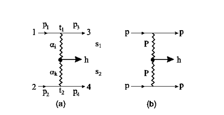
Figure 1: (a) The central production of a state h by double Reggeon-exchange. (b) The double-Pomeron exchange contributions to $pp\ \rightarrow\ p\ +\ h\ +\ p$, which dominates at high energies, where the $+$ signs are used to indicate the presence of Pomeron-induced rapidity gaps.

In figure 1 the reaction of central type

$$\begin{array}[]{l}\left\{\begin{array}[]{c}\hskip 8.5359ptH_{\ 1}\ (\ p_{\ 1}\ ;\ q.\#1\ )\vspace*{0.3cm}\\ +\ H_{\ 2}\ (\ p_{\ 2}\ ;\ q.\#2\ )\end{array}\ \right\}\ \rightarrow\left\{\begin{array}[]{c}\hskip 8.5359ptH_{\ 3}\ (\ p_{\ 3}\ ;\ q.\#3\ )\vspace*{0.3cm}\\ +\ H_{\ 4}\ (\ p_{\ 4}\ ;\ q.\#4\ )\vspace*{0.3cm}\\ +\ \left[\ h_{\ c}\ (\ p_{\ c}\ ;\ q.\#c\ )\ +\ X_{\ c}\ \right]\end{array}\right\}\end{array}$$ (1)

is represented with the following identifications

1) initial and tagged final hadron pairs inducing central production

$$\begin{array}[]{l}H_{\ 1\ ,\ 2}\ :\ \begin{array}[]{ll}\mbox{initial hadron pair}&\hskip 34.14322pt\mbox{with}\end{array}\ \left\{\begin{array}[]{cr}\mbox{momenta}&p_{\ 1\ ,\ 2}\vspace*{0.3cm}\\ \mbox{and $q.\#$}&q_{\ 1\ ,\ 2}\end{array}\right\}\vspace*{0.3cm}\\ H_{\ 3\ ,\ 4}\ :\ \begin{array}[]{ll}\begin{array}[]{l}\ \mbox{$3\ (\leftarrow\ 1)$ and $4\ (\leftarrow\ 2)$}\vspace*{0.3cm}\\ \mbox{associated hadron pair}\end{array}&\mbox{with}\end{array}\ \left\{\begin{array}[]{cr}\mbox{momenta}&p_{\ 3\ ,\ 4}\vspace*{0.3cm}\\ \mbox{and $q.\#$}&q_{\ 3\ ,\ 4}\end{array}\right\}\end{array}$$ (2)

2) centrally produced (hadronic) system $h_{\ c}$ conditioned by $h_{\ c}\ |\ X_{\ c}$

$$\begin{array}[]{l}\begin{array}[]{lll ll}h_{\ c}&:&\begin{array}[]{l}\mbox{centrally produced}\vspace*{0.3cm}\\ \mbox{system of interest}\end{array}&\mbox{with}&\left\{\begin{array}[]{cl}\mbox{momentum}&p_{\ c}\vspace*{0.3cm}\\ \mbox{mass}&M_{\ c}=\sqrt{p_{\ c}^{\ 2}}\vspace*{0.3cm}\\ \mbox{and $q.\#$}&q_{\ c}\end{array}\right\}\vspace*{0.3cm}\\ X_{\ c}&:&\mbox{{\it specified conditions}}&&\left\{\begin{array}[]{cl}\mbox{optimized to isolate}\ h_{\ c}\vspace*{0.3cm}\\ \mbox{from background}\end{array}\right\}\end{array}\end{array}$$ (3)

As is illustrated by the range of topics discussed in ref. [2] , the general issue of central production is not restricted to strong interactions limited as far as quark- and antiquark flavors are concerned to the three light ones u,d and s, denoted $QCD_{\ 3}$ hereafter.

This is our main focus here.

Rather at sufficiently high c.m. energy strong and electrweak synthesis of the central system ’$h_{\ c}$’ well includes the following processes, becoming dominantly reducible to fusion of virtual gauge boson pairs formed out of the sequence gluon (g) , photon ($\gamma$) , W , Z. We list only the combinations where $h_{\ c}\ =\ Q\overline{Q}$ $g\ g\ (\ g\ \gamma\ ,\ \gamma\gamma\ )\ \rightarrow\ Q\ \overline{Q}$ , $g\ \gamma\ \rightarrow\ Q\ \overline{Q}$ for heavy flavors $Q\ =\ c\ ,\ b\ ,\ t$ and the top quark induced hadronic production of Higgs boson(s), where $h_{\ c}\ =h^{\ JP}$ $g\ g\ \rightarrow\ t\overline{t}\ \rightarrow\ h^{\ JP}$.

i) hadronic production of (single) heavy quark-antiquark pairs, both bound and open

$$\begin{array}[]{l}h_{\ c}\ (\ QCD_{\ 6}\ )\ =\left\{\begin{array}[]{lll ll}c\overline{c}&:&J/\Psi,\chi\ ,\cdots&,&D\overline{D}\ ,\cdots\vspace*{0.3cm}\\ b\overline{b}&:&Y\ ,\chi_{\ b}\ ,\cdots&,&B\overline{B}\ ,\cdots\vspace*{0.3cm}\\ t\overline{t}&&\end{array}\right\}\vspace*{0.3cm}\\ g\ g\ \rightarrow\ Q\overline{Q}\end{array}$$ (4)

ii) hadronic production of (single) Higgs bosons $h^{\ PC}$

$$\begin{array}[]{l}h_{\ c}\ (\ QCD_{\ 6}\ ,\ {\cal{Y}}_{\ h^{\ PC}\ t\overline{t}}\ )\ =\left\{\begin{array}[]{l}h^{\ ++}\ ,\ h^{\ -+}\end{array}\right\}\vspace*{0.3cm}\\ g\ g\ \rightarrow\ t\overline{t}\ \rightarrow\ h^{\ JP}\end{array}$$ (5)

In eq. (5) ${\cal{Y}}_{\ h^{\ PC}\ t\overline{t}}$ denotes the Yukawa coupling between the Higgs boson(s) and the top quark.

The association of central production with perturbatively preconceived gauge boson fusion is not fortuitous. It goes back to seminal work on multiparticle production mainly of electrons and positrons in QED, by Landau, Lifschitz, Pomeranchuk and others. I only wish to cite a selcted subset for historical accuracy [3] .

The perturbative approach to QED governed high energy elastic scattering amplitudes for initial particle pairs $e^{-}e^{\pm}$ , $e^{-}p$ , $e^{-}\gamma$ , $\gamma p$ and $\gamma\gamma$ was pioneered by Cheng and Wu [4] . The proton can be replaced by a nucleus (A, Z), where the nuclear charge $Q\ =\ Ze$ serves to represent ’strong’ coupling, for large Z.

2 Theoretical expectations for primary gluonic binary (gb) Regge trajectories

We follow the identification of the gluonic binary states lowest in mass discussed in ref. [5].

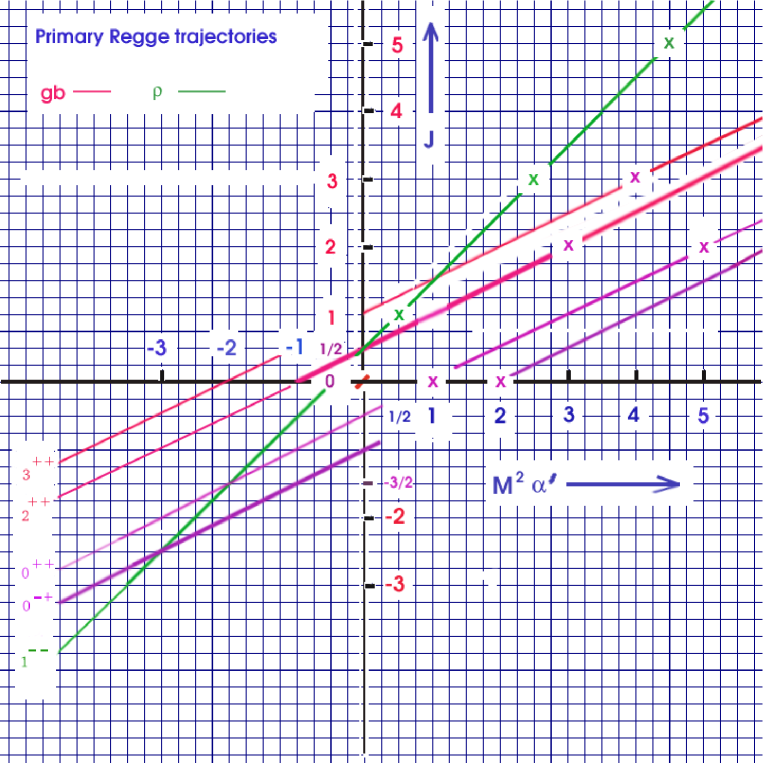
Figure 2: Primary gluonic binary (gb) Regge trajectories in comparison with the $\varrho-(q\overline{q})$ trajectory.

It shall be clear, that here we follow a combination of hypotheses and theoretical expectations. We will comment on alternatives below.

We begin with the spectrosopic classification of gluonic binaries [6], which, apart from the confined nature of binary gluons, is identical to the classification of photon binaries [7], [8].

It will prove useful to obtain a ’Richtwert’ for the inverse slope of the rho-Regge trajectory at 0 momentum transfer, since it is this quantity which sets the unit of mass square with respect to which hadronic resonances, gb and others are to be placed in the simplified harmonic and zero width- approximation.

In this objective we define the quantity $m_{\ \varrho}^{\ 2}\ (\ 0\ =\ t\ )$, which represents the $\varrho$ mass square as seen in the limit of spacelike momentum transfer $t\ \rightarrow\ 0$ through the electromagnetic form factor of charged pions $F_{\ \gamma}^{\ \pi^{\ +}}\ (\ t\ )$

$$\begin{array}[]{l}m_{\ \varrho}^{\ -2}\ (\ 0\ )\ =\ \left.d\ F_{\ \gamma}^{\ \pi^{\ +}}\ (\ t\ )\ /\ (\ dt\ )\ \right|_{\ t\ =\ 0}\ =\ \frac{1}{6}\ \left\langle\ r^{\ 2}\ \right\rangle^{\ \pi^{\ +}}_{\ \gamma}\end{array}$$ (6)

In eq. (6) $\left\langle\ r^{\ 2}\ \right\rangle^{\ \pi^{\ +}}_{\ \gamma}$ denotes the e.m. mean square charge radius of charged pions.

This quantity is presently beeing investigated by Caprini, Colangelo and
Leutwyler [9], from where I quote the preliminary result

$$\begin{array}[]{l}\left\langle\ r^{\ 2}\ \right\rangle^{\ \pi^{\ +}}_{\ \gamma}\ =\ \left\{\begin{array}[]{l}0.4332\ \pm\ 0.005\ (stat.)\ \pm\ 0.0004\ (syst.)\ \pm\ 0.0004\ (P)\vspace*{0.3cm}\\ \ \rightarrow\ 0.4332\ \pm\ 1.3\ \%\ \mbox{fm}^{\ 2}\end{array}\right.\end{array}$$ (7)

Converting to GeV units we obtain

$$\begin{array}[]{lll}m_{\ \varrho}^{\ 2}\ (\ 0\ )&=&0.5393\ \pm\ 1.3\ \%\ \mbox{GeV}^{\ 2}\vspace*{0.3cm}\\ m_{\ \varrho}^{\ 2}\ (\ 0\ )\ -\ m_{\ \pi^{0}}^{\ 2}&=&0.5211\ \pm\ 1.3\ \%\ \mbox{GeV}^{\ 2}\vspace*{0.3cm}\\ &=&\left(\ 721.9\ \pm\ 0.65\ \%\ \mbox{MeV}\ \right)^{\ 2}\end{array}$$ (8)

The quantity $m_{\ \varrho}\ (\ 0\ )$ in eq. (8) deviates substantially from the resonance parameters of the rho, whether obtained from the pole position in the complex energy plane or other parametrizations of physical cross sections. For comparison I quote a recent determination by the Kloe collaboration [10]

$$\begin{array}[]{l}m_{\ \varrho}\ =\ 775.9\ \pm\ 0.5\ \pm\ 0.3\ \mbox{MeV}\vspace*{0.3cm}\\ \Gamma_{\ \varrho}\ =\ 143.9\ \pm\ 1.3\ \pm\ 1.1\ \mbox{MeV}\end{array}$$ (9)

The relation to the inverse Regge slope parameter $(\ \alpha^{{}^{\prime}}\ )^{\ -1}$ is

$$\begin{array}[]{l}\begin{array}[]{lll}(\ \alpha^{{}^{\prime}}\ )^{\ -1}&=&2\ (\ m_{\ \varrho}^{\ 2}\ (\ 0\ )\ -\ m_{\ \pi^{0}}^{\ 2}\ )\vspace*{0.3cm}\\ &=&1.0422\ \pm\ 1.3\ \%\ \mbox{GeV}^{\ 2}\vspace*{0.3cm}\\ &=&(\ 1.0209\ \pm\ 0.65\ \%\ \mbox{GeV}\ )^{\ 2}\end{array}\end{array}$$ (10)

We remark here, that the relation in eq. (10) is not a rigorous one. We can compare with the direct $t\ >\ 0$ spectroscopic masses along the $\Lambda$ baryon trajectory, assumed unperturbed

$$\begin{array}[]{l}\frac{1}{2}\left(\ m^{2}\ (\ \Lambda^{\ 5/2+}\ )\ -m^{2}\ (\ \Lambda^{\ 1/2+}\ )\ \right)\ =\ (\ \alpha^{{}^{\prime}}_{\ \Lambda}\ )^{\ -1}=1.034\ \pm\ 0.010\ \mbox{GeV}^{\ 2}\vspace*{0.3cm}\\ \frac{1}{4}\left(\ m^{2}\ (\ \Lambda^{\ 9/2+})\ -m^{2}\ (\ \Lambda^{\ 1/2+})\ \right)\ =\ (\ \alpha^{{}^{\prime}}_{\ \Lambda}\ )^{\ -1}\ =\ 1.069\ \pm\ 0.024\ \mbox{GeV}^{\ 2}\end{array}$$ (11)

3 Quantum numbers of binary gluonic mesons

The binary gluon system is only singled out in the present discussion, because it is expected to contain gluonic meson resonances lower in mass, than ternary or more complex multi-gluonic mesons.

Let us first consider the finite dimensional (nonunitary) representations of $SL2C\ \times\ SL2C$ restricted and unrestricted to the covering group of the real Lorentz group. Details are presented in appendices A.1 and A.2 .

To this end we associate with a bosonic resonance a free, massive state or collection of spin states. Let the total spin be J. The spinor wave functions are obtained by direct products of full and chiral spin 1/2 spinors, and the four-momentumi p, neglecting here the width of the associated resonance.

$$\begin{array}[]{l}t_{\ \alpha_{1}\alpha_{2}\cdots\alpha_{N}}\ (\ p\ ;\ \left\{spin\right\}\ )\ e^{\ -ipx}\ =\ \left\langle\ \Omega\ \right|\ \phi_{\ \alpha_{1}\alpha_{2}\cdots\alpha_{N}}\ (\ x\ )\ \left|\ p\ ;\ \left\{spin\right\}\ \right\rangle\vspace*{0.3cm}\\ N\ =\ 2\ J\hskip 8.5359pt,\hskip 8.5359ptp^{\ 2}\ =\ M^{\ 2}\hskip 8.5359pt,\hskip 8.5359ptp^{\ 0}\ =\ E\ \geq\ M\vspace*{0.3cm}\\ t_{\ \alpha_{1}\alpha_{2}\cdots\alpha_{N}}\ =\ t_{\ \underline{\alpha}}\hskip 8.5359pt:\hskip 8.5359pt\begin{array}[]{l}\mbox{totally symmetric under}\vspace*{0.3cm}\\ \mbox{permutations of the indices}\end{array}\ \alpha_{1}\ \cdots\ \alpha_{N}\vspace*{0.3cm}\\ \alpha_{j}\ =\ 1,2\hskip 8.5359pt,\hskip 8.5359ptj\ =\ 1\ \cdots\ N\vspace*{0.2cm}\\ \hline\cr\vspace*{-0.2cm}\\ \widetilde{t}^{\ \dot{\gamma}_{1}\dot{\gamma}_{2}\cdots\dot{\gamma}_{N}}\ (\ p\ ;\ \left\{spin\right\}\ )\ e^{\ -ipx}\ =\ \left\langle\ \Omega\ \right|\ \psi^{\ \dot{\gamma}_{1}\dot{\gamma}_{2}\cdots\dot{\gamma}_{N}}\ (\ x\ )\ \left|\ p\ ;\ \left\{spin\right\}\ \right\rangle\vspace*{0.3cm}\\ \widetilde{t}^{\ \dot{\gamma}_{1}\dot{\gamma}_{2}\cdots\dot{\gamma}_{N}}\ =\ \widetilde{t}^{\ \underline{\dot{\gamma}}}\hskip 8.5359pt:\hskip 8.5359pt\begin{array}[]{l}\mbox{totally symmetric under}\vspace*{0.3cm}\\ \mbox{permutations of the indices}\end{array}\ \dot{\gamma}_{1}\ \cdots\ \dot{\gamma}_{N}\vspace*{0.3cm}\\ \dot{\gamma}_{j}\ =\ 1,2\hskip 8.5359pt,\hskip 8.5359ptj\ =\ 1\ \cdots\ N\end{array}$$ (12)

In eq. (12) $\left\{spin\right\}$ denotes the spin state, to be specified in a general frame of motion, and $(\ \phi_{\ \underline{\alpha}}\ ,\ \psi^{\ \underline{\dot{\gamma}}}\ )$ a pair of free fields, ( right chiral , left chiral ) , associated with the particle in question.

The transformation rules of the spinor wave functions $(\ t_{\ \underline{\alpha}}\ ,\ \widetilde{t}^{\ \underline{\dot{\gamma}}}\ )$ are

$$\begin{array}[]{l}\left\{spin\right\}\ \rightarrow\ s\hskip 8.5359pt,\hskip 8.5359pt\#\ s\ =\ N\ +\ 1\vspace*{0.3cm}\\ t_{\ \underline{\alpha}}\ (\ \Lambda p\ ;\ s\ )\ =\ S_{\ \underline{\alpha}}^{\hskip 8.5359pt\underline{\beta}}\ (\ a\ )\ t_{\ \underline{\beta}}\ (\ p\ ;\ s^{{}^{\prime}}\ )\ D_{\ s\ s^{{}^{\prime}}}\vspace*{0.3cm}\\ \widetilde{t}^{\ \underline{\dot{\gamma}}}\ (\ \Lambda p\ ;\ s\ )\ =\ \widetilde{S}^{\ \underline{\dot{\gamma}}}_{\hskip 11.38092pt\underline{\dot{\delta}}}\ (\ b\ )\ \widetilde{t}^{\ \underline{\dot{\delta}}}\ (\ p\ ;\ s^{{}^{\prime}}\ )\ D_{\ s\ s^{{}^{\prime}}}\vspace*{0.3cm}\\ D_{\ s\ s^{{}^{\prime}}}\ =\ D_{\ s\ s^{{}^{\prime}}}^{\ J}\ (\ \Lambda\ ,\ p\ )\hskip 8.5359pt;\hskip 8.5359ptb\ =\overline{a}\end{array}$$ (13)

The sought representations of the Lorentz group are obtained as symmetric products of the spin 1/2 chiral spinors. They are presented in appendix A.1 .

There is a small step from binary photon to binary gluon compounds, even though their classification with respect to quantum numbers $J^{\ PC}$ is identical.

To see this let me first discuss the $SU3_{\ c}$ gauge invariant binary gauge boson operator

$$\begin{array}[]{l}B_{\ \left[\ \mu_{1}\ \nu_{1}\ \right]\ ,\ \left[\ \mu_{2}\ \nu_{2}\ \right]}\ (\ x_{\ 1}\ ,\ x_{\ 2}\ )\ =\vspace*{0.3cm}\\ \hskip 14.22636ptF_{\ \left[\ \mu_{1}\ \nu_{1}\ \right]}\ (\ x_{\ 1}\ ;\ A\ )\ U\ (\ x_{\ 1}\ ,\ A\ ;\ x_{\ 2}\ ,\ B\ )\ F_{\ \left[\ \mu_{2}\ \nu_{2}\ \right]}\ (\ x_{\ 2}\ ;\ B\ )\vspace*{0.3cm}\\ A\ ,\ B\ ,\cdots\ =\ 1,\cdots,8\end{array}$$ (14)

Adjoint representation indices referring to the color gauge group are denoted by A , B in eq. (14). Summation over repeated such indices is implied.

$F_{\ \left[\ \mu\ \nu\ \right]}\ (\ x\ ;\ A\ )$ denote the color octet of field strengths.

The quantity $U\ (\ x\ ,\ A\ ;\ y\ ,\ B\ )$ in eq. (14) denotes the octet string operator, i. e. the path ordered exponential over a straight line path ${\cal{C}}$ from y to x.

$$\begin{array}[]{l}U\ (\ x\ ,\ A\ ;\ y\ ,\ B\ )\ =P\ \exp\ \left(\ \left.{\displaystyle{\int}}_{\ y}^{\ x}\ \right|_{\ {\cal{C}}}\ d\ z^{\ \mu}\ \frac{1}{i}\ V_{\ \mu}\ (\ z\ ,\ D\ )\ {\cal{F}}_{\ D}\ \right)_{\ A\ B}\vspace*{0.3cm}\\ \left(\ {\cal{F}}_{\ D}\ \right)_{\ AB}\ =\ i\ f_{\ A\ D\ B}\end{array}$$ (15)

In eq. (15) $f_{\ A\ D\ B}$ denotes the structure constants of $SU3_{\ c}$ and ${\cal{F}}_{\ D}$ the generators of its adjoint representation. $V_{\ \mu}\ (\ z\ ,\ D\ )$ denote the octet of field potentials.

Properties pertaining to the octet string operators, field strengths and their potentials are collected in appendix A.3 .

The extensive discussion of Stokes relations in appendix A.3 serves here to present as clear an argument as possible, why the octet string operator
$\left.U\ (\ x\ ,\ A\ ;\ y\ ,\ B\ )\ \right|_{\ {\cal{C}}}$ taken over a straight line path ${\cal{C}}$ attached to two field strength operators $F_{\ \left[\ \mu_{k}\ \nu_{k}\ \right]}\ (\ x_{\ k}\ ;\ A_{\ k}\ )\ ;\ k\ =1,2$ at the ends of the string – as displayed in eqs. (14) and (15 – form a configuration similar to an $H_{\ 2}$ molecule, representing an energetically favored gluonic meson, i.e. a hadronic resonance susceptible of identification specifically in central production.

The band structure of the $H_{\ 2}$ molecule would then translate into the possible quantum numbers of the associated binary gluonic mesons, so defined, in appropriately adapted analogy.

From a purely theoretical point of view it has to be stressed, that this remains at the present stage a hypothesis, subject to further tests, extending the existing analyses in refs. [5] and [6] as well as related and/or alternative points of view, to be substancified below.

To illustrate the molecular aspect I reproduce in figure 3 the gauge boson action density in a lattice calculcation of a nucleon [11]

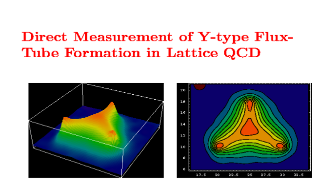
Figure 3: Gauge boson action density for a nucleon in lattice simulation of QCD.

The bilinear operator in eq. (14) satisfies Bose symmetry

$$\begin{array}[]{l}B_{\ \left[\ \mu_{1}\ \nu_{1}\ \right]\ ,\ \left[\ \mu_{2}\ \nu_{2}\ \right]}\ (\ x_{\ 1}\ ,\ x_{\ 2}\ )\ =B_{\ \left[\ \mu_{2}\ \nu_{2}\ \right]\ ,\ \left[\ \mu_{1}\ \nu_{1}\ \right]}\ (\ x_{\ 2}\ ,\ x_{\ 1}\ )\ \rightarrow\vspace*{0.3cm}\\ \widehat{C}^{\ -1}B_{\ \left[\ \mu_{1}\ \nu_{1}\ \right]\ ,\ \left[\ \mu_{2}\ \nu_{2}\ \right]}\ (\ x_{\ 1}\ ,\ x_{\ 2}\ )\ \widehat{C}\ =B_{\ \left[\ \mu_{1}\ \nu_{1}\ \right]\ ,\ \left[\ \mu_{2}\ \nu_{2}\ \right]}\ (\ x_{\ 1}\ ,\ x_{\ 2}\ )\end{array}$$ (16)

In eq. (16) $\widehat{C}$ denotes the charge conjugation operator.

We shall consider matrix elements of the form

$$\begin{array}[]{l}\left\langle\ \emptyset\ \right|\ B_{\ \left[\ \mu_{1}\ \nu_{1}\ \right]\ ,\ \left[\ \mu_{2}\ \nu_{2}\ \right]}\ (\ x_{\ 1}\ ,\ x_{\ 2}\ )\ \left|\ gb\ (\ J^{\ P\ C}\ )\ ;\ p\ ,\ \left\{spin\right\}\ \right\rangle\ \rightarrow\vspace*{0.3cm}\\ \exp^{\ -ipX}\ \widetilde{t}_{\ \underline{.}}\ (\ z\ ,\ p\ ,\ J^{\ P\ C}\ ;\ .\ )\hskip 8.5359pt\mbox{with}\vspace*{0.3cm}\\ \left|\ \emptyset\ \right\rangle\ :\ \mbox{ground state}\hskip 5.69046pt,\hskip 5.69046ptX\ =\ \frac{1}{2}\ \left(\ x_{\ 1}\ +\ x_{\ 2}\ \right)\hskip 5.69046pt,\hskip 5.69046ptz\ =\ \ \left(\ x_{\ 1}\ -\ x_{\ 2}\ \right)\vspace*{0.3cm}\\ J^{\ P\ C}\ :\ \mbox{total spin , parity , C-parity}\hskip 5.69046pt;\hskip 5.69046ptp\ :\ \mbox{c.m. four momentum}\vspace*{0.3cm}\\ \underline{.}\ :\ \mbox{spinor representation for}\ \left[\ \mu_{\ 1}\ \nu_{\ 1}\ \right]\ ,\ \left[\ \mu_{\ 2}\ \nu_{\ 2}\ \right]\vspace*{0.3cm}\\ .\ :\ \mbox{spin state}\end{array}$$ (17)

In eq. (17) $J^{\ P\ C}$ , p and $.\ =\ \left\{spin\right\}$ refer to properties of the gluonic meson in question (gb) , whereas $\underline{.}\ \leftrightarrow\ \left[\ \mu_{\ 1}\ \nu_{\ 1}\ \right]\ ,\ \left[\ \mu_{\ 2}\ \nu_{\ 2}\ \right]$ and z refer to variables initrinsic to the operator $B_{\ \left[\ \mu_{1}\ \nu_{1}\ \right]\ ,\ \left[\ \mu_{2}\ \nu_{2}\ \right]}\ (\ x_{\ 1}\ ,\ x_{\ 2}\ )$ .

The four momentum p is introduced, as if $gb\ (\ J^{\ P\ C}\ )\ ;\ p\ ,\ \left\{spin\right\}$ would correspond to a stable particle. This is at best approximately justified in the zero width approximation, which we shall not a priori assume to be valid.

Nevertheless gb-s will manifest themselves as poles in complex momentum planes, corresponding to analytic continuation of strong interaction scattering amplitudes. The latter refer to stable particles, like pions, kaons and baryons, in the limit where both electromagnetic and weak interactions are neglected.

Hence, ignoring the above complication for the time beeing, the mass of $gb\ (\ J^{\ P\ C}\ )$ is defined through p

$$\begin{array}[]{l}m^{\ 2}\ =\ p_{\ \mu}\ p^{\ \mu}\hskip 5.69046pt;\hskip 5.69046ptE_{\ p}\ =\ \sqrt{\ p^{\ 2}\ +\ m^{\ 2}}\vspace*{0.3cm}\\ m\ =\ m\ \left(\ gb\ (\ J^{\ P\ C}\ )\ \right)\end{array}$$ (18)

As a consequence of eq. (16) we have for binary gluonic mesons $C\ =\ +$ throughout.

$$\begin{array}[]{l}gb\ (\ J^{\ P\ C}\ )\ \rightarrow gb\ (\ J^{\ P\ +}\ )\end{array}$$ (19)

The relativistic spin $\underline{.}$ , processed as outlined in appendix A.1 , combines the same way as in the nonrelativistic case to a total spin $S_{\ 12}$

$$\begin{array}[]{l}S_{\ 12}\ =\ S_{\ 12}^{\ +}\ +\ S_{\ 12}^{\ -}\vspace*{0.3cm}\\ \left(\ S_{\ 12}^{\ +}\ =\ 0\ ,\ 2\hskip 5.69046pt\leftrightarrow\hskip 5.69046ptP\ =\ +\ \right)\hskip 5.69046pt;\hskip 5.69046pt\left(\ S_{\ 12}^{\ -}\ =\ 1\hskip 5.69046pt\leftrightarrow\hskip 5.69046ptP\ =\ -\ \right)\end{array}$$ (20)

The total spin states $S_{\ 12}$ in eq. (20) are subject to transversity conditions, to which we will turn below. But independtly thereof the spectrum of $gb\ (\ J^{\ P\ +}\ )$ at this stage splits into three

$$\begin{array}[]{l}gb\ (\ J^{\ P\ +}\ )\ \begin{array}[]{lll ll}\nearrow&gb\ (\ J^{\ +\ +}\ )&,&S_{\ 12}^{\ +}\ =\ 2&\hskip 8.5359pt:\hskip 8.5359ptII^{\ +}\vspace*{0.3cm}\\ \rightarrow&gb\ (\ J^{\ +\ +}\ )&,&S_{\ 12}^{\ +}\ =\ 0&\hskip 8.5359pt:\hskip 8.5359ptI^{\ +}\vspace*{0.3cm}\\ \searrow&gb\ (\ J^{\ -\ +}\ )&,&S_{\ 12}^{\ -}\ =\ 1&\hskip 8.5359pt:\hskip 8.5359ptI^{\ -}\end{array}\end{array}$$ (21)

The three spectral types shall be denoted as in eq. (21) : $II^{\ +}$ , $I^{\ +}$ and $I^{\ -}$ , where the superfix stands for parity.

To clarify the spin structure we discuss the spectral classes $I^{\ \pm}$ first. To this end we label the amplitudes $\widetilde{t}_{\ \underline{.}}\ (\ z\ ,\ p\ ,\ J^{\ P\ C}\ ;\ .\ )$ in eq. (17)

$$\begin{array}[]{l}\widetilde{t}_{\ \underline{.}}\ (\ z\ ,\ p\ ,\ J^{\ P\ +}\ ;\ .\ )\ \rightarrow\ \widetilde{t}_{\ \underline{.}\ ;\ S_{\ 12}^{\ \pm}}\ (\ z\ ,\ p\ ,\ J^{\ \pm\ +}\ ;\ .\ )\vspace*{0.3cm}\\ \hline\cr\vspace*{-0.2cm}\\ \widetilde{t}_{\ \underline{.}\ ;\ S_{\ 12}^{\ \pm}}\ (\ z\ ,\ p\ ,\ J^{\ \pm\ +}\ ;\ .\ )\begin{array}[]{ll}\nearrow&\widetilde{t}_{\ \underline{.}\ ;\ II^{\ +}}\ (\ z\ ,\ p\ ,\ J^{\ +\ +}\ ;\ .\ )\vspace*{0.3cm}\\ \rightarrow&\widetilde{t}_{\ \underline{.}\ ,\ I^{\ +}}\ (\ z\ ,\ p\ ,\ J^{\ +\ +}\ ;\ .\ )\vspace*{0.3cm}\\ \searrow&\widetilde{t}_{\ \underline{.}\ ;\ I^{\ -}}\ (\ z\ ,\ p\ ,\ J^{\ -\ +}\ ;\ .\ )\end{array}\vspace*{0.3cm}\\ \underline{.}\ ;S_{\ 12}^{\ \pm}\ \rightarrow\ \underline{.}\ \rightarrow\ \left[\ \mu_{\ 1}\ \nu_{\ 1}\ \right]\ ,\ \left[\ \mu_{\ 2}\ \nu_{\ 2}\ \right]\end{array}$$ (22)

The two spectral classes $I^{\ \pm}$ exhibit the relativistic factorization patterns

$$\begin{array}[]{l}\widetilde{t}_{\ \underline{.}\ ;\ I^{\ \pm}}\ (\ z\ ,\ p\ ,\ J^{\ \pm\ +}\ ;\ .\ )\ =\ \left(\begin{array}[]{l}\ \left(\ K^{\ \pm}\ \right)_{\ \ \left[\ \mu_{\ 1}\ \nu_{\ 1}\ \right]\ \left[\ \mu_{\ 2}\ \nu_{\ 2}\ \right]}\ \times\vspace*{0.3cm}\\ \hskip 19.91684pt\times\ \widetilde{t}_{\ I^{\ \pm}}\ (\ z\ ,\ p\ ,\ J^{\ \pm\ +}\ ;\ .\ )\end{array}\ \right)\vspace*{0.5cm}\\ \ \left(\ K^{\ +}\ \right)_{\ \ \left[\ \mu_{\ 1}\ \nu_{\ 1}\ \right]\ \left[\ \mu_{\ 2}\ \nu_{\ 2}\ \right]}\ =\ g_{\ \mu_{\ 1}\ \mu_{\ 2}}\ g_{\ \nu_{\ 1}\ \nu_{\ 2}}\ -\ g_{\ \mu_{\ 1}\ \nu_{\ 2}}\ g_{\ \mu_{\ 2}\ \nu_{\ 1}}\vspace*{0.5cm}\\ \ \left(\ K^{\ -}\ \right)_{\ \ \left[\ \mu_{\ 1}\ \nu_{\ 1}\ \right]\ \left[\ \mu_{\ 2}\ \nu_{\ 2}\ \right]}\ =\ \varepsilon_{\ \mu_{\ 1}\ \mu_{\ 2}\ \nu_{\ 1}\ \nu_{\ 2}}\end{array}$$ (23)

In eq. (23) $K^{\ \pm}$ denote the two Lorentz invariant tensors with parity $\pm$ respectively and $g_{\ \mu\nu}$ the Lorentz metric tensor.

The tensors $K^{\ \pm}$ form projection operations on the octet string operators

$$B_{\ \left[\ \mu_{1}\ \nu_{1}\ \right]\ ,\ \left[\ \mu_{2}\ \nu_{2}\ \right]}\ (\ x_{\ 1}\ ,\ x_{\ 2}\ )$$

introduced in eq. (14) , described in appendix A.4 .

The projections yield

$$\begin{array}[]{l}B_{\ \left[\ \mu_{1}\ \nu_{1}\ \right]\ ,\ \left[\ \mu_{2}\ \nu_{2}\ \right]}\ (\ x_{\ 1}\ ,\ x_{\ 2}\ )\ =\left(\begin{array}[]{r}\left(\ K^{\ +}\ \right)_{\ \ \left[\ \mu_{\ 1}\ \nu_{\ 1}\ \right]\ \left[\ \mu_{\ 2}\ \nu_{\ 2}\ \right]}\ B^{\ (+)}\vspace*{0.3cm}\\ +\ \left(\ K^{\ -}\ \right)_{\ \ \left[\ \mu_{\ 1}\ \nu_{\ 1}\ \right]\ \left[\ \mu_{\ 2}\ \nu_{\ 2}\ \right]}\ B^{\ (-)}\vspace*{0.3cm}\\ +\ B^{\ {}^{\prime}}_{\ \left[\ \mu_{1}\ \nu_{1}\ \right]\ ,\ \ \left[\ \mu_{2}\ \nu_{2}\ \right]}\end{array}\right)\vspace*{0.2cm}\end{array}$$ (24)

where the quantities $B^{\ (\pm)}$ are derived in appendix A.4 . They are of the form given in eq. (160) reproduced below

$$\begin{array}[]{l}B^{\ (+)}\ (\ x_{\ 1}\ ,\ x_{\ 2}\ )\ =\vspace*{0.3cm}\\ \hskip 17.07182pt=\ \frac{1}{12}\ F_{\ \left[\ \alpha\ \beta\ \right]}\ (\ x_{\ 1}\ ;\ A\ )\ U\ (\ x_{\ 1}\ ,\ A\ ;\ x_{\ 2}\ ,\ B\ )\ F^{\ \left[\ \alpha\ \beta\ \right]}\ (\ x_{\ 2}\ ;\ B\ )\vspace*{0.3cm}\\ \hline\cr\vspace*{-0.2cm}\\ B^{\ (-)}\ (\ x_{\ 1}\ ,\ x_{\ 2}\ )\ =\vspace*{0.3cm}\\ \hskip 17.07182pt=\ -\ \frac{1}{12}\ F_{\ \left[\ \alpha\ \beta\ \right]}\ (\ x_{\ 1}\ ;\ A\ )\ U\ (\ x_{\ 1}\ ,\ A\ ;\ x_{\ 2}\ ,\ B\ )\ \widetilde{F}^{\ \left[\ \alpha\ \beta\ \right]}\ (\ x_{\ 2}\ ;\ B\ )\vspace*{0.3cm}\\ \hskip 17.07182pt=\ -\ \frac{1}{12}\ \widetilde{F}_{\ \left[\ \alpha\ \beta\ \right]}\ (\ x_{\ 1}\ ;\ A\ )\ U\ (\ x_{\ 1}\ ,\ A\ ;\ x_{\ 2}\ ,\ B\ )\ F^{\ \left[\ \alpha\ \beta\ \right]}\ (\ x_{\ 2}\ ;\ B\ )\vspace*{0.3cm}\\ \hline\cr\vspace*{-0.2cm}\\ \widetilde{F}_{\ \left[\ \alpha\ \beta\ \right]}\ (\ x_{\ 2}\ ;\ B\ )\ =\ \frac{1}{2}\ \varepsilon_{\ \alpha\ \beta\ \gamma\ \delta}\ F^{\ \left[\ \gamma\ \delta\ \right]}\ (\ x_{\ 2}\ ;\ B\ )\vspace*{0.3cm}\\ \mbox{and}\hskip 8.5359pt(\ x_{\ 2}\ ;\ B\ )\ \leftrightarrow\ (\ x_{\ 1}\ ;\ A\ )\end{array}$$ (25)

Returning to the (spin-) reduced amplitudes $\widetilde{t}_{\ I^{\ \pm}}\ (\ z\ ,\ p\ ,\ J^{\ \pm\ +}\ ;\ .\ )$ introduced in eq. (23) we obtain using the notation of eq. (17)

$$\begin{array}[]{l}\left\langle\ \emptyset\ \right|\ B^{\ (\pm)}\ (\ x_{\ 1}\ ,\ x_{\ 2}\ )\ \left|\ gb_{\ I^{\ \pm}}\ (\ J^{\ \pm\ +}\ )\ ;\ p\ ,\ \left\{spin\right\}\ \right\rangle\ =\vspace*{0.3cm}\\ \hskip 8.5359pt=\ \exp^{\ -ipX}\ \widetilde{t}_{\ I^{\ \pm}}\ (\ z\ ,\ p\ ,\ J^{\ \pm\ +}\ ;\ .\ )\end{array}$$ (26)

with $B^{\ (\pm)}$ given in eq. (25) . In eq. (26) the suffix $I^{\ \pm}$ of the states $gb_{\ I^{\ \pm}}$ indicates, that these are restricted to the spectral types denoted $I^{\ \pm}$ in eq. (21) .

In the local limit of $z\ \rightarrow\ 0$ , i.e. shrinking the extension of the adjoint string to zero length, we recognize in $B^{\ (\pm)}$ two local operators shaping the dynamics of QCD. We ignore here for clarity all short distance singularities, in this limit.

$$\begin{array}[]{l}z\ \rightarrow\ 0\hskip 8.5359pt:\hskip 8.5359pt\begin{array}[]{l lr}B^{\ (+)}&\rightarrow&\frac{1}{12}\ F_{\ \left[\ \mu\ \nu\ \right]}\ (\ X\ ;\ A\ )\ F^{\ \left[\ \mu\ \nu\ \right]}\ (\ X\ ;\ A\ )\vspace*{0.3cm}\\ B^{\ (-)}&\rightarrow&-\ \frac{1}{12}\ F_{\ \left[\ \mu\ \nu\ \right]}\ (\ X\ ;\ A\ )\ \widetilde{F}^{\ \left[\ \mu\ \nu\ \right]}\ (\ X\ ;\ A\ )\end{array}\ \rightarrow\vspace*{0.4cm}\\ \hline\cr\vspace*{-0.3cm}\\ \begin{array}[]{l|l}\begin{array}[]{rll}3\ \left.B^{\ (+)}\ \right|_{\ 0}&=&{\cal{L}}^{\ (+)}\ (\ X\ )\vspace*{0.3cm}\\ -\ 3\ \left.B^{\ (-)}\ \right|_{\ 0}&=&{\cal{L}}^{\ (-)}\ (\ X\ )\end{array}&\begin{array}[]{rll}{\cal{L}}^{\ (+)}\ (\ X\ )&=&g^{\ 2}\ s\ (\ X\ )\vspace*{0.3cm}\\ {\cal{L}}^{\ (-)}\ (\ X\ )&=&8\ \pi^{\ 2}\ ch_{\ 2}\ (\ X\ )\end{array}\end{array}\vspace*{0.4cm}\\ \hline\cr\vspace*{-0.3cm}\\ \begin{array}[]{rll}{\cal{L}}^{\ (+)}\ (\ X\ )&=&\ \frac{1}{4}\ F_{\ \left[\ \mu\ \nu\ \right]}\ (\ X\ ;\ A\ )\ F^{\ \left[\ \mu\ \nu\ \right]}\ (\ X\ ;\ A\ )\vspace*{0.3cm}\\ {\cal{L}}^{\ (-)}\ (\ X\ )&=&\frac{1}{4}\ F_{\ \left[\ \mu\ \nu\ \right]}\ (\ X\ ;\ A\ )\ \widetilde{F}^{\ \left[\ \mu\ \nu\ \right]}\ (\ X\ ;\ A\ )\end{array}\end{array}$$ (27)

In eq. (27) $s$ denotes the action density pertaining to gauge bosons and g the (strong) coupling constant, while $ch_{\ 2}$ represents the density of the second Chern character.

We return to the wave functions $\widetilde{t}_{\ I^{\ \pm}}\ (\ z\ ,\ p\ ,\ J^{\ \pm\ +}\ ;\ .\ )$ defined in eqs. (23) and (26) pertaining to the gb spectral types $I^{\ \pm}$ in eq. (26) . As a consequence of eq. (16) they satisfy the Bose symmetry relation

$$\begin{array}[]{l}\widetilde{t}_{\ I^{\ \pm}}\ (\ z\ ,\ p\ ,\ J^{\ \pm\ +}\ ;\ .\ )\ =\widetilde{t}_{\ I^{\ \pm}}\ (\ -\ z\ ,\ p\ ,\ J^{\ \pm\ +}\ ;\ .\ )\end{array}$$ (28)

We meet a problem of interpretation of the bilinear wave functions $\widetilde{t}_{\ I^{\ \pm}}$ and the symmetry in eq. (28) , known (also) from the study of $q\overline{q}$ and 3 q composite systems [12].

This is recognized, decomposing the Lorentz four vector z into parallel and transverse components relative to the c.m. momentum p

$$\begin{array}[]{l}z\ =\ z_{\ p}\ +\ \eta\ p\ /\ m^{\ 2}\hskip 8.5359pt;\hskip 8.5359pt\eta\ =\ z\ p\hskip 8.5359pt\rightarrow\hskip 8.5359ptz_{\ p}\ p\ =\ 0\end{array}$$ (29)

In the c.m. system the scalar product $\eta$ in eq. (29) becomes relative time, which is not a genuine degree of freedom of the dynamical system in question.

$$\begin{array}[]{l}\mbox{c.m. :}\hskip 8.5359ptp\ \rightarrow\ p_{\ c.m.}\ (\ m\ ,\ \vec{0}\ )\vspace*{0.3cm}\\ \eta\ \rightarrow\ m\ z_{\ 0}\ =\ m\ t_{\ rel}\end{array}$$ (30)

Let me illustrate what is addressed here, considering the decay $\varrho^{\ 0}\ \rightarrow\ 2\ \pi$ .

First we shall assume pions to be absolutely stable. Then the decay

$$\varrho^{\ 0}\ \rightarrow\ 2\ \pi^{\ 0}$$

is forbidden by Bose symmetry. Next we take into account, that $\pi^{\ 0}$ s decay (mainly) into two photons, over the width of $\pi^{\ 0}$. The latter is according to the PDG [13]

$$\begin{array}[]{l}\tau_{\ \pi^{\ 0}}\ =\ \left(\ 8.4\ \pm\ 0.6\ \right)\ 10^{\ -17}\ \mbox{sec}\hskip 8.5359pt\leftrightarrow\hskip 8.5359pt\Gamma_{\ \pi^{\ 0}}\ =\ \left(\ 7.84\ \pm\ 0.53\ \right)\ \mbox{eV}\end{array}$$ (31)

To be specific we consider the reaction

$$\begin{array}[]{l}e^{+}\ e^{-}\ \rightarrow\ \varrho^{\ 0}\ \rightarrow\ 4\ \gamma\end{array}$$ (32)

and ask the question, whether it can proceed, when the two pairs of photons, $\gamma_{\ 1}\ \gamma_{\ 2}$ and $\gamma_{\ 3}\ \gamma_{\ 4}$ say, form each a $\pi^{\ 0}$ , with invariant masses $m_{\ 12}$ and $m_{\ 34}$ differing by a well defined fraction of $\Gamma_{\ \pi^{\ 0}}$

$$\begin{array}[]{l}f_{+}\ \Gamma_{\ \pi^{\ 0}}\ \geq\left|\ m_{\ 12}\ -\ m_{\ 34}\ \right|\ \geq\ f_{-}\ \Gamma_{\ \pi^{\ 0}}\vspace*{0.3cm}\\ \mbox{with}\hskip 11.38092pt\ f_{+}\ =\ 1\hskip 8.5359pt,\hskip 8.5359pt\ f_{-}\ =\ 0.1\hskip 11.38092pt\mbox{say}\end{array}$$ (33)

The answer relevant here is, that there is a multitude of equivalent irreducible wave functions out of the family defined in eqs. (23) and (26)

$$\begin{array}[]{l}\widetilde{t}_{\ I^{\ \pm}}\ (\ z\ ,\ p\ ,\ J^{\ \pm\ +}\ ;\ .\ )\ =\widetilde{t}_{\ I^{\ \pm}}\ (\ z_{\ p}\ ,\ p\ ,\ \eta\ ,\ J^{\ \pm\ +}\ ;\ .\ )\end{array}$$ (34)

distinguished by the parameter $\eta$ as defined in eqs. (29) and (30).

Thus we choose the representative with $\eta\ =\ 0$

$$\begin{array}[]{l}t_{\ I^{\ \pm}}\ (\ z_{\ p}\ ,\ p\ ,\ J^{\ \pm\ +}\ ;\ .\ )\ =\widetilde{t}_{\ I^{\ \pm}}\ (\ z_{\ p}\ ,\ p\ ,\ \eta\ =\ 0\ ,\ J^{\ \pm\ +}\ ;\ .\ )\end{array}$$ (35)

The above procedure illustrates the difference between decay amplitudes of resonances into two photons and their selection rules, derived in refs. [7] and [8], and the wave functions of binary gluonic mesons.

The irreducible wave functions $t_{\ I^{\ \pm}}$ can readily be discussed in the rest system of the momentum p, where

$$\begin{array}[]{l}\mbox{c.m. :}\hskip 8.5359pt\left(\ \eta\ =\ 0\ ,\ z_{\ p}\ \right)\ \rightarrow\ z_{\ p}\ =\ \left(\ 0\ ,\ \vec{z}\ \right)\ \rightarrow\ \vec{z}\vspace*{0.3cm}\\ t_{\ I^{\ \pm}}\ (\ z_{\ p}\ ,\ p\ ,\ J^{\ \pm\ +}\ ;\ .\ )\ \rightarrow t_{\ I^{\ \pm}}\ (\ \vec{z}\ ,\ J^{\ \pm\ +}\ ;\ .\ )\end{array}$$ (36)

The procedure outlined above implies, that the octet string bilinear operators

$$\begin{array}[]{l}B_{\ \left[\ \mu_{1}\ \nu_{1}\ \right]\ ,\ \left[\ \mu_{2}\ \nu_{2}\ \right]}\ (\ x_{\ 1}\ ,\ x_{\ 2}\ )\end{array}$$ (37)

defined in eq. (14) are to be evaluated for spacelike relative positions
$z\ =\ x_{\ 1}\ -\ x_{\ 2}$ only.

Now eq. (28) takes the form

$$\begin{array}[]{l}t_{\ I^{\ \pm}}\ (\ \vec{z}\ ,\ J^{\ \pm\ +}\ ;\ .\ )\ =\ t_{\ I^{\ \pm}}\ (\ -\ \vec{z}\ ,\ J^{\ \pm\ +}\ ;\ .\ )\end{array}$$ (38)

The consequence for the angular momentum composition of the spectral types $I^{\ \pm}$ is indeed identical to the situation of decay into two photons [7] , [8]

$$\begin{array}[]{l}t_{\ I^{\ \pm}}\ (\ \vec{z}\ ,\ J^{\ \pm\ +}\ ;\ .\ )\ \rightarrow\ t_{\ I^{\ \pm}}\ (\ \vec{z}\ ,\ J^{\ \pm\ +}\ ;\ M\ )\vspace*{0.3cm}\\ t_{\ I^{\ \pm}}\ (\ \vec{z}\ ,\ J^{\ \pm\ +}\ ;\ M\ )\ =\ R^{\ J}_{\ I^{\ \pm}}\ (\ r\ )\ Y^{\ J}_{\ M}\ (\ \vec{e}\ )\hskip 8.5359pt;\hskip 8.5359ptJ\ =\ \mbox{even}\vspace*{0.3cm}\\ r\ =\ \left|\ \vec{z}\ \right|\hskip 8.5359pt,\hskip 8.5359pt\vec{e}\ =\ \vec{z}\ /\ r\vspace*{0.4cm}\\ \hline\cr\vspace*{-0.3cm}\\ \begin{array}[]{lll}I^{\ +}&:&J^{\ P\ C}\ =\ 0^{\ ++}\ ,\ 2^{\ ++}\ ,\ 4^{\ ++}\ \cdots\vspace*{0.3cm}\\ I^{\ -}&:&J^{\ P\ C}\ =\ 0^{\ -+}\ ,\ 2^{\ -+}\ ,\ 4^{\ -+}\ \cdots\end{array}\end{array}$$ (39)

In eq. (39) $Y^{\ J}_{\ M}$ denote the orbital spherical harmonics with angular momentum J , while $\left\{\ R^{\ J}_{\ I^{\ \pm}}\ \right\}$ stand for a family of radial wave functions. Neither nature nor extension of this family, nor its ordering in mass can be deduced from the spectral type.

For the sake of absolute clarity let me emphasize that the family of wave functions (of all types pertinent to binary gluonic mesons) can be empty, since no first principle proof to the contrary exists.

Quantum numbers of binary gluonic mesons continued

The $II^{\ +}$ spectral type

We turn to the remaining spectral type denoted $II^{\ +}$ in eq. (21) .

The properties of this spectral series, represented by the quantities
$B^{\ {}^{\prime}}_{\ \left[\ \mu_{1}\ \nu_{1}\ \right]\ ,\ \ \left[\ \mu_{2}\ \nu_{2}\ \right]}$ defined in eq. (24) are derived in appendix A.5 .

As shown there the wave functions of the gb spectral type $II^{\ +}$ are uniquely associated with the classical energy momentum bilinear pertaining to gauge bosons.

We retain here the characteristic composition of the wave function associated bilinears $B^{\ {}^{\prime}}$ in eqs. (218) and (219) in the summary remarks of appendix A.5:

$$\begin{array}[]{l}B_{\ \left[\ \mu_{1}\ \nu_{1}\ \right]\ ,\ \left[\ \mu_{2}\ \nu_{2}\ \right]}\ =\ \left\{\begin{array}[]{c}\ \frac{1}{2}\left(\begin{array}[]{l}g_{\ \mu_{\ 1}\ \mu_{\ 2}}\ \varrho_{\ \nu_{\ 1}\ \nu_{\ 2}}-\ g_{\ \nu_{\ 1}\ \mu_{\ 2}}\ \varrho_{\ \mu_{\ 1}\ \nu_{\ 2}}\vspace*{0.3cm}\\ -\ g_{\ \mu_{\ 1}\ \nu_{\ 2}}\ \varrho_{\ \nu_{\ 1}\ \mu_{\ 2}}\ +\ g_{\ \nu_{\ 1}\ \nu_{\ 2}}\ \varrho_{\ \mu_{\ 1}\ \mu_{\ 2}}\end{array}\right)\vspace*{0.3cm}\\ +\ K^{\ +}_{\ \left[\ \mu_{1}\ \nu_{1}\ \right]\ \left[\ \mu_{2}\ \nu_{2}\ \right]}\ B^{\ (+)}\vspace*{0.3cm}\\ +\ K^{\ -}_{\ \left[\ \mu_{1}\ \nu_{1}\ \right]\ \left[\ \mu_{2}\ \nu_{2}\ \right]}\ B^{\ (-)}\vspace*{0.3cm}\\ \end{array}\right\}\vspace*{0.4cm}\\ \hline\cr\vspace*{-0.3cm}\\ \mbox{with :}\ g^{\ \mu_{\ 1}\ \mu_{\ 2}}\ B_{\ \left[\ \mu_{1}\ \nu_{1}\ \right]\ ,\ \left[\ \mu_{2}\ \nu_{2}\ \right]}\ =\ R_{\ \nu_{\ 1}\ \nu_{\ 2}}\vspace*{0.5cm}\\ -\ \varrho^{\ \mu\ \nu}\ =\ -\ R^{\ \mu\ \nu}\ +\ \frac{1}{4}\ g^{\ \mu\ \nu}\ R\ =\ \vartheta_{\ cl}^{\ \mu\ \nu}\vspace*{0.5cm}\\ R\ =\ g^{\ \nu_{\ 1}\ \nu_{\ 2}}\ R_{\ \nu_{\ 1}\ \nu_{\ 2}}\ =\ 12\ B^{\ (+)}\end{array}$$ (40)

The bilinears $B^{\ {}^{\prime}}$ are thus given by

$$\begin{array}[]{l}B^{\ {}^{\prime}}_{\ \left[\ \mu_{1}\ \nu_{1}\ \right]\ ,\ \ \left[\ \mu_{2}\ \nu_{2}\ \right]}\ =\ \frac{1}{2}\left(\begin{array}[]{l}g_{\ \mu_{\ 1}\ \mu_{\ 2}}\ \varrho_{\ \nu_{\ 1}\ \nu_{\ 2}}-\ g_{\ \nu_{\ 1}\ \mu_{\ 2}}\ \varrho_{\ \mu_{\ 1}\ \nu_{\ 2}}\vspace*{0.3cm}\\ -\ g_{\ \mu_{\ 1}\ \nu_{\ 2}}\ \varrho_{\ \nu_{\ 1}\ \mu_{\ 2}}\ +\ g_{\ \nu_{\ 1}\ \nu_{\ 2}}\ \varrho_{\ \mu_{\ 1}\ \mu_{\ 2}}\end{array}\right)\vspace*{0.3cm}\\ B^{\ {}^{\prime}}\ \leftrightarrow\ \left\{\ II^{\ +}\ \right\}\ \longleftrightarrow\ \vartheta_{\ cl}^{\ \mu\ \nu}\end{array}$$ (41)

The three spectral types are given in eq. (42) below, completing the types $I^{\ \pm}$ in eq. (39)

$$\begin{array}[]{l}t_{\ I^{\ \pm}}\ (\ \vec{z}\ ,\ J^{\ \pm\ +}\ ;\ .\ )\ \rightarrow\ t_{\ I^{\ \pm}}\ (\ \vec{z}\ ,\ J^{\ \pm\ +}\ ;\ M\ )\vspace*{0.3cm}\\ t_{\ I^{\ \pm}}\ (\ \vec{z}\ ,\ J^{\ \pm\ +}\ ;\ M\ )\ =\ R^{\ J}_{\ I^{\ \pm}}\ (\ r\ )\ Y^{\ J}_{\ M}\ (\ \vec{e}\ )\hskip 8.5359pt;\hskip 8.5359ptJ\ =\ \mbox{even}\vspace*{0.3cm}\\ r\ =\ \left|\ \vec{z}\ \right|\hskip 8.5359pt,\hskip 8.5359pt\vec{e}\ =\ \vec{z}\ /\ r\vspace*{0.4cm}\\ \hline\cr\vspace*{-0.3cm}\\ \begin{array}[]{lll}I^{\ +}&:&J^{\ P\ C}\ =\ 0^{\ ++}\ ,\ 2^{\ ++}\ ,\ 4^{\ ++}\ \cdots\vspace*{0.3cm}\\ I^{\ -}&:&J^{\ P\ C}\ =\ 0^{\ -+}\ ,\ 2^{\ -+}\ ,\ 4^{\ -+}\ \cdots\end{array}\vspace*{0.4cm}\\ \hline\cr\hline\cr\vspace*{-0.3cm}\\ t_{\ II^{\ +}}\ (\ \vec{z}\ ,\ J^{\ \pm\ +}\ ;\ .\ )\ \rightarrow\ t_{\ II^{\ +}}\ (\ \vec{z}\ ,\ J^{\ II\ +}\ ;\ M\ ,\ \vec{E}_{\ \pm}\ )\vspace*{0.4cm}\\ t_{\ II^{\ +}}\ (\ \vec{z}\ ,\ J^{\ II\ +}\ ;\ M\ ,\ \vec{E}_{\ \pm}\ )\ =\vspace*{0.4cm}\\ \hskip 11.38092pt=\ R^{\ J}_{\ II^{\ +}}\ (\ r\ ,\ \vec{E}_{\ \pm}\ )\ D^{\ J}_{\ M\ \pm 2}\ (\ \vec{e}\ ,\ \vec{E}_{\ \pm}\ )\vspace*{0.4cm}\\ \begin{array}[]{lll}II^{\ +}&:&J^{\ P\ C}\ =\ 2^{\ ++}\ ,\ 3^{\ ++}\ ,\ 4^{\ ++}\ ,\ 5^{\ ++}\ \cdots\end{array}\vspace*{0.3cm}\\ \hline\cr\end{array}$$ (42)

In eq. (42) the chromoelectric field strengths $\vec{E}_{\ \pm}$ are retained in the arguments of the wave functions.

The functions $D^{\ J}_{\ M\ \sigma}\ (\ \vec{e}\ ,\ \vec{E}_{\ \pm}\ )$ , with $\sigma\ =\ \pm 2$ , denote the eigenfunctions of a (symmetric) top, with the full orientation involving three Euler angles provided by the correlation between the two chromoelectric field strengths $\vec{E}_{\ \pm}$ of the adjoint string, discussed in appendix A.5 .

Let us end here the theoretical discussion of binary gluonic modes associated with the octet gauge boson string. Theoretical expectations of spectral characteristics of states representing the spectral types $I^{\ \pm}$ and $II^{\ +}$ shall be addressed in the next section.

4 Spectral patterns of gb - facts and fancy

a) Lattice QCD calculations

The most promising and widely accepted framework to derive spectral patterns of hadrons, including gluonic mesons, is lattice gauge theory and therein the restriction to gauge boson degrees of freedom only. I shall quote several papers instead of a review : [14] , [15] , [16] and [17] .

I shall discuss the above papers one by one. In ref. [14] a careful and dedicated study is devoted to the determination of the mass of $gb\ (\ 0^{\ ++}\ )$ , the lowest lying gluonic meson in pure Yang-Mills theory based on $SU3_{\ c}$ , and also $gb\ (\ 2^{++}\ )$ , with the results

$$\begin{array}[]{l}m\ \left(\ gb\ (\ 0^{++}\ )\ \right)\ =\ 1627\ \pm\ 83\ \mbox{MeV}\ \rightarrow\ m^{\ 2}\ =\ 2.65\ \pm\ 0.27\ \mbox{GeV}^{\ 2}\vspace*{0.3cm}\\ m\ \left(\ gb\ (\ 2^{++}\ )\ \right)\ =\ 2354\ \pm\ 95\ \mbox{MeV}\ \rightarrow\ m^{\ 2}\ =\ 5.54\ \pm\ 0.6\ \mbox{GeV}^{\ 2}\end{array}$$ (43)

The main result refers to $gb\ (\ 0^{\ ++}\ )$ and is in very good agreement with all lattice gauge theory calculations, concerning the same state.

I compare the above results with the assignment made here in figure 2

$$\begin{array}[]{l}m^{\ 2}\ \left(\ gb\ (\ 0^{++}\ )\ \right)\ =\ 1.04\ \mbox{GeV}^{\ 2}\vspace*{0.3cm}\\ m^{\ 2}\ \left(\ gb\ (\ 2^{++}\ )\ \right)\ =\ 3.13\ \mbox{GeV}^{\ 2}\end{array}$$ (44)

While it is difficult to associate an error with the tentative pattern represented in figure 2 and eq. (44) , to which I will return below, the essentially smaller mass square scale, by factors of $\sim\ 2.5$ and $\sim\ 1.8$ for $gb\ (\ 0^{\ ++}\ )$ and $gb\ (\ 2^{\ ++}\ )$ respectively, is indeed a basic controversy, seemingly disproving the mass square range considered in eq. (44) .

In ref. [15] an attempt is made to align gb resonances on the Pomeron trajectory, as done here in figure 2, but with very different assignments : the slope of the Pomeron trajectory is assumed to be

$$\begin{array}[]{l}\cite[cite]{[\@@bibref{}{Teper}{}{}]}\ :\ \alpha^{\ {}^{\prime}}_{\ P}\ =\ \ \alpha^{\ {}^{\prime}}_{\ g\ b}\ \sim\ 0.22\ \pm\ 0.4\ \mbox{GeV}^{\ -2}\vspace*{0.3cm}\\ \mbox{here}\ :\ \ \alpha^{\ {}^{\prime}}_{\ g\ b}\ =\ \frac{1}{2}\ \alpha^{\ {}^{\prime}}\ =\ 0.5211\ \pm\ 1.3\ \%\ \mbox{GeV}^{\ -2}\end{array}$$ (45)

Again a factor of two opens up, with respect to the value of $\alpha^{\ {}^{\prime}}_{\ gb}$, between ref. [15] and our present discussion, where indeed the relation $\alpha^{\ {}^{\prime}}_{\ gb}\ =\ \frac{1}{2}\ \alpha^{\ {}^{\prime}}$ , also discussed below, can be in doubt.

As a consequence of the calculations in ref. [15] the deduced mass square value for $gb\ (\ 2^{\ ++}\ )$ , which is supposed to lye on the Pomeron trajectory, becomes

$$\begin{array}[]{l}\cite[cite]{[\@@bibref{}{Teper}{}{}]}\ :\ m^{\ 2}\ \left(\ gb\ (\ 2^{++}\ )\ \right)\ =\ 4.4\ \pm\ 1.2\ \mbox{GeV}^{\ 2}\vspace*{0.3cm}\\ \mbox{here}\ :\ m^{\ 2}\ \left(\ gb\ (\ 2^{++}\ )\ \right)\ =\ 3.13\ \mbox{GeV}^{\ 2}\vspace*{0.3cm}\\ \hskip 28.45274pt\left(\ m^{\ 2}\ \left(\ gb\ (\ 3^{++}\ )\ \right)\ =\ 4.17\ \mbox{GeV}^{\ 2}\ \right)\end{array}$$ (46)

Comparing the mass square values of ref. [15] in eq. (46) with the one of ref. [14] in eq. (43) we see (marginal) agreement.

In ref. [16] lattice calculations are presented to determin the masses of hybrid mesons, composed of at least one gluon bound with a (nonstrange) $q\overline{q}$ pair, and exhibiting $q\overline{q}$ exotic quantum numbers, such as

$$\begin{array}[]{l}J^{\ PC}\ =\ 0^{\ --}\ ,\ 0^{\ +-}\ ,\ 1^{\ -+}\ ,\ 2^{\ +-}\ \cdots\end{array}$$

The lightest hybrid states with nonstrange quarks is found with characteristics

$$\begin{array}[]{l}\cite[cite]{[\@@bibref{}{Michael}{}{}]}\ :\ J^{\ PC}\ =\ 1^{\ -+}\hskip 8.5359pt;\hskip 8.5359ptm_{\ hyb}\ =\ 1.9\ \pm\ 0.2\ \mbox{GeV}\vspace*{0.3cm}\\ \hskip 28.45274pt\rightarrow\ m^{\ 2}_{\ hyb}\ =\ 3.6\ \pm\ 0.6\ \mbox{GeV}^{\ 2}\end{array}$$ (47)

Also in lattice calculations of hybrid meson masses agreement between different groups is very satisfactory. The above is not directly related to the discussion of binary gluonic mesons, but the result in eq. (47) is apparently contradicted by the experimental finding of (at least) two exotic mesons with $J^{\ PC}\ =\ 1^{\ -+}$ quantum numbers in p wave decay to $\eta\ \pi$ and $\eta^{\ {}^{\prime}}\ \pi$ [18] .

These resonances carry the name $\pi_{\ 1}\ (\ 1400\ )$ and $\pi_{\ 1}\ (\ 1600\ )$ , where the mass in MeV is the argument.

The two resonances in question were attributed the following characteristics [18] ( beyond $J^{\ PC}\ =\ 1^{\ -+}$ )

$$\begin{array}[]{l}\begin{array}[]{lll}\pi_{\ 1}\ (\ 1400\ )&:&m\ =\ 1370\ \pm\ 16\ ^{\ +\ 50}_{\ -\ 30}\ \mbox{MeV}\vspace*{0.3cm}\\ &&\Gamma\ =\hskip 11.38092pt385\ \pm\ 40\ ^{\ +\ 65}_{\ -\ 105}\ \mbox{MeV}\vspace*{0.3cm}\\ \pi_{\ 1}\ (\ 1600\ )&:&m\ =\ 1597\ \pm\ 10\ ^{\ +\ 45}_{\ -\ 10}\ \mbox{MeV}\vspace*{0.3cm}\\ &&\Gamma\ =\hskip 11.38092pt340\ \pm\ 40\ ^{\ +\ 50}_{\ -\ 50}\ \mbox{MeV}\end{array}\end{array}$$ (48)

In the first paper in ref [18] the authors remark, that the exotic quantum numbers violate $SU3_{\ fl}$ symmetry, in the decay $\pi_{\ 1}\ (\ 1400\ )\ \rightarrow\ \pi\ \eta_{\ 8}$ , assigning pure flavor octet quantum numbers to $\eta$ , unless it is not a hybrid meson but rather composed of two quarks and two antiquarks. There is a $\sim\ 20^{\ \circ}$ singlet octet mixing between $\eta$ and $\eta^{\ {}^{\prime}}$ , which, given the mass of $\pi_{\ 1}\ (\ 1400\ )$ , i.e. below decay threshald for $\pi\ \eta^{\ {}^{\prime}}$ ( modulo the width ) becomes essential, even though we would then expect a reduction of the width by $\sim$ a factor of 5.

Alternatively, it can not be excluded, that $\pi\ (\ 1400\ )$ is in a quark flavor configuration corresponding to $q\overline{q}\ q\overline{q}$ and thus is not a hybrid meson in the first place. This discussion, even if at the side of the issue of gluonic mesons, gives a taste of the interpretation- difficulties, facing the recognition of gb-s.

But even if we assume that precisely $\pi\ (\ 1600\ )$ is a genuine hybrid meson, and further that the result given in ref. [16] can be made to agree with a mass value of 1600 MeV, it is difficult to conceive that $gb\ (\ 0^{\ ++}\ )$ would have a mass in excess of 1600 MeV as indicated in the value given in ref. [14] . To be fair to all lattice calculations, let me stress, that the mass values of gluonic mesons refer to the (unrealistic) case of no quark flavors (or all quark flavors very heavy), and that a considerable shift in mass of e.g. $gb\ (\ 0^{\ ++}\ )$ can be the result of the light quark flavors, unaccounted for in [14] and all comparable calculations.

In ref. [17] the calculations focus on the question of low mass scalar mesons, not gb-s. This issue is a prerequisite for the successful identification of $gb\ (\ 0^{\ ++}\ )$, lowest in mass and thus was examined as to the structure of the scalar $q\overline{q}$ nonet, lowest in mass, in ref. [5], where this nonet was assumed to be identifyable.

In ref. [17] the local, composite field called $\sigma$ was investigated on the lattice

$$\begin{array}[]{l}\sigma\ (\ x\ )\ =\ \frac{1}{\sqrt{2}}\ \left(\ \overline{u}_{\ c}\ (\ x\ )\ u_{\ c}\ (\ x\ )\ +\ \overline{d}_{\ c}\ (\ x\ )\ d_{\ c}\ (\ x\ )\ \right)\end{array}$$ (49)

where the suffix c denotes triplet color.

Irrespective of the pattern of the full nonet it is valid to consider the two point function of two $\sigma$ fields, on the lattice, and to deduce the mass of the lowest scalar resonance, coupling to the $\sigma$ field.

The authors of ref. [17] declare their calculation preliminary, so it is not yet possible to evaluate the error of their mass determination. Nevertheless they indicate the following result

$$\begin{array}[]{l}\cite[cite]{[\@@bibref{}{Kuni}{}{}]}\ :\ m_{\ \pi}\ <\ m_{\ \sigma}\ <\ m_{\ \varrho}\ \sim\ 776\ \mbox{MeV}\vspace*{0.3cm}\\ \cite[cite]{[\@@bibref{}{PMWO}{}{}]}\hskip 8.5359pt:\ \sigma\ (\ q\overline{q}\ )\ \rightarrow\ f_{\ 0}\ (\ 980\ )\ ;\ m_{\ f_{\ 0}}\ \sim\ 980\ \mbox{MeV}\end{array}$$ (50)

We continue the discussion of the scalar $q\overline{q}$ nonet, beyond lattice calculations only, in the next subsection.

b) $\pi\ \pi\ -$ and related ps-ps scattering and scalars

In this contex let me start with quoting a recent paper devoted to $\pi\ \pi$ elastic scattering in the framework of chiral perturbation theory, and the Roy equation for full control of analyticity, unitarity and crossing relations [19].

In ref. [19] in a dedicated chapter ”Poles on the second sheet” , op. cit., the following pole parameters are quoted for the s wave $I\ =\ 0\ ,\ \pi\pi$ partial wave amplitude

$$\begin{array}[]{l}\begin{array}[]{lll}\cite[cite]{[\@@bibref{}{CLG}{}{}]}&:&\sqrt{s}\ =\ \left(\ 430\ \pm\ 30\ -\ i\ (\ 295\ \pm\ 20\ )\ \right)\ \mbox{MeV}\ \rightarrow\vspace*{0.3cm}\\ &&\hskip 5.69046pts\ =\ \left(\ 0.098\ \pm 0.037\ -\ i\ (\ 0.254\ \pm\ 0.032\ )\ \right)\ \mbox{GeV}^{\ 2}\vspace*{0.3cm}\\ &&s_{\ thr}\ =\ 4\ m_{\ \pi}^{\ 2}\ =\ 0.078\ \mbox{GeV}^{\ 2}\end{array}\end{array}$$ (51)

The result in eq. (51) is indeed of highest interest.

Within the quoted errors the resonance parameters are compatible with a threshold resonance, when considered in the complex s plane. For the properties of Jost functions in this and in general cases I refer to Res Jost’s original work [20] .

The deeper question related to the existence ( or nonexistence ) of the threshold resonance, as derived in ref. [19] is, whether there exists a symmetry, which would enforce the stability of the resonance position, in particular in the chiral limit, i.e. of

$$\begin{array}[]{l}s_{\ R}\ =\ \Re\ s\ \sim\ s_{\ thr}\ \rightarrow\ 0\end{array}$$ (52)

The role of the threshold resonance is then apparently that of a dilaton zero mode, arising from spontaneous breaking of dilatation invariance. It is the trace anomaly, which prevents the dilatation symmetry to be broken exclusively spontaneously.

The relations with respect to the (Lorentz) invariant amplitude are

$$\begin{array}[]{l}T_{\ 0}\ (\ s\ )\ =\ \frac{1}{2}\ {\displaystyle{\int}}_{\ -1}^{\ +1}\ d\ z\ T\ (\ s\ ,\ z\ )\hskip 5.69046pt;\hskip 5.69046ptf_{\ 0}\ (\ s\ )\ =\ \frac{1}{8\ \pi\ \sqrt{s}}\ T_{\ 0}\ (\ s\ )\vspace*{0.3cm}\\ f_{\ 0}\ (\ s\ )\ =\ \frac{1}{q}\ t\ (\ q\ )\hskip 5.69046pt;\hskip 5.69046ptt\ (\ q\ )\ =\ \left(\ S\ (\ q\ )\ -\ 1\ \right)\ /\ (\ 2\ i\ )\vspace*{0.3cm}\\ t\ (\ q\ )\ =\ \frac{1}{16\ \pi}\ \sqrt{\ 1\ -\ s_{\ thr}\ /\ s\ }\ T_{\ 0}\ (\ s\ )\vspace*{0.3cm}\\ \sigma_{\ el}\ (\ s\ )\ =\ 4\ \pi\ |\ f_{\ 0}\ (\ s\ )\ |^{\ 2}\hskip 5.69046pt\mbox{for}\hskip 5.69046pts\ \mbox{real}\ \geq\ s_{\ thr}\end{array}$$ (53)

In eq. (53) q denotes the c.m. momentum.

So the function $S\ (\ q\ )$ is of the form, assuming indeed a threshold resonance with $s_{\ R}\ =\ \left.\Re\ s\ \right|_{\ R}\ =\ s_{\ thr}$ and $\Im\ s_{\ R}\ =\ -\ \gamma_{\ R}$

$$\begin{array}[]{l}S\ (\ q\ )\ =\ \begin{array}[]{c}s_{\ R}\ +\ i\ \gamma_{\ R}\ -\ s\vspace*{0.3cm}\\ \hline\cr\vspace*{-0.4cm}\hfil\\ s_{\ R}\ -\ i\ \gamma_{\ R}\ -\ s\end{array}\hskip 8.5359ptS_{\ 1}\ (\ q\ )\end{array}$$ (54)

The most interesting situation arises if first we assume that $S_{\ 1}$ tends to 1 at threshold

$$\begin{array}[]{l}S_{\ 1}\ (\ q\ \rightarrow\ 0\ )\ \rightarrow\ 1\vspace*{0.3cm}\\ \rightarrow\ \ f_{\ 0}\ \sim\ a\ \rightarrow\ i\ /\ q\end{array}$$ (55)

The behaviour displayed in eq. (55) is obviously at variance with the restrictions imposed by (approximate) chiral symmetry, but this is not the interesting part, due to a threshold resonance. Rather it is the intrinsic interdependence of the remaining contribution $S_{\ 1}\ (\ q\ \sim\ 0\ )$ near threshold with the threshold phase of $90^{\ \circ}$ of the threshold resonance, which is most striking.

The latter must be moved either backward or forward by another $90^{\ \circ}$ at threshold in order to achieve a finite scattering length.

It is this interdependence, which is unlikely not to move the threshold resonance even very far from its initial threshold position.

A measure for the width of the deduced threshold resonance is the ratio

$$\begin{array}[]{l}\gamma_{\ R}\ /\ s_{\ R}\ \sim\ 2.5\ \leftrightarrow\ \Gamma\ =\ 590\ \pm\ 40\ \mbox{MeV}\end{array}$$ (56)

as obtained in ref. [19] . While we do not pursue the above discussion further here, it is necessary to retain, that the value of the mass derived in ref. [19]: $m_{\ R}\ =\ 430\ \pm\ 30\ \mbox{MeV}$ , especially when the width is just ignored, leads to an increased uncertainty concerning the very possibility of recognizing the mass and mixing pattern of scalar mesons, in the sense of spectroscopy.

Alternative discussions of scalar resonances

Besides the new derivation of the $I\ =\ 0$ s-wave $\pi\pi$ scattering amplitude in [19], the phase shifts in this channel are by now fairly well established from threshold to a c.m. energy of $\sim\ 1400$ MeV [21], but only as far as resolution of phase ambiguities is concerned.

The $I\ =\ 0$ s-wave amplitude from the second reference in [21] is reproduced below

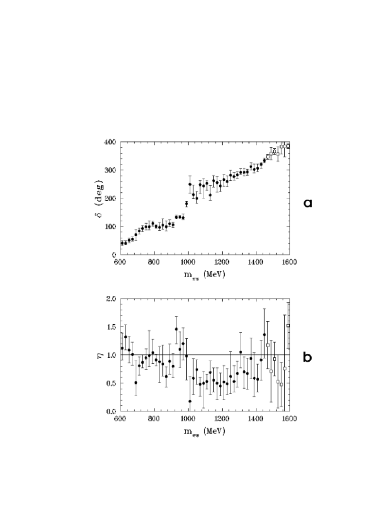
Figure 4: a) phase shifts $\delta$ and b) inelasticities $\eta$ for ”down-flat” solution (circles). Squares denote data from ref. [22].

It becomes clear from the errrors both in the phase shift ( figure 4 a ) as well as in the inelasticity ( figure 4 b ) that the details are, despite a remarkable effort in analysis, rather uncertain in the range of c.m. energies $600\ \mbox{MeV}\ \leq\ \sqrt{s}\ \leq\ 1600\ \mbox{MeV}$.

The red dragon and ”$\sigma$” in $\pi\pi\ ;\ I\ =\ 0$ s wave

The discussion of the partial wave amplitude, corresponding to the projection on $I\ =\ 0$ and on the s wave, denoted $t\ (\ q\ )$ in eq. 53

$$\begin{array}[]{l}t\ (\ q\ )\ =\ \left(\ S\ (\ q\ )\ -\ 1\ \right)\ /\ (\ 2\ i\ )\end{array}$$ (57)

has been the subject of many recent papers, to which we turn now. But we first show the result of combining elastic and quasi elastic pseudoscalar meson scattering, corresponding to the same quantum numbers, performed in ref. [5]. For a detailed discussion I refer back to ref. [5].

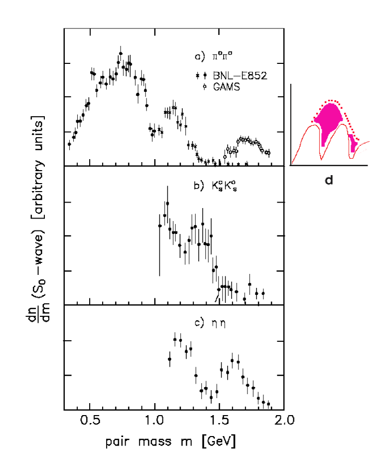
Figure 5: a) $\pi^{0}\ \pi^{0}$ , b) $K_{\ s}\ K_{\ s}$ , c) $\eta\ \eta$ , d) red dragon in full.

The absolute values $\left|\ t\ (\ q\ )\ \right|^{\ 2}$ (with only relative normalization) for $\pi\pi\ \rightarrow\ \pi\pi\ ,\ K\overline{K}\ ,\ \eta\eta$ are shown in figure 5 together with the full shape of the red dragon, amputating the negative interference due to $f_{\ 0}\ (\ 980\ )$ and $f_{\ 0}\ (\ 1500\ )$.

Several comments are necessary here :

i) ”data”

The compilation of figures 5 a - c makes it appear as if actual data is displayed. This is by no means the case, rather between the real data from the reactions

$$\begin{array}[]{l}\pi\ {\cal{N}}\ \rightarrow\ \left\{\ \begin{array}[]{l}\pi^{\ 0}\ \pi^{\ 0}\ {\cal{N}}\ (\ \Delta\ )\vspace*{0.3cm}\\ K_{\ s}\ K_{\ s}\ {\cal{N}}\ (\ \Delta\ )\vspace*{0.3cm}\\ \eta\ \eta\ {\cal{N}}\ (\ \Delta\ )\end{array}\right.\end{array}$$

and the displayed absolute values there is a series of analysis steps. The latter make it difficult to assess the overall errors.

ii) the second interference minimum due to $f_{\ 0}\ (\ 1500\ )$

The pattern showing two interfering narrow states : $f_{\ 0}\ (\ 980\ )$ and $f_{\ 0}\ (\ 1500\ )$ by todays notation, has been inferred from the peripheral $\pi\ {\cal{N}}$ reactions listed above.

The latter resonance has clearly been observed in $p\overline{p}$ annihilation at rest by the Crystal Barrel collaboration at the Lear facility of CERN [23] , adding a new element with high statistics and precision of analysis.

iii) the red dragon proper

The unfolding of the interference due to $f_{\ 0}\ (\ 980\ )$ and $f_{\ 0}\ (\ 1500\ )$ reveals a broad structure, the red dragon proper, as sketched in fig. 5 d.

The c.m. energy over which this structure is extended comprises the range $400\ \mbox{MeV}\ \leq\ \sqrt{s}\ \leq\ 1600\ \mbox{MeV}$ . Within all Breit-Wigner like strong interaction resonances, there does not exist a comparably wide one. This establishes the singular feature of the $\pi\pi$ s wave scattering amplitude in this range, and also considerably below 400 MeV, i.e. down to the two pion threshold, as well as above 1600 MeV.

The combined experimental and theoretical evaluation of data, which led to the clear picture represented by the red dragon in figure 5 is not subject to the remaining large inherent errors of details of the respective scattering amplitudes. This contrasts with all attempts : [5] , [19] and those discussed below, where further interpretation of details of the red dragon are undertaken.

$\sigma\ (\ \sim\ 500\ )$ and/or $\kappa\ (\ \sim\ 750\ )$ scalar mesons

The claims of the existence of an isospin singlet, nonstrange scalar state $\sigma$ in a mass region clearly below $f_{\ 0}\ (\ 980\ )$ are numerous besides ref. [19]. Another light scalar state, $\kappa$ with isospin 1/2, well below $K^{\ *}_{\ 0}\ (\ 1430\ )$ has also received much attention. These claims have been recently repeated on various grounds. We cite two reviews compiled within the PDG [13] : on scalar mesons [24] and on non $q\overline{q}$ candidates [25] .

A new window has opened up in the study of the decay of charmed [26] , [27] and b flavored mesons [28] , [29] .

What is emerging from c- and b-flavored meson decays is the clear fact, that in three pseudoscalar meson ( $\pi$ and $K$ ) decays two out of the three pseudoscalars are produced amply in their relative s wave. This is quite in line with analogous decays from $p\overline{p}$ and hence the analysis in terms of two body amplitudes, the third pseudoscalar beeing treated as ’kinematical spectator, modulo constraints from Bose statistics’, was performed in all reactions in a similar way.

A few decays are listed below for definiteness

$$\begin{array}[]{lll ll}\begin{array}[]{l}D^{\ +}\vspace*{0.3cm}\\ D^{\ +}_{\ s}\end{array}&\rightarrow&\hskip 8.5359pt\pi^{\ -}\ \pi^{\ +}\ \pi^{\ +}&;&\hskip 8.5359pt\cite[cite]{[\@@bibref{}{aitala}{}{}]}\ ,\ \cite[cite]{[\@@bibref{}{bediaga}{}{}]}\vspace*{0.3cm}\\ B^{\ +}&\rightarrow&\ \begin{array}[]{l}\pi^{\ -}\ K^{\ +}\ \pi^{\ +}\vspace*{0.3cm}\\ K^{\ -}\ K^{\ +}\ K^{\ +}\end{array}&;&\hskip 8.5359pt\cite[cite]{[\@@bibref{}{garmash}{}{}]}\ ,\ \cite[cite]{[\@@bibref{}{babar}{}{}]}\vspace*{0.3cm}\\ p\ \overline{p}&\rightarrow&\hskip 8.5359pt\pi^{\ -}\ \pi^{\ +}\ \eta&;&\hskip 8.5359pt\cite[cite]{[\@@bibref{}{amslerrev2}{}{}]}\end{array}$$ (58)

The present results from the study of the above decays do favour the derived existence of a ’$\sigma$’ isoscalar state, called $f_{\ 0}\ (\ 600\ )$ by the PDG [13] as well as indications of an isospin 1/2 state called ’$\kappa$’, with masses $\sim\ 500$ MeV for $\sigma$ and $\sim\ 750$ MeV for $\kappa$ respectively. The determination of the widths is rather uncertain, but follows the widths of peaks in the projected Dalitz plot distributions of the order of 200-400 MeV.

It is fair to say, that as welcome as these new channels are, the present stage of analysis has not led to a clear picture of scalar meson states.

c) Central production experiments

The first experiment searching for gluonic mesons in central production was performed at the ISR at CERN [31] , at $\sqrt{s}\ =\ 63$ GeV.

I reproduce here the invariant mass distribution of $\pi^{\ +}\ \pi^{\ -}$ pairs as observed in ref. [31]

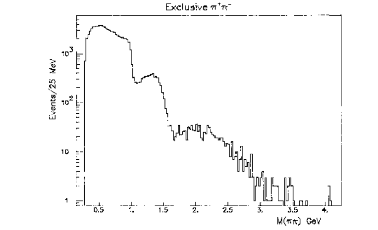
Figure 6: Invariant mass distribution of $\pi^{\ \pm}$ pairs in central $p\ p\ \rightarrow\ p\ p\ X_{\ c}$ production at $\sqrt{s}\ =\ 63$ GeV [31].

Even though figure 6 represents the (absolute) square of an amplitude and figure 5 the square of another amplitude, the similarity and shape of the red dragon is clearly visible. This similarity does not need any further analysis.

The more recent experiment WA102 and its predecessor WA76 are using a fixed target configuration and thus the c.m. energies studied are lower $\sqrt{s}\ \leq\ 29$ GeV [32] .

Despite dedicated studies [33], no clear understanding of central production and spectroscopic information encoded in ps-ps scattering amplitudes ( section b) of this chapter ) nor any convincing evidence for the mass region from lattice QCD calculations ( section a) of this chapter ) for the gluonic binary $gb(\ 0^{\ ++}\ )$ is emerging.

Rather a choice of apparent possibilities is offered, where in order not to offend any individuals I follow the PDG [13]

$$\begin{array}[]{l}f_{\ 0}\ :\ 600\ ,\ 980\ ,\ 1370\ ,\ 1500\ ,\ 1710\ \cdots\ \mbox{MeV}\end{array}$$ (59)

The present controversial situation does - in my opinion - reflect human shortcomings more than intrinsic difficulty to understand the strong interaction dynamics underlying gluonic binaries as well as $q\ \overline{q}$ scalar mesons.

5 Conclusion

In view of the previous sentence and in summary of the present outline, I think that a dedicated experiment of central production, at the highest achievable c.m. energies as well as with an optimally adapted detector is scientifically worth while.

Appendix A Appendix

A.1 Spinor wave functions, spin states and transformation rules

We present the spin 1/2 chiral building blocks below, as they determine the general spin transformation rules defined in eq. (13) .

$$\begin{array}[]{l}S_{\ \underline{\alpha}}^{\hskip 8.5359pt\underline{\beta}}\ (\ a\ )\ =\ \left\{\ S_{\ \alpha_{1}}^{\hskip 8.5359pt\beta_{1}}\ (\ a\ )\ \times\ \cdots\ \times\ S_{\ \alpha_{N}}^{\hskip 8.5359pt\beta_{N}}\ (\ a\ )\ \right\}_{\ symm}\end{array}$$ (60)

The irreducible blocks $S_{\ \alpha_{j}}^{\hskip 8.5359pt\beta_{j}}\ (\ a\ )$ in eq. (60) correspond to spin 1/2

$$\begin{array}[]{l}a\ =\ \left(\ a_{\ 0}\ ,\ a_{\ 1}\ ,\ a_{\ 2}\ ,\ a_{\ 3}\ \right)\ =\ a_{\ \mu}\hskip 8.5359pt:\hskip 8.5359pt\begin{array}[]{l}\mbox{complex four-vector}\vspace*{0.1cm}\\ \mbox{{\it not} a Lorentz vector}\end{array}\vspace*{0.3cm}\\ S_{\ \alpha}^{\hskip 8.5359pt\beta}\ (\ a\ )\ =\ S_{\ 1}^{\ 1}\ (\ a\ )\ =\ \left(\ a_{\ 0}\ \Sigma_{\ 0}\ +\ \frac{1}{i}\ \vec{a}\ \vec{\Sigma}\ \right)_{\ \alpha}^{\hskip 8.5359pt\beta}\vspace*{0.3cm}\\ S_{\ 1}^{\ 1}\ (\ a\ )\ =\ \left(\begin{array}[]{rr}a_{\ 0}\ -\ i\ a_{\ 3}&\hskip 5.69046pt-\ a_{\ 2}\ -\ i\ a_{\ 1}\vspace*{0.3cm}\\ a_{\ 2}\ -\ i\ a_{\ 1}&\hskip 5.69046pta_{\ 0}\ +\ i\ a_{\ 3}\end{array}\ \right)\vspace*{0.3cm}\\ a^{\ 2}\ =\ a_{\ 0}^{\ 2}\ +\ \vec{a}^{\ 2}\ =\ Det\ S_{\ 1}^{\ 1}\ =\ 1\end{array}$$ (61)

The quadratic constraint restricts $S_{\ 1}^{\ 1}$ as defined in eq. 61 to be unimodular (i.e. to have Det = 1). Rotations ( by half angles in bosonic terms ) correspond to $a_{\ \mu}$ real. This is parametrizing the sphere ( over the real numbers ) : $S_{\ 3}\ \equiv\ SU2$. Lorentz boosts ( by hyperbolic half angles in bosonic terms ) correspond to $a_{\ 0}$ real, $\vec{a}$ pure imaginary. This is parametrizing the double hyperboloid ( over the real numbers ) : $(\ \Re\ a_{\ 0}\ )^{\ 2}\ -\ (\ \Im\ \vec{a}\ )^{\ 2}\ =\ 1$.

The matrices $\Sigma_{\ 0}\ ,\ \Sigma_{\ k}\ ;\ k=\ 1,2,3$ are the Pauli matrices, as arising in the right chiral representation of the full $\gamma\ -$ matrix algebra.

$$\begin{array}[]{l}\left(\ \sigma_{\ \mu\ \nu}\ \right)_{\ \alpha}^{\hskip 8.5359pt\beta}\ \leftrightarrow\ P_{\ R}\ \frac{i}{2}\ \left[\ \gamma_{\ \mu}\ ,\ \gamma_{\ \nu}\ \right]\ P_{\ R}\hskip 8.5359pt;\hskip 8.5359ptP_{\ R}\ =\ \frac{1}{2}\ (\ 1\ +\ \gamma_{\ 5\ R}\ )\vspace*{0.3cm}\\ \gamma_{\ 5\ R}\ =\ \frac{1}{i}\ \gamma_{\ 0}\ \gamma_{\ 1}\ \gamma_{\ 2}\ \gamma_{\ 3}\vspace*{0.3cm}\\ \left(\ \sigma_{\ \mu\ \nu}\ \right)_{\ \alpha}^{\hskip 8.5359pt\beta}\ =\ \begin{array}[]{ll}\ \left(\begin{array}[]{l}-\ i\ \Sigma_{\ k}\vspace*{0.3cm}\\ \varepsilon_{\ mnr}\ \Sigma_{\ r}\end{array}\ \right)_{\alpha}^{\hskip 8.5359pt\beta}\vspace*{1.0cm}&\vspace*{-0.5cm}\begin{array}[]{l}\mbox{for}\ \mu\ =\ 0\ ,\ \nu\ =\ k\ =\ 1,2,3\vspace*{0.3cm}\\ \mbox{for}\ \mu\ =\ m\ ,\ \nu\ =\ n\ ;\vspace*{-0.2cm}\\ \hskip 76.82234ptm,n,r\ =\ 1,2,3\end{array}\end{array}\end{array}$$ (62)

The right chiral quantities $\left(\ \sigma_{\ \mu\ \nu}\ \right)_{\ \alpha}^{\hskip 8.5359pt\beta}$ in eq. (62) satisfy the duality relation

$$\begin{array}[]{l}\left(\ \sigma_{\ \mu\ \nu}\ \right)_{\ \alpha}^{\hskip 8.5359pt\beta}\ \rightarrow\ \sigma_{\ \mu\ \nu}^{\ R}\hskip 8.5359pt;\hskip 8.5359pt\sigma_{\ \mu\ \nu}^{\ R}\ =\ -\ i\ \frac{1}{2}\ \varepsilon_{\ \mu\nu\varrho\tau}\ \sigma^{\ \varrho\ \tau\ R}\end{array}$$ (63)

Half angles (6) , rotational and hyperbolic - a) to the right

An infinitesimal Lorentz transformation is covered by the spin 1/2 half angles $\omega^{\ \mu\nu}$ , defined below, multiplying the (right chiral) base transformations $\sigma_{\ \mu\ \nu}^{\ R}$

$$\begin{array}[]{l}\omega^{\ \mu\nu}\ =\ \frac{1}{2}\ \Omega^{\ \mu\nu}\vspace*{0.3cm}\\ \omega^{\ \mu\nu}\ =\ \left(\begin{array}[]{ccc c}0&\varepsilon_{\ 1}&\varepsilon_{\ 2}&\varepsilon_{\ 3}\vspace*{0.1cm}\\ -\varepsilon_{\ 1}&0&\Theta_{\ 3}&-\Theta_{\ 2}\vspace*{0.1cm}\\ -\varepsilon_{\ 2}&-\Theta_{\ 3}&0&\Theta_{\ 1}\vspace*{0.1cm}\\ -\varepsilon_{\ 3}&\Theta_{\ 2}&-\Theta_{\ 1}&0\end{array}\ \right)\ =\ \omega^{\ \mu\nu}\ (\ \vec{\Theta}\ ,\ \vec{\varepsilon}\ )\end{array}$$ (64)

Projecting $\omega$ onto $\sigma^{\ R}$ we obtain

$$\begin{array}[]{l}\left(\ \omega^{\ R}\ \right)_{\ \alpha}^{\hskip 8.5359pt\beta}\hskip 8.5359pt\rightarrow\hskip 8.5359pt\omega_{\ \alpha}^{\hskip 8.5359pt\beta}\vspace*{0.3cm}\\ \omega_{\ \alpha}^{\hskip 8.5359pt\beta}\ =\ \frac{1}{2}\ \omega^{\ \mu\nu}\ \left(\ \sigma_{\ \mu\ \nu}\ \right)_{\ \alpha}^{\hskip 8.5359pt\beta}\ =\ i\ \left(\ \left\{\ \vec{\Theta}\ -i\ \vec{\varepsilon}\ \right\}\ \frac{1}{i}\ \vec{\Sigma}\ \right)_{\ \alpha}^{\hskip 8.5359pt\beta}\vspace*{0.3cm}\\ \rightarrow\ \vec{\omega}\ \equiv\ \vec{\omega}^{\ R}\ =\ \vec{\Theta}\ -\ i\ \vec{\varepsilon}\end{array}$$ (65)

$S_{\ 1}^{\ 1}$ in eq. (61) then represents the exponential of $\left(\ \omega\ \right)_{\ \alpha}^{\hskip 8.5359pt\beta}$ (multiplied with $\frac{1}{i}$)

$$\begin{array}[]{l}S_{\ \alpha}^{\hskip 8.5359pt\beta}\ (\ a\ )\ =\ \exp\ \left(\ \frac{1}{i}\ \omega\ \right)_{\ \alpha}^{\hskip 8.5359pt\beta}\ =\ \exp\ \left(\ \frac{1}{i}\ \vec{\omega}\ \vec{\Sigma}\ \right)_{\ \alpha}^{\hskip 8.5359pt\beta}\end{array}$$ (66)

Leaving out the (right chiral) spinor indices eq. (66) becomes

$$\begin{array}[]{l}S\ (\ a\ )\ =\ \cos\ (\ \vec{\omega}\ \vec{\Sigma}\ )\ -\ i\ \sin\ (\ \vec{\omega}\ \vec{\Sigma}\ )\end{array}$$ (67)

Thus we introduce the orthogonal complex invariant of $\vec{\omega}$

$$\begin{array}[]{l}Z\ (\ \omega\ )\ =\ z^{\ 2}\ (\ \omega\ )\ =\ \vec{\omega}^{\ 2}\ =\ \left\{\ \vec{\Theta}^{\ 2}\ -\ \vec{\varepsilon}^{\ 2}\ \right\}\ -\ i\ \left\{\ 2\ \vec{\Theta}\ \vec{\varepsilon}\ \right\}\vspace*{0.3cm}\\ \rightarrow\hskip 8.5359ptS\ (\ a\ )\ =\ \cos\ (\ z\ )\ \Sigma_{\ 0}\ -\ i\ \left[\ \sin\ (\ z\ )\ /\ z\ \right]\ \vec{\omega}\ \vec{\Sigma}\vspace*{0.3cm}\\ \hskip 8.5359pta\ =\ a\ (\ \omega\ )\hskip 8.5359pt;\hskip 8.5359pta_{\ 0}\ =\ \cos\ (\ z\ )\hskip 8.5359pt;\hskip 8.5359pt\vec{a}\ =\ \left[\ \sin\ (\ z\ )\ /\ z\ \right]\ \vec{\omega}\end{array}$$ (68)

The square root ambiguity of $z\ (\ \omega\ )\ =\ \pm\ \sqrt{Z\ (\ \omega\ )}$ does not affect the functional relation $a\ =\ a\ (\ \omega\ )$, as becomes clear from eq. (68).

From right chiral to left chiral spinors

The right chiral base representations of $SL2C_{\ R}$ are by construction not parity invariant, nor are the matrices $S\ (\ a\ )\ \equiv\ {\cal{A}}$ over the real numbers.

Se we shall transform the defining equations (60-62) to the left chiral side

$$\begin{array}[]{l}\hskip 17.07182ptS_{\ \underline{\alpha}}^{\hskip 8.5359pt\underline{\beta}}\ (\ a\ )\ =\ \left\{\ S_{\ \alpha_{1}}^{\hskip 8.5359pt\beta_{1}}\ (\ a\ )\ \times\ \cdots\ \times\ S_{\ \alpha_{N}}^{\hskip 8.5359pt\beta_{N}}\ (\ a\ )\ \right\}_{\ symm}\ \rightarrow\vspace*{0.3cm}\\ \rightarrow\ \widetilde{S}^{\ \underline{\dot{\gamma}}}_{\hskip 8.5359pt\underline{\dot{\delta}}}\ (\ b\ )\ =\ \left\{\ \widetilde{S}^{\ \dot{\gamma}_{1}}_{\hskip 8.5359pt\dot{\delta}_{1}}\ (\ b\ )\ \times\ \cdots\ \times\ \widetilde{S}^{\ \dot{\gamma}_{N}}_{\hskip 8.5359pt\dot{\delta}_{N}}\ (\ b\ )\ \right\}_{\ symm}\end{array}$$ (69)

$$\begin{array}[]{l}b\ =\ \left(\ b_{\ 0}\ ,\ b_{\ 1}\ ,\ b_{\ 2}\ ,\ b_{\ 3}\ \right)\ =\ b_{\ \mu}\hskip 8.5359pt:\hskip 8.5359pt\begin{array}[]{l}\mbox{complex four-vector}\vspace*{0.1cm}\\ \mbox{{\it not} a Lorentz vector}\end{array}\vspace*{0.3cm}\\ \widetilde{S}^{\ \dot{\gamma}}_{\hskip 8.5359pt\dot{\delta}}\ (\ b\ )\ =\ \widetilde{S}_{\ 2}^{\ 2}\ (\ b\ )\ =\ \left(\ b_{\ 0}\ \widetilde{\Sigma}_{\ 0}\ +\ \frac{1}{i}\ \vec{b}\ \vec{\widetilde{\Sigma}}\ \right)^{\ \dot{\gamma}}_{\hskip 8.5359pt\dot{\delta}}\vspace*{0.3cm}\\ \widetilde{S}_{\ 2}^{\ 2}\ (\ b\ )\ =\ \left(\begin{array}[]{rr}b_{\ 0}\ -\ i\ b_{\ 3}&\hskip 5.69046pt-\ b_{\ 2}\ -\ i\ b_{\ 1}\vspace*{0.3cm}\\ b_{\ 2}\ -\ i\ b_{\ 1}&\hskip 5.69046ptb_{\ 0}\ +\ i\ b_{\ 3}\end{array}\ \right)\vspace*{0.3cm}\\ b^{\ 2}\ =\ b_{\ 0}^{\ 2}\ +\ \vec{b}^{\ 2}\ =\ Det\ \widetilde{S}_{\ 2}^{\ 2}\ =\ 1\end{array}$$ (70)

The transformation from ${\cal{A}}$ to ${\cal{B}}$ corresponds to the substitution

$$\begin{array}[]{l}{\cal{A}}\ \rightarrow\ \left(\ {\cal{A}}^{\ \dagger}\ \right)^{\ -1}\ =\ {\cal{B}}\end{array}$$ (71)

The substitution in eq. (71) makes use of the four base representations of SL2C, best represented in the associated quadrangle

$$\begin{array}[]{l}\begin{array}[]{ccc}{\cal{A}}&\longleftrightarrow&\left(\ {\cal{A}}^{\ T}\ \right)^{\ -1}\vspace*{0.3cm}\\ \updownarrow\ \equiv\ c.c.&&\updownarrow\ \equiv\ c.c.\vspace*{0.3cm}\\ \overline{\cal{A}}&\longleftrightarrow&\left(\ {\cal{A}}^{\ \dagger}\ \right)^{\ -1}\end{array}\end{array}$$ (72)

In the quadrangle in eq. (72) the up-down operation means complex conjugation of each matrix element, forming the involutory chains

$$\begin{array}[]{c}{\cal{A}}\ \rightarrow\ \overline{{\cal{A}}}\ \rightarrow\ {\cal{A\vspace*{0.3cm}}}\\ \mbox{and}\vspace*{0.3cm}\\ \left(\ {\cal{A}}^{\ T}\ \right)^{\ -1}\ \rightarrow\ \left(\ {\cal{A}}^{\ \dagger}\ \right)^{\ -1}\ \rightarrow\ \left(\ {\cal{A}}^{\ T}\ \right)^{\ -1}\end{array}$$

whereas the left-right operation associates the symplectic dual, forming the equally involutary chains

$$\begin{array}[]{c}{\cal{A}}\ \rightarrow\ \left(\ {\cal{A}}^{\ T}\ \right)^{\ -1}\ \rightarrow\ {\cal{A\vspace*{0.3cm}}}\\ \mbox{and}\vspace*{0.3cm}\\ \overline{{\cal{A}}}\ \rightarrow\ \left(\ {\cal{A}}^{\ \dagger}\ \right)^{\ -1}\ \rightarrow\ \overline{{\cal{A}}}\end{array}$$

Thus both up-down and left-right transformations along the quadrangle in eq. (72) are commutative as well as involutory.

Yet the left-right transformation associates equivalent representations, contrary to the up- down one, which associates inequivalent representations, of which we have chosen the two residing in the upper left and lower right corners of the triangle in eq. (72.

The symplectic equivalence is realized in the right chiral basis by

$$\begin{array}[]{l}\left(\ {\cal{A}}^{\ T}\ \right)^{\ -1}\ =\ s\ {\cal{A}}\ s^{\ -1}\hskip 8.5359pt;\hskip 8.5359pts\ =\ (\ \pm\ )\ i\ \sigma_{\ 2}\ =\ (\ \pm\ )\ \left(\begin{array}[]{rl}0&1\vspace*{0.2cm}\\ -1&0\end{array}\right)\end{array}$$ (73)

The base Pauli matrices go into each other under the substitution in eq. (71)

$$\begin{array}[]{l}\Sigma_{\ \mu}\ =\ \Sigma_{\ \mu}^{\ \dagger}\ =\ \left(\ \Sigma_{\ \mu}\ \right)^{\ -1}\ =\ \left(\ \Sigma_{\ \mu}^{\ \dagger}\ \right)^{\ -1}\vspace*{0.2cm}\\ \rightarrow\ \left(\ \widetilde{\Sigma}_{\ 0}\ ,\ \vec{\widetilde{\Sigma}}\ \right)\ =\ \left(\ \Sigma_{\ 0}\ ,\ \vec{\Sigma}\ \right)\end{array}$$ (74)

Hence we have

$$\begin{array}[]{l}{\cal{A}}\ \rightarrow\ \left(\ {\cal{A}}^{\ \dagger}\ \right)^{\ -1}\ =\ {\cal{B}}\ (\ {\cal{A}}\ )\vspace*{0.3cm}\\ b\ =\ \overline{a}\hskip 8.5359pt;\hskip 8.5359pt\forall\ \mbox{components}\end{array}$$ (75)

Thus the quadrangle in eq. (72) leads to the right- and left-chiral reality restricted form of $SL2C_{\ R}\ \times\ SL2C_{\ L}$

$$\begin{array}[]{l}\left\{spin\right\}\ \rightarrow\ s\hskip 8.5359pt,\hskip 8.5359pt\#\ s\ =\ N\ +\ 1\hskip 8.5359pt;\hskip 8.5359ptD_{\ s\ s^{{}^{\prime}}}\ =\ D_{\ s\ s^{{}^{\prime}}}^{\ J}\ (\ \Lambda\ ,\ p\ )\vspace*{0.5cm}\\ \begin{array}[]{lll lll l}R&:&t_{\ \underline{\alpha}}\ (\ \Lambda p\ ;\ s\ )&=&S_{\ \underline{\alpha}}^{\hskip 8.5359pt\underline{\beta}}\ (\ a\ )&\hskip 5.69046ptt_{\ \underline{\beta}}\ (\ p\ ;\ s^{{}^{\prime}}\ )&\hskip 5.69046ptD_{\ s\ s^{{}^{\prime}}}\vspace*{0.3cm}\\ L&:&\widetilde{t}^{\ \underline{\dot{\gamma}}}\ (\ \Lambda p\ ;\ s\ )&=&\widetilde{S}^{\ \underline{\dot{\gamma}}}_{\hskip 11.38092pt\underline{\dot{\delta}}}\ (\ b\ )&\hskip 5.69046pt\widetilde{t}^{\ \underline{\dot{\delta}}}\ (\ p\ ;\ s^{{}^{\prime}}\ )&\hskip 5.69046ptD_{\ s\ s^{{}^{\prime}}}\end{array}\end{array}$$ (76)

While we proceed in steps, let me quote Res Jost [34] , illustrating the L-R chiral aspects.

The decomposition in eq. (60) expands (doubles) into

$$\begin{array}[]{l}\begin{array}[]{lll}R&:&S_{\ \underline{\alpha}}^{\hskip 8.5359pt\underline{\beta}}\ (\ a\ )\ =\ \left\{\ S_{\ \alpha_{1}}^{\hskip 8.5359pt\beta_{1}}\ (\ a\ )\ \times\ \cdots\ \times\ S_{\ \alpha_{N}}^{\hskip 8.5359pt\beta_{N}}\ (\ a\ )\ \right\}_{\ symm}\vspace*{0.3cm}\\ L&:&\widetilde{S}^{\ \underline{\dot{\gamma}}}_{\hskip 11.38092pt\underline{\dot{\delta}}}\ (\ b\ )\ =\ \left\{\ \widetilde{S}^{\ \dot{\gamma_{1}}}_{\hskip 11.38092pt\dot{\delta_{1}}}\ (\ b\ )\ \times\ \cdots\ \times\ \widetilde{S}^{\ \dot{\gamma_{N}}}_{\hskip 11.38092pt\dot{\delta_{N}}}\ (\ b\ )\ \right\}_{\ symm}\end{array}\end{array}$$ (77)

and then reduces to the R-L spin 1/2 building blocks

$$\begin{array}[]{l}\begin{array}[]{lll ll ll}R&:&S_{\ \alpha}^{\hskip 8.5359pt\beta}\ (\ a\ )&=&S_{\ 1}^{\ 1}\ (\ a\ )\ \equiv\ {\cal{A}}\ (\ a\ )&=&\left(\ a_{\ 0}\ \Sigma_{\ 0}\ +\ \frac{1}{i}\ \vec{a}\ \vec{\Sigma}\ \right)_{\ \alpha}^{\hskip 8.5359pt\beta}\vspace*{0.3cm}\\ L&:&\widetilde{S}^{\ \dot{\gamma}}_{\hskip 8.5359pt\dot{\delta}}\ (\ b\ )&=&\widetilde{S}_{\ 2}^{\ 2}\ (\ b\ )\ \equiv\ {\cal{B}}\ (\ b\ )&=&\left(\ b_{\ 0}\ \widetilde{\Sigma}_{\ 0}\ +\ \frac{1}{i}\ \vec{b}\ \vec{\widetilde{\Sigma}}\ \right)^{\ \dot{\gamma}}_{\hskip 8.5359pt\dot{\delta}}\end{array}\vspace*{0.3cm}\\ \widetilde{\Sigma}_{\ \mu}\ =\ \Sigma_{\ \mu}\end{array}$$ (78)

The reality condition corresponds to a diagonal in the quadrangle in eq. (72)

$$\begin{array}[]{l}\begin{array}[]{rcr c}{\cal{A}}\ (\ a\ )&\longleftrightarrow&{\cal{B}}\ (\ b\ )&\vspace*{-0.1cm}\hfil\\ \searrow&&\searrow&\vspace*{-0.0cm}\hfil\\ &{\cal{A}}&=&\left(\ {\cal{B}}^{\ \dagger}\ \right)^{\ -1}\vspace*{-0.1cm}\\ &\downarrow&&\downarrow\vspace*{-0.0cm}\\ &a&=&\overline{b}\end{array}\end{array}$$ (79)

The so constrained pair

$$\begin{array}[]{l}\left(\ {\cal{A}}\ (\ a\ )\ ,\ {\cal{B}}\ (\ \overline{a}\ )\ \right)\ \equiv\ spin\ (\ 1\ ,\ 3\ ;\ \Re\ )\ \simeq\ SL2C\end{array}$$ (80)

defines the (self covered) group $spin\ (\ 1\ ,\ 3\ ;\ \Re\ )$ : $\Re$ indicates that the spin group is over the real numbers, whereas $1\ ,\ 3$ denote the signature of the derived metric, i.e. 1 time and 3 space (real) dimensions.

Half angles (6) , rotational and hyperbolic - b) to the left

The left-chiral representation of $spin\ (\ 1\ ,\ 3\ ;\ \Re\ )$ complements the right-chiral one defined in eq. (62)

$$\begin{array}[]{l}\left(\ \sigma_{\ \mu\ \nu}\ \right)^{\ \dot{\gamma}}_{\hskip 11.38092pt\dot{\delta}}\ \leftrightarrow\ P_{\ L}\ \frac{i}{2}\ \left[\ \gamma_{\ \mu}\ ,\ \gamma_{\ \nu}\ \right]\ P_{\ L}\hskip 8.5359pt;\hskip 8.5359ptP_{\ L}\ =\ \frac{1}{2}\ (\ 1\ -\ \gamma_{\ 5\ R}\ )\vspace*{0.3cm}\\ \gamma_{\ 5\ R}\ =\ \frac{1}{i}\ \gamma_{\ 0}\ \gamma_{\ 1}\ \gamma_{\ 2}\ \gamma_{\ 3}\vspace*{0.3cm}\\ \left(\ \sigma_{\ \mu\ \nu}\ \right)^{\ \dot{\gamma}}_{\hskip 11.38092pt\dot{\delta}}\ =\ \begin{array}[]{ll}\ \left(\begin{array}[]{l}i\ \Sigma_{\ k}\vspace*{0.3cm}\\ \varepsilon_{\ mnr}\ \Sigma_{\ r}\end{array}\ \right)^{\dot{\gamma}}_{\hskip 11.38092pt\dot{\delta}}\vspace*{1.0cm}&\vspace*{-0.5cm}\begin{array}[]{l}\mbox{for}\ \mu\ =\ 0\ ,\ \nu\ =\ k\ =\ 1,2,3\vspace*{0.3cm}\\ \mbox{for}\ \mu\ =\ m\ ,\ \nu\ =\ n\ ;\vspace*{-0.2cm}\\ \hskip 76.82234ptm,n,r\ =\ 1,2,3\end{array}\end{array}\end{array}$$ (81)

In principle we should have distinguished the left chiral matrices $\widetilde{\Sigma}_{\ \mu}$ characterizing the left chiral SL2C basis in eq. (81) but we have chosen (without loss of generality) to identify $\widetilde{\Sigma}_{\ \mu}\ =\ \Sigma_{\ \mu}$ as specified in eq. (78).

The left chiral variant of eq. (63) becomes

$$\begin{array}[]{l}\left(\ \sigma_{\ \mu\ \nu}\ \right)_{\ \alpha}^{\hskip 8.5359pt\beta}\ \rightarrow\ \sigma_{\ \mu\ \nu}^{\ R}\hskip 8.5359pt;\hskip 8.5359pt\sigma_{\ \mu\ \nu}^{\ R}\ =\ -\ i\ \frac{1}{2}\ \varepsilon_{\ \mu\nu\varrho\tau}\ \sigma^{\ \varrho\ \tau\ R}\vspace*{0.3cm}\\ \rightarrow\ \left(\ \sigma_{\ \mu\ \nu}\ \right)^{\ \dot{\gamma}}_{\hskip 11.38092pt\dot{\delta}}\ \rightarrow\ \sigma_{\ \mu\ \nu}^{\ L}\hskip 8.5359pt;\hskip 8.5359pt\sigma_{\ \mu\ \nu}^{\ L}\ =\ +\ i\ \frac{1}{2}\ \varepsilon_{\ \mu\nu\varrho\tau}\ \sigma^{\ \varrho\ \tau\ L}\end{array}$$ (82)

Eq. (65) when reflected to the left takes on the form

$$\begin{array}[]{l}\left(\ \omega^{\ L}\ \right)^{\ \dot{\gamma}}_{\hskip 11.38092pt\dot{\delta}}\hskip 8.5359pt\rightarrow\hskip 8.5359pt\widetilde{\omega}^{\ \dot{\gamma}}_{\hskip 11.38092pt\dot{\delta}}\vspace*{0.3cm}\\ \widetilde{\omega}^{\ \dot{\gamma}}_{\hskip 11.38092pt\dot{\delta}}\ =\ \frac{1}{2}\ \omega^{\ \mu\nu}\ \left(\ \sigma_{\ \mu\ \nu}\ \right)^{\ \dot{\gamma}}_{\hskip 11.38092pt\dot{\delta}}\ =\ i\ \left(\ \left\{\ \vec{\Theta}\ +i\ \vec{\varepsilon}\ \right\}\ \frac{1}{i}\ \vec{\Sigma}\ \right)^{\ \dot{\gamma}}_{\hskip 11.38092pt\dot{\delta}}\vspace*{0.3cm}\\ \rightarrow\ \vec{\widetilde{\omega}}\ \equiv\ \vec{\omega}^{\ L}\ =\ \vec{\Theta}\ +\ i\ \vec{\varepsilon}\hskip 8.5359pt;\hskip 8.5359pt\vec{\omega}\ \equiv\ \vec{\omega}^{\ R}\ =\ \vec{\Theta}\ -\ i\ \vec{\varepsilon}\end{array}$$ (83)

$\widetilde{S}_{\ 2}^{\ 2}$ in eq. (78 is along with the right counterpart in eq. (66)

$$\begin{array}[]{l}S_{\ \alpha}^{\hskip 8.5359pt\beta}\ (\ a\ )\ =\ \exp\ \left(\ \frac{1}{i}\ \omega\ \right)_{\ \alpha}^{\hskip 8.5359pt\beta}\ =\ \exp\ \left(\ \frac{1}{i}\ \vec{\omega}\ \vec{\Sigma}\ \right)_{\ \alpha}^{\hskip 8.5359pt\beta}\vspace*{0.3cm}\\ \rightarrow\ \widetilde{S}^{\ \dot{\gamma}}_{\hskip 8.5359pt\dot{\delta}}\ (\ b\ )\ =\ \exp\ \left(\ \frac{1}{i}\ \widetilde{\omega}\ \right)^{\ \dot{\gamma}}_{\hskip 11.38092pt\dot{\delta}}\ =\ \exp\ \left(\ \frac{1}{i}\ \vec{\widetilde{\omega}}\ \vec{\Sigma}\ \right)^{\ \dot{\gamma}}_{\hskip 11.38092pt\dot{\delta}}\end{array}$$ (84)

Eq. (67) extends to

$$\begin{array}[]{l}S\ (\ a\ )\ =\ \cos\ (\ \vec{\omega}\ \vec{\Sigma}\ )\ -\ i\ \sin\ (\ \vec{\omega}\ \vec{\Sigma}\ )\vspace*{0.3cm}\\ \rightarrow\ \widetilde{S}\ (\ b\ )\ =\ S\ (\ b\ )\ =\ \exp\ \left(\ \frac{1}{i}\ \widetilde{\omega}\ \right)\ =\ \cos\ (\ \vec{\widetilde{\omega}}\ \vec{\Sigma}\ )\ -\ i\ \sin\ (\ \vec{\widetilde{\omega}}\ \vec{\Sigma}\ )\vspace*{0.3cm}\\ \hskip 14.22636pt\vec{\widetilde{\omega}}\ =\ \overline{\vec{\omega}}\hskip 8.5359pt;\hskip 8.5359ptb\ =\ \overline{a}\vspace*{0.3cm}\\ \hskip 14.22636ptS\ (\ a\ )\ =\ a_{\ 0}\ \Sigma_{\ 0}\ +\ \frac{1}{i}\ \vec{a}\ \vec{\Sigma}\hskip 8.5359pt;\hskip 8.5359ptS\ (\ b\ )\ =\ b_{\ 0}\ \Sigma_{\ 0}\ +\ \frac{1}{i}\ \vec{b}\ \vec{\Sigma}\end{array}$$ (85)

Eq. (68) completes to

$$\begin{array}[]{l}Z\ (\ \omega\ )\ =\ z^{\ 2}\ (\ \omega\ )\ =\ \vec{\omega}^{\ 2}\ =\ \left\{\ \vec{\Theta}^{\ 2}\ -\ \vec{\varepsilon}^{\ 2}\ \right\}\ -\ i\ \left\{\ 2\ \vec{\Theta}\ \vec{\varepsilon}\ \right\}\vspace*{0.3cm}\\ \rightarrow\hskip 8.5359ptS\ (\ a\ )\ =\ \cos\ (\ z\ )\ \Sigma_{\ 0}\ -\ i\ \left[\ \sin\ (\ z\ )\ /\ z\ \right]\ \vec{\omega}\ \vec{\Sigma}\vspace*{0.3cm}\\ \hskip 8.5359pta\ =\ a\ (\ \omega\ )\hskip 8.5359pt;\hskip 8.5359pta_{\ 0}\ =\ \cos\ (\ z\ )\hskip 8.5359pt;\hskip 8.5359pt\vec{a}\ =\ \left[\ \sin\ (\ z\ )\ /\ z\ \right]\ \vec{\omega}\vspace*{0.5cm}\\ \rightarrow\hskip 8.5359ptZ\ (\ \widetilde{\omega}\ )\ =\ z^{\ 2}\ (\ \widetilde{\omega}\ )\ =\ \vec{\widetilde{\omega}}^{\ 2}\ =\ \left\{\ \vec{\Theta}^{\ 2}\ -\ \vec{\varepsilon}^{\ 2}\ \right\}\ +\ i\ \left\{\ 2\ \vec{\Theta}\ \vec{\varepsilon}\ \right\}\vspace*{0.3cm}\\ Z\ (\ \widetilde{\omega}\ )\ =\ z^{\ 2}\ (\ \widetilde{\omega}\ )\ =\ \overline{Z}\ (\ \omega\ )\ =\ \overline{z^{\ 2}}\ (\ \omega\ )\vspace*{0.3cm}\\ S\ (\ b\ )\ =\ \cos\ (\ \overline{z}\ )\ \Sigma_{\ 0}\ -\ i\ \left[\ \sin\ (\ \overline{z}\ )\ /\ \overline{z}\ \right]\ \overline{\vec{\omega}}\ \vec{\Sigma}\vspace*{0.3cm}\\ b\ =\ a\ (\ \widetilde{\omega}\ )\ =\ \overline{a\ (\ \omega\ )}\end{array}$$ (86)

Realization of (half) angles through an antisymmetric pair of vectors

The complex three vectors defining the half angles $\omega^{\ \mu\nu}$ in eq. (64)

$$\begin{array}[]{l}\vec{\omega}^{\ R}\ =\ \vec{\Theta}\ -\ i\ \vec{\varepsilon}\hskip 8.5359pt;\hskip 8.5359pt\vec{\omega}^{\ L}\ =\ \vec{\Theta}\ +\ i\ \vec{\varepsilon}\end{array}$$ (87)

can be realized as antisymmetric combinations of two real Lorentz vectors $x^{\ \mu}\ ,\ y^{\ \nu}$ . This is however a restricted realization.
Here Lorentz vector does not distinguish between vector and axial vector. In fact we shall think of x as a genuine Lorentz four vector and of y as an axial vector.

$$\begin{array}[]{l}\omega_{\ \mu\nu}\ (\ [\ x\ ,\ y\ ]\ )\ =\ \varepsilon_{\ \mu\nu\sigma\tau}\ x^{\ \sigma}\ y^{\ \mu}\vspace*{0.3cm}\\ \omega_{\ 0k}\ =\ \left(\ \vec{x}\ \wedge\ \vec{y}\ \right)^{\ k}\hskip 8.5359pt;\hskip 8.5359pt\omega_{\ mn}\ =\ \varepsilon_{\ mnr}\ \left(\ x^{\ 0}\ y^{\ r}\ -\ x^{\ r}\ y^{\ 0}\ \right)\vspace*{0.3cm}\\ \vec{\varepsilon}\ =\ -\ \vec{x}\ \wedge\ \vec{y}\hskip 8.5359pt;\hskip 8.5359pt\vec{\Theta}\ =\ x^{\ 0}\ \vec{y}\ -\ y^{\ 0}\ \vec{x}\hskip 8.5359pt:\hskip 8.5359pt\vec{\Theta}\ \vec{\varepsilon}\ =\ 0\vspace*{0.5cm}\\ \begin{array}[]{ll}\rightarrow&\vec{\omega}^{\ R}\ =\ x^{\ 0}\ \vec{y}\ -\ y^{\ 0}\ \vec{x}\ +\ i\ \left(\ \vec{x}\ \wedge\ \vec{y}\ \right)\vspace*{0.3cm}\\ &\vec{\omega}^{\ L}\ =\ x^{\ 0}\ \vec{y}\ -\ y^{\ 0}\ \vec{x}\ -\ i\ \left(\ \vec{x}\ \wedge\ \vec{y}\ \right)\end{array}\end{array}$$ (88)

The invariants $Z\ (\ \omega\ )\ ,\ Z\ (\ \widetilde{\omega}\ )$ in eqs. (68) and (86) are purely real

$$\begin{array}[]{l}Z\ (\ \omega\ )\ =\ \left(\ \vec{\omega}^{\ R}\ \right)^{\ 2}\ =\ \left(\ x\ y\ \right)^{\ 2}\ -\ x^{\ 2}\ y^{\ 2}\ =\ \left(\ \vec{\omega}^{\ L}\ \right)^{\ 2}\ =\ Z\ (\ \widetilde{\omega}\ )\end{array}$$ (89)

In eq. (89) we used the timelike Lorentz scalar product $x^{\ 2}\ =\ (\ x^{\ 0}\ )^{\ 2}\ -\ \vec{x}^{\ 2}$.

The realization given in eqs. (88) and (89) is useful when $x^{\ \mu}$ is proportional to a four-velocity, i.e. $x^{\ 0}\ \geq\ \lambda\ >\ 0\ ,\ x^{\ 2}\ =\ \lambda^{\ 2}$ and y describes a spin direction, chosen in such a way, that $xy\ =\ 0$, and $y^{\ 2}\ =\ -\ 1$.

A.2 Note on the complex Lorentz group and associated operations

We recall the reality constrained covering of the Lorentz group $spin\ (\ 1\ ,\ 3\ ;\ \Re\ )$ defined in eq. (80)

$$\begin{array}[]{l}\left(\ {\cal{A}}\ (\ a\ )\ ,\ {\cal{B}}\ (\ \overline{a}\ )\ \right)\ \equiv\ spin\ (\ 1\ ,\ 3\ ;\ \Re\ )\ \simeq\ SL2C\end{array}$$ (90)

I list the operations on amplitudes or fields, which demand an extension of spin representations to covering of the complex Lorentz group. This latter extension is denoted by $\stackrel{{\scriptstyle C}}{{\rightarrow}}$ , defined in eq. (91) below

$$\begin{array}[]{l}\begin{array}[]{ccc cc}spin\ (\ 1\ ,\ 3\ ;\ \Re\ )&\stackrel{{\scriptstyle C}}{{\rightarrow}}&spin\ (\ 1\ ,\ 3\ ;\ C\ )&\simeq&SL2C\ \times\ SL2C\vspace*{0.3cm}\\ \left(\ {\cal{A}}\ (\ a\ )\ ,\ {\cal{B}}\ (\ \overline{a}\ )\ \right)&\stackrel{{\scriptstyle C}}{{\rightarrow}}&\left(\ {\cal{A}}\ (\ a\ )\ ,\ {\cal{B}}\ (\ b\ )\ \right)&;&a\ ,\ b\ \mbox{unrestricted}\end{array}\end{array}$$ (91)

In the list below we number and specify the operation in the first and second columns, the operand in the third, inducing the parallel operation $\stackrel{{\scriptstyle C}}{{\rightarrow}}$

$$\begin{array}[]{l}\begin{array}[]{|c|c|c|c|}\hline\cr&\mbox{operation}&\mbox{operand}&\stackrel{{\scriptstyle C}}{{\rightarrow}}\\ \hline\cr 1&\mbox{crossing}&\mbox{scattering amplitudes}&\surd\\ \hline\cr 2&\mbox{extension to complex momenta}&\mbox{scattering amplitudes}&\surd\\ \hline\cr 3&\mbox{extension to Euclidean space}&\mbox{local fields}&\surd\\ \hline\cr\end{array}\end{array}$$ (92)

Operations 1 - 3 in eq. (92) are not independent of each other. A profound consequence is the symmetry under the antiunitary CPT transformation [34] for local field theories.

A.3 Field strengths, potentials and adjoint string operators

Potentials and field strengths have been introduced in eqs. (14) and (15). We shall specify their local gauge transformation properties below. For simplicity we shall only discuss the octet or adjoint representation of $SU3_{\ c}$ .

The Lie algebra generators of the octet representation $\left(\ {\cal{F}}_{\ D}\ \right)_{\ AB}\ =\ i\ f_{\ A\ D\ B}$ in eq. (15) lead to the finite (local) transformations

$$\begin{array}[]{l}\Omega_{\ A\ B}\ (\ x\ )\ =\ \left(\ \exp\ \frac{1}{i}\ \omega_{\ D}\ (\ x\ )\ {\cal{F}}_{\ D}\ \right)_{\ A\ B}\vspace*{0.3cm}\\ \left[\ {\cal{F}}_{\ A}\ ,\ {\cal{F}}_{\ B}\ \right]\ =\ i\ f_{\ A\ B\ C}\ {\cal{F}}_{\ C}\end{array}$$ (93)

The $SU3_{\ c}$ angles $\omega_{\ D}\ (\ x\ )$ shall not be confused with the Euler half angles $\omega^{\ \mu\nu}$ in eq. (67), while the group analogy is obvious. $\omega_{\ D}\ (\ x\ )$ shall be chosen varying over space time $x$ , restricted by differentiability requirements.

Let $X\ (\ x\ ,\ A\ )$ be a classical field transforming under the local octet transformations $\Omega$

$$\begin{array}[]{l}X^{\ \Omega}\ (\ x\ ,\ A\ )\ =\ \Omega_{\ A\ B}\ (\ x\ )\ X\ (\ x\ ,\ B\ )\vspace*{0.3cm}\\ \mbox{in short :}\hskip 8.5359ptX^{\ \Omega}\ (\ x\ )\ =\ \Omega\ (\ x\ )\ X\ (\ x\ )\ \rightarrow\ X^{\ \Omega}\ =\ \Omega\ X\end{array}$$ (94)

The extension of the local adjoint transformations in eq. (94) to other representations of $SU3_{\ c}$ is straightforward. $\Omega$ are real, orthogonal $8\ \times\ 8$ matrices with determinant 1.

Here we treat gauge potentials and field strengths as classical fields ( test fields in the sence of distributions ). The potentials $V_{\ \mu}\ (\ x\ ,\ D\ )$ are defined through the (octet) covariant derivatives acting on $X$

$$\begin{array}[]{l}\left(\ D_{\ \mu}\ \right)_{\ A\ B}\ =\ \partial_{\ \mu}\ \delta_{\ A\ B}\ +\ \left(\ {\cal{W}}_{\ \mu}\ \right)_{\ A\ B}\hskip 8.5359pt;\hskip 8.5359pt\partial_{\ \mu}\ =\ \partial\ /\ \partial\ x^{\ \mu}\vspace*{0.3cm}\\ \left(\ {\cal{W}}_{\ \mu}\ \right)_{\ A\ B}\ =\ i\ V_{\ \mu}\ (\ x\ ,\ D\ )\ \left(\ {\cal{F}}_{\ D}\ \right)_{\ A\ B}\ =\ V_{\ \mu}\ (\ x\ ,\ D\ )\ f_{\ D\ A\ B}\vspace*{0.3cm}\\ \mbox{in short :}\hskip 8.5359pt{\cal{W}}_{\ \mu}\ =\ i\ V_{\ \mu\ D}\ {\cal{F}}_{\ D}\hskip 8.5359pt;\hskip 8.5359ptD_{\ \mu}\ =\ \partial_{\ \mu}\ +\ {\cal{W}}_{\ \mu}\end{array}$$ (95)

In eq. (95) the quantities $V_{\ \mu}\ (\ x\ ,\ D\ )$ , $\ \left(\ {\cal{W}}_{\ \mu}\ \right)_{\ A\ B}\ (\ x\ )$ are real.

Parallel transport

We turn to the parallel transport operators, defined in eq. (15) repeated below

$$\begin{array}[]{l}U\ (\ x\ ,\ A\ ;\ y\ ,\ B\ )\ =P\ \exp\ \left(\ \left.{\displaystyle{\int}}_{\ y}^{\ x}\ \right|_{\ {\cal{C}}}\ d\ z^{\ \mu}\ \frac{1}{i}\ V_{\ \mu}\ (\ z\ ,\ D\ )\ {\cal{F}}_{\ D}\ \right)_{\ A\ B}\vspace*{0.3cm}\\ \hskip 22.76228pt=\ P\ \exp\ \left(\ \left.\ -\ {\displaystyle{\int}}_{\ y}^{\ x}\ \right|_{\ {\cal{C}}}\ d\ z^{\ \mu}\ {\cal{W}}_{\ \mu}\ (\ z\ ,\ D\ )\ {\cal{F}}_{\ D}\ \right)_{\ A\ B}\vspace*{0.3cm}\\ \left(\ {\cal{F}}_{\ D}\ \right)_{\ AB}\ =\ i\ f_{\ A\ D\ B}\hskip 8.5359pt;\hskip 8.5359pt{\cal{W}}_{\ \mu}\ (\ z\ ,\ D\ )\ =\ i\ V_{\ \mu}\ (\ z\ ,\ D\ )\vspace*{0.5cm}\\ {\cal{W}}_{\ \mu\ ;\ A\ B}\ (\ z\ )\ =\ {\cal{W}}_{\ \mu}\ (\ z\ ,\ D\ )\ \left(\ {\cal{F}}_{\ D}\ \right)_{\ AB}\vspace*{0.5cm}\\ \mbox{in short :}\ U\ (\ x\ ;\ y\ )\ =\ P\ \exp\ \left(\ \left.\ -\ {\displaystyle{\int}}_{\ y}^{\ x}\ \right|_{\ {\cal{C}}}\ d\ z^{\ \mu}\ {\cal{W}}_{\ \mu}\ \right)\end{array}$$ (96)

For classical field configurations $\left.U\ (\ x\ ;\ y\ )\ \right|_{\ {\cal{C}}}$ is the operation of parallel transport of a tangent (octet) vector, e.g. $X\ (\ y\ )\ \left\{\ \rightarrow\ X\ (\ y\ ,\ B\ )\ \right\}$ , at the point $y$ along the curve ${\cal{C}}$ to $x$ .

$$\begin{array}[]{l}\begin{array}[]{ccc cc}X\ (\ y\ ,\ B\ )&\stackrel{{\scriptstyle{\cal{C}}}}{{\longrightarrow}}&X_{\ \parallel}\ (\ x\ ,\ A\ )&=&\ U\ (\ x\ ,\ A\ ;\ y\ ,\ B\ )\ X\ (\ y\ ,\ B\ )\vspace*{0.5cm}\\ X\ (\ y\ )&\stackrel{{\scriptstyle{\cal{C}}}}{{\longrightarrow}}&\ X_{\ \parallel}\ (\ x\ )&=&\ U\ (\ x\ ;\ y\ )\ X\ (\ y\ )\vspace*{0.3cm}\\ y&\stackrel{{\scriptstyle{\cal{C}}}}{{\longrightarrow}}&x&&\end{array}\vspace*{0.3cm}\\ U\ (\ x\ ;\ y\ )\ =\ \left.U\ (\ x\ ;\ y\ )\ \right|_{\ {\cal{C}}}\end{array}$$ (97)

If $X\ (\ x\ )$ is itself an octet field defined at all $x$ , then $\left.X_{\ \parallel}\ (\ x\ )\ \right|_{\ x\ \stackrel{{\scriptstyle\leftarrow}}{{\cal{C}}}\ y}$ has to be distinguished from the given value $X\ (\ x\ )$ .

$\left.U\ (\ x\ ;\ y\ )\ \right|_{\ {\cal{C}}}$ defined in eqs. (96) and (97) follows from the parallel transport differential equation, using a parameter representation of the curve ${\cal{C}}$

$$\begin{array}[]{l}{\cal{C}}\ :\ \left\{\ 1\ \geq\ \tau\ \geq\ 0\ \left|\ \begin{array}[]{l}z\ =\ z\ (\ \tau\ )\vspace*{0.3cm}\\ z\ (\ 0\ )\ =\ y\vspace*{0.3cm}\\ z\ (\ 1\ )\ =\ x\end{array}\right.\ \right\}\vspace*{0.3cm}\\ v\ (\ \tau\ )\ =\dot{z}\ (\ \tau\ )\ =\ \left(\ d\ /\ d\ \tau\ \right)\ z\ (\ \tau\ )\end{array}$$ (98)

Lets follow the $\tau$ development of the family of parallel transports from y along ${\cal{C}}$ to the point $z\ (\ \tau\ )$, as the latter moves from $y$ to $x$

$$\begin{array}[]{l}U\ (\ \tau\ )\ =\ \left.\ U\ (\ z\ (\ \tau\ )\ ;\ y\ )\ \right|_{\ {\cal{C}}}\vspace*{0.3cm}\\ {\cal{W}}_{\ \mu}\ (\ \tau\ )\ =\ {\cal{W}}_{\ \mu}\ (\ z\ (\ \tau\ )\ )\ \rightarrow\vspace*{0.3cm}\\ \left(\ d\ /\ d\ \tau\ \right)\ U\ (\ \tau\ )\ =\ -\ v^{\ \mu}\ (\ \tau\ )\ {\cal{W}}_{\ \mu}\ (\ \tau\ )\ U\ (\ \tau\ )\vspace*{0.5cm}\\ U\ (\ 0\ )\ =\ \P\hskip 8.5359pt\leftrightarrow\hskip 8.5359pt\ U\ (\ y\ ,\ A\ ;\ y\ ,\ B\ )\ =\ \delta_{\ A\ B}\end{array}$$ (99)

The parallel transport equation (99) is subjected to the initial conditions defined in its last line.

It can be integrated by successive iterations

$$\begin{array}[]{l}U\ (\ \tau\ )\ =\ \sum_{\ n=0}^{\ \infty}\ {\displaystyle{\int}}_{\ 0}^{\ \tau}\ d\tau_{\ 1}\ {\displaystyle{\int}}_{\ 0}^{\ \tau_{\ 1}}\ d\tau_{\ 2}\cdots\ {\displaystyle{\int}}_{\ 0}^{\ \tau_{\ n-1}}\ d\tau_{\ n}\ \times\vspace*{0.3cm}\\ \hskip 113.81102pt\times\ w\ (\ \tau_{\ 1}\ )\ w\ (\ \tau_{\ 2}\ )\cdots\ w\ (\ \tau_{\ n}\ )\vspace*{0.3cm}\\ w\ (\ \tau\ )\ =\ w_{\ A\ B}\ (\ \tau\ )\ =\ -\ v^{\ \mu}\ (\ \tau\ )\ {\cal{W}}_{\ \mu\ ;\ A\ B}\ (\ z\ (\ \tau\ )\ )\vspace*{0.3cm}\\ \tau\ \geq\ \tau_{\ 1}\ \geq\ \tau_{\ 2}\ \cdots\hskip 8.5359pt;\hskip 8.5359ptU\ (\ 1\ )\ =\ \left.U\ (\ x\ ;\ y\ )\ \right|_{\ {\cal{C}}}\vspace*{0.5cm}\\ \hskip 14.22636pt\rightarrow\left.U\ (\ x\ A\ ;\ y\ B\ )\ \right|_{\ {\cal{C}}}\ =\vspace*{0.3cm}\\ \hskip 42.67912pt=\ P\ \exp\ \left(\ \left.\ -\ {\displaystyle{\int}}_{\ y}^{\ x}\ \right|_{\ {\cal{C}}}\ d\ z^{\ \mu}\ {\cal{W}}_{\ \mu}\ (\ z\ ,\ D\ )\ {\cal{F}}_{\ D}\ \right)_{\ A\ B}\end{array}$$ (100)

The path ordering in eq. (96) reflects the path ordered sequence $\tau\ \geq\ \tau_{\ 1}\ \geq\ \tau_{\ 2}\ \cdots$ in the multiple integrals in eq. (100) , thus established.

Parallel transport and gauge transformations

We go back to eqs. (94) and (95) , implying the action of a local gauge transformation on the connection ${\cal{W}}_{\ \mu}\ (\ x\ ,\ D\ )\ {\cal{F}}_{\ D}$

$$\begin{array}[]{l}D_{\ \mu}\ =\ \partial_{\ \mu}\ +\ {\cal{W}}_{\ \mu}\hskip 8.5359pt;\hskip 8.5359ptD_{\ \mu}^{\ \Omega}\ =\ \partial_{\ \mu}\ +\ {\cal{W}}^{\ \Omega}_{\ \mu}\vspace*{0.3cm}\\ X^{\ \Omega}\ (\ x\ )\ =\ \Omega\ (\ x\ )\ X\ (\ x\ )\ \rightarrow\ D_{\ \mu}^{\ \Omega}\ X^{\ \Omega}\ =\Omega\ D_{\ \mu}\ X\end{array}$$ (101)

The local gauge transformation $\Omega$ thus induces the transformation law for the connection

$$\begin{array}[]{l}{\cal{W}}^{\ \Omega}_{\ \mu}\ =\ \Omega\ \partial_{\ \mu}\ \Omega^{\ -1}\ +\ \Omega\ {\cal{W}}_{\ \mu}\ \Omega^{\ -1}\end{array}$$ (102)

The parallel transport of tangent vectors $X^{\Omega}\ (y)$ along the curve ${\cal{C}}$ with connection ${\cal{W}}^{\ \Omega}_{\ \mu}$ should be equivalent to the same operation on tangent vectors $X\ (\ y\ )$ with ${\cal{W}}$ modulo the transformation induced on the tangent vectors. This implies using the relations in eq. (97)

$$\begin{array}[]{l}X^{\ \Omega}\ (\ x\ )\ =\ \Omega\ (\ x\ )\ X\ (\ x\ )\hskip 8.5359pt\leftrightarrow\hskip 8.5359ptX^{\ \Omega}\ (\ y\ )\ =\ \Omega\ (\ y\ )\ X\ (\ y\ )\ \rightarrow\vspace*{0.3cm}\\ \begin{array}[]{ccc cc}X^{\ \Omega}\ (\ y\ )&\stackrel{{\scriptstyle{\cal{C}}}}{{\longrightarrow}}&\ X_{\ \parallel}^{\ \Omega}\ (\ x\ )&=&\ U^{\ \Omega}\ (\ x\ ;\ y\ )\ X^{\ \Omega}\ (\ y\ )\vspace*{0.3cm}\\ X\ (\ y\ )&\stackrel{{\scriptstyle{\cal{C}}}}{{\longrightarrow}}&\ X_{\ \parallel}\ (\ x\ )&=&\ U\ (\ x\ ;\ y\ )\ X\ (\ y\ )\vspace*{0.3cm}\\ y&\stackrel{{\scriptstyle{\cal{C}}}}{{\longrightarrow}}&x&&\end{array}\end{array}$$ (103)

Thus we expect the relations

$$\begin{array}[]{l}X_{\ \parallel}^{\ \Omega}\ (\ x\ )\ =\ \Omega\ (\ x\ )\ X_{\ \parallel}\ (\ x\ )\hskip 8.5359pt\leftrightarrow\hskip 8.5359ptX^{\ \Omega}\ (\ y\ )\ =\ \Omega\ (\ y\ )\ X\ (\ y\ )\ \rightarrow\vspace*{0.3cm}\\ \Omega\ (\ x\ )\ U\ (\ x\ ;\ y\ )\ X\ (\ y\ )\ =\ U^{\ \Omega}\ (\ x\ ;\ y\ )\ \Omega\ (\ y\ )\ X\ (\ y\ )\ \forall\ X\ (\ y\ )\ \rightarrow\vspace*{0.5cm}\\ \hskip 56.9055ptU^{\ \Omega}\ (\ x\ ;\ y\ )\ =\ \Omega\ (\ x\ )\ U\ (\ x\ ;\ y\ )\ \Omega^{\ -1}\ (\ y\ )\end{array}$$ (104)

We want to verify the relation inferred in eq. (104). To this end we form the two , a priori different, matric valued functions of $\tau$ along ${\cal{C}}$

$$\begin{array}[]{l}U_{\ 1}\ (\ \tau\ )\ =\ U^{\ \Omega}\ (\ \tau\ )\hskip 8.5359pt\leftrightarrow\hskip 8.5359ptU_{\ 2}\ (\ \tau\ )\ =\ \Omega\ (\ z_{\ \tau}\ )\ U\ (\ \tau\ )\ \Omega^{\ -1}\ (\ y\ )\vspace*{0.3cm}\\ z_{\ \tau}\ =\ z\ (\ \tau\ )\end{array}$$ (105)

From eq. (99) we infer

$$\begin{array}[]{l}\partial_{\ \tau}\ U_{\ 1}\ (\ \tau\ )\ =\ -\ v^{\ \mu}\ (\ \tau\ )\ {\cal{W}}^{\ \Omega}_{\ \mu}\ (\ \tau\ )\ U_{\ 1}\ (\ \tau\ )\vspace*{0.3cm}\\ \partial_{\ \tau}\ U_{\ 2}\ (\ \tau\ )\ =\left[\begin{array}[]{l}\left(\ \partial_{\ \tau}\ \Omega\ (\ z_{\ \tau}\ )\ \right)\ \Omega^{\ -1}\ (\ z_{\ \tau}\ )\ -\vspace*{0.3cm}\\ -\ v^{\ \mu}\ (\ \tau\ )\ \Omega\ (\ z_{\ \tau}\ )\ {\cal{W}}_{\ \mu}\ (\ \tau\ )\ \Omega^{\ -1}\ (\ z_{\ \tau}\ )\end{array}\right]U_{\ 2}\ (\ \tau\ )\end{array}$$ (106)

The expression in the first line of the bracket in eq. (106) transforms into

$$\begin{array}[]{l}\left(\ \partial_{\ \tau}\ \Omega\ (\ z_{\ \tau}\ )\ \right)\ \Omega^{\ -1}\ (\ z_{\ \tau}\ )\ =\ -\ v^{\ \mu}\ (\ \tau\ )\ \Omega\ (\ z_{\ \tau}\ )\ \partial_{\ z\ \mu}\ \Omega^{\ -1}\ (\ z_{\ \tau}\ )\end{array}$$ (107)

Thus the differential equation for $U_{\ 2}\ (\ \tau\$ in eq. (106) takes the form

$$\begin{array}[]{l}\partial_{\ \tau}\ U_{\ 2}\ (\ \tau\ )=\ -\ v^{\ \mu}\ (\ \tau\ )\left[\begin{array}[]{c}\ \Omega\ (\ z_{\ \tau}\ )\ \partial_{\ z\ \mu}\ \Omega^{\ -1}\ (\ z_{\ \tau}\ )\vspace*{0.5cm}\\ +\ \Omega\ (\ z_{\ \tau}\ )\ {\cal{W}}_{\ \mu}\ (\ \tau\ )\ \Omega^{\ -1}\ (\ z_{\ \tau}\ )\end{array}\right]U_{\ 2}\ (\ \tau\ )\vspace*{0.3cm}\\ \hskip 65.44142pt=\ -\ v^{\ \mu}\ (\ \tau\ )\ \left[\hskip 62.59596pt\ {\cal{W}}^{\ \Omega}_{\ \mu}\ (\ \tau\ )\hskip 62.59596pt\ \right]\ U_{\ 2}\ (\ \tau\ )\vspace*{0.4cm}\\ \hline\cr\vspace*{-0.2cm}\\ {\cal{W}}^{\ \Omega}_{\ \mu}\ (\ z\ )\ =\ \Omega\ (\ z\ )\ \partial_{\ z\ \mu}\ \Omega^{\ -1}\ (\ z\ )\ +\ \Omega\ (\ z\ )\ {\cal{W}}_{\ \mu}\ (\ z\ )\ \Omega^{\ -1}\ (\ z\ )\end{array}$$ (108)

Comparing eqs. (106) and (108) we see that $U_{\ 1}$ and $U_{\ 2}$ fulfill the same differential equation, as a consequence of the gauge tranformation law of the connection ${\cal{W}}$ . They also have the same initial value

$$\begin{array}[]{l}U_{\ 1}\ (\ 0\ )\ =\ U_{\ 2}\ (0\ )\ =\ \P\ \rightarrow\ U_{\ 1}\ (\ \tau\ )\ =\ U_{\ 2}\ (\tau\ )\vspace*{0.3cm}\\ \hskip 8.5359pt\rightarrow\hskip 8.5359ptU^{\ \Omega}\ (\ x\ ;\ y\ )\ =\ \Omega\ (\ x\ )\ U\ (\ x\ ;\ y\ )\ \Omega^{\ -1}\ (\ y\ )\hskip 8.5359pt\mbox{qed}\end{array}$$ (109)

On the nonabelian Stokes relation

For our purpose here, to describe the degrees of freedom of binary gluonic mesons, the set of parallel transport matrices ( matrix valued bilocal field operators ) as displayed in eq. (100)

$$\begin{array}[]{l}\left.U\ (\ x\ A\ ;\ y\ B\ )\ \right|_{\ {\cal{C}}}\ =\ \left(\left.U\ (\ x\ ;\ y\ )\ \right|_{\ {\cal{C}}}\ \right)_{\ A\ B}\vspace*{0.3cm}\\ \hskip 42.67912pt=P\ \exp\ \left(\ \left.\ -\ {\displaystyle{\int}}_{\ y}^{\ x}\ \right|_{\ {\cal{C}}}\ d\ z^{\ \mu}\ {\cal{W}}_{\ \mu}\ (\ z\ ,\ D\ )\ {\cal{F}}_{\ D}\ \right)_{\ A\ B}\vspace*{0.5cm}\\ U^{\ \Omega}\ (\ x\ ;\ y\ )\ =\ \Omega\ (\ x\ )\ U\ (\ x\ ;\ y\ )\ \Omega^{\ -1}\ (\ y\ )\end{array}$$ (110)

along straight line pathes ${\cal{C}}$ restricting general ones, as defined in eq. (98), are sufficient.

$$\begin{array}[]{l}\stackrel{{\scriptstyle{\cal{C}}}}{{\longleftarrow}}\ :\ \left\{\ 1\ \geq\ \tau\ \geq\ 0\ \left|\ \begin{array}[]{l}z\ =\ z\ (\ \tau\ )\ =\ y\ +\ \tau\ (\ x\ -\ y\ )\vspace*{0.3cm}\\ z\ (\ 1\ )\ =\ x\hskip 8.5359pt\longleftarrow\hskip 8.5359ptz\ (\ 0\ )\ =\ y\end{array}\right.\ \right\}\vspace*{0.3cm}\\ v\ (\ \tau\ )\ =\dot{z}\ (\ \tau\ )\ =\ z\ =\ x\ -\ y\end{array}$$ (111)

Parallel transport beeing generated by the connection 1-form

$$\begin{array}[]{l}\left.\mbox{{\Large(}}\ {\cal{W}}^{\ (1)}\ \equiv d\ z^{\ \mu}\ {\cal{W}}_{\ \mu}\ (\ z\ ,\ D\ )\ {\cal{F}}_{\ D}\ \right.\mbox{{\Large)}}_{\ A\ B}\ \rightarrow\vspace*{0.3cm}\\ U\ (\ x\ ;\ y\ )\ =P\ \exp\ \left(\ \left.\ -\ {\displaystyle{\int}}_{\ y}^{\ x}\ \right|_{\ {\cal{C}}}\ {\cal{W}}^{\ (1)}\ \right)\hskip 8.5359pt;\hskip 8.5359ptP\ \equiv\ P^{\ (1)}\end{array}$$ (112)

the matrix valued 1-forms naturally acquire the line ordering, appropriate for one dimensional integrals.

Yet connection 1-forms and their path $P^{\ (1)}$ ordered integrals do not exhaust the range of r-forms and their r dimensional $P^{\ (r)}$ ordered integrals, associated with nonabelian degrees of freedom.

Next in line are the curvature 2-form and its surface $P^{\ (2)}$ ordered integral.

We follow the covariant derivative path with the octet field $X\ (\ x\ )$ introduced in eqs. (93) - (95)

$$\begin{array}[]{l}D_{\ \mu}\ X\ (\ x\ )\ =\ \left(\ \partial_{\ \mu}\ +\ {\cal{W}}_{\ \mu}\ \right)\ X\ (\ x\ )\vspace*{0.3cm}\\ \left(\ D_{\ \mu}\ D_{\ \nu}\ -\ D_{\ \nu}\ D_{\ \mu}\ \right)\ X\ (\ x\ )\ =\ {\cal{W}}_{\ \left[\ \mu\nu\ \right]}\ X\ (\ x\ )\end{array}$$ (113)

In eq. (113) ${\cal{W}}_{\ \left[\ \mu\nu\ \right]}$ denotes the (antisymmetric Yang-Mills) curvature tensor, i.e. the field strengths

$$\begin{array}[]{l}{\cal{W}}_{\ \left[\ \mu\nu\ \right]}\ =\ \partial_{\ \mu}\ {\cal{W}}_{\ \nu}\ -\ \partial_{\ \nu}\ {\cal{W}}_{\ \mu}\ +\ \left[\ {\cal{W}}_{\ \mu}\ ,\ {\cal{W}}_{\ \nu}\ \right]\vspace*{0.3cm}\\ {\cal{W}}_{\ \left[\ \mu\nu\ \right]}\ (\ x\ )\ =\ {\cal{W}}_{\ \left[\ \mu\nu\ \right]}\ (\ x\ ,\ D\ )\ {\cal{F}}_{\ D}\ =\vspace*{0.3cm}\\ \hskip 22.76228pt=\ \left[\begin{array}[]{l}\ \left.\mbox{{\Large(}}\ \partial_{\ \mu}\ {\cal{W}}_{\ \nu}\ (\ x\ ,\ D\ )\ -\ \partial_{\ \nu}\ {\cal{W}}_{\ \mu}\ (\ x\ ,\ D\ )\ \mbox{{\Large)}}\right.\ {\cal{F}}_{\ D}\vspace*{0.3cm}\\ \ +\ {\cal{W}}_{\ \mu}\ (\ x\ ,\ A\ )\ {\cal{W}}_{\ \nu}\ (\ x\ ,\ B\ )\ \left[\ {\cal{F}}_{\ A}\ ,\ {\cal{F}}_{\ B}\ \right]\end{array}\right]\vspace*{0.3cm}\\ {\cal{W}}_{\ \mu}\ (\ z\ ,\ D\ )\ =\ i\ V_{\ \mu}\ (\ z\ ,\ D\ )\hskip 8.5359pt;\hskip 8.5359pt\left[\ {\cal{F}}_{\ A}\ ,\ {\cal{F}}_{\ B}\ \right]\ =\ i\ f_{\ A\ B\ C}\ {\cal{F}}_{\ C}\end{array}$$ (114)

In eq. (114) we have included the relations in eqs. (93) and (96).

The form of the curvature tensor ${\cal{W}}_{\ \left[\ \mu\nu\ \right]}$ in eq. (114) becomes

$$\begin{array}[]{l}{\cal{W}}_{\ \left[\ \mu\nu\ \right]}\ (\ x\ ,\ D\ )\ =\ \frac{1}{i}\ F_{\ \left[\ \mu\nu\ \right]}\ (\ x\ ,\ D\ )\ =\vspace*{0.3cm}\\ \hskip 22.76228pt=\ \left[\begin{array}[]{l}\ \partial_{\ \mu}\ {\cal{W}}_{\ \nu}\ (\ x\ ,\ D\ )\ -\ \partial_{\ \nu}\ {\cal{W}}_{\ \mu}\ (\ x\ ,\ D\ )\vspace*{0.3cm}\\ \ +\ i\ {\cal{W}}_{\ \mu}\ (\ x\ ,\ A\ )\ {\cal{W}}_{\ \nu}\ (\ x\ ,\ B\ )\ f_{\ A\ B\ D}\end{array}\right]\vspace*{0.5cm}\\ F_{\ \left[\ \mu\nu\ \right]}\ (\ x\ ,\ D\ )\ =\vspace*{0.3cm}\\ \hskip 22.76228pt=\ \left[\begin{array}[]{l}\ \partial_{\ \nu}\ V_{\ \mu}\ (\ x\ ,\ D\ )\ -\ \partial_{\ \mu}\ V_{\ \nu}\ (\ x\ ,\ D\ )\vspace*{0.3cm}\\ \ -\ V_{\ \nu}\ (\ x\ ,\ A\ )\ V_{\ \mu}\ (\ x\ ,\ B\ )\ f_{\ A\ B\ D}\end{array}\right]\end{array}$$ (115)

We recast the quantities ${\cal{W}}_{\ \left[\ \mu\nu\ \right]}$ in eqs. (114) and (115) into their Lie algebra valued form

$$\begin{array}[]{l}\begin{array}[]{lll}{\cal{W}}_{\ \left[\ \mu\nu\ \right]\ \left[\ AB\ \right]}\ (\ x\ )&=&\ \left(\ {\cal{W}}_{\ \left[\ \mu\nu\ \right]}\ (\ x\ ,\ D\ )\ {\cal{F}}_{\ D}\ \right)_{\ A\ B}\vspace*{0.3cm}\\ &=&\ \left(\ F_{\ \left[\ \mu\nu\ \right]}\ (\ x\ ,\ D\ )\ L_{\ D}\ \right)_{\ A\ B}\end{array}\vspace*{0.3cm}\\ \left(\ L_{\ D}\ \right)_{\ A\ B}\ =\ \frac{1}{i}\ \left(\ {\cal{F}}_{\ D}\ \right)_{\ A\ B}\ =\ f_{\ A\ D\ B}\hskip 8.5359pt;\hskip 8.5359pt\left[\ L_{\ R}\ ,\ L_{\ S}\ \right]\ =\ f_{\ R\ S\ T}\ L_{\ T}\end{array}$$ (116)

We also cast eq. (112) into the $L_{\ D}$ form

$$\begin{array}[]{l}\left.\mbox{{\Large(}}\ {\cal{W}}^{\ (1)}\ \equiv d\ z^{\ \mu}\ {\cal{W}}_{\ \mu}\ (\ z\ ,\ D\ )\ {\cal{F}}_{\ D}\ \right.\mbox{{\Large)}}_{\ A\ B}\ \rightarrow\vspace*{0.3cm}\\ {\cal{W}}_{\ \mu}\ (\ z\ ,\ D\ )\ {\cal{F}}_{\ D}\ =\ i\ {\cal{W}}_{\ \mu}\ (\ z\ ,\ D\ )\ L_{\ D}\ =\ -\ V_{\ \mu}\ (\ z\ ,\ D\ )\ L_{\ D}\ \rightarrow\vspace*{0.3cm}\\ {\cal{W}}_{\ \mu\ \left[\ AB\ \right]}\ (\ x\ )\ =\ -\ V_{\ \mu}\ (\ x\ ,\ D\ )\ \left(\ L_{\ D}\ \right)_{\ A\ B}\end{array}$$ (117)

Comparing the connection and curvature representations in eqs. (116) and (117) we learn that the local quantities ${\cal{W}}_{\ \mu\ \left[\ AB\ \right]}\ (\ x\ )$ and ${\cal{W}}_{\ \left[\ \mu\nu\ \right]\ \left[\ AB\ \right]}\ (\ x\ )$, as well as the components $-\ V_{\ \mu}\ (\ x\ ,\ D\ )$ and $F_{\ \left[\ \mu\nu\ \right]}\ (\ x\ ,\ D\ )$ are real. This is usus in the mathematical literature.

Local gauge transformations as defined for the connection in eqs. (102) and (108) are naturally extended to the curvature

$$\begin{array}[]{l}\left\{\begin{array}[]{l}{\cal{W}}_{\ \mu\ \left[\ AB\ \right]}\vspace*{0.3cm}\\ {\cal{W}}_{\ \left[\ \mu\nu\ \right]\ \left[\ AB\ \right]}\end{array}\ \right\}\ (\ x\ )\ \rightarrow\ \left\{\begin{array}[]{l}{\cal{W}}_{\ \mu}\vspace*{0.3cm}\\ {\cal{W}}_{\ \left[\ \mu\nu\ \right]}\end{array}\ \right\}\ (\ x\ )\vspace*{0.3cm}\\ \hline\cr\vspace*{-0.2cm}\\ {\cal{W}}_{\ \mu}^{\ \Omega}\ (\ x\ )\ =\ \Omega\ (\ x\ )\ \partial_{\ \mu}\ \Omega^{\ -1}\ (\ x\ )\ +\ \Omega\ (\ x\ )\ {\cal{W}}_{\ \mu}\ (\ x\ )\ \Omega^{\ -1}\ (\ x\ )\vspace*{0.3cm}\\ {\cal{W}}_{\ \left[\ \mu\nu\ \right]}^{\ \Omega}\ (\ x\ )\ =\ \Omega\ (\ x\ )\ {\cal{W}}_{\ \left[\ \mu\nu\ \right]}\ (\ x\ )\ \Omega^{\ -1}\ (\ x\ )\end{array}$$ (118)

Lie cohomology and de Rham cohomology

With connection and curvature we associate the Lie algebra valued one and two forms, as defined in eqs. (112) - (117)

$$\begin{array}[]{l}\left(\ \begin{array}[]{l}{\cal{W}}^{\ (1)}\ \equiv\ d\ x^{\ \mu}\ {\cal{W}}_{\ \mu}\vspace*{0.3cm}\\ {\cal{W}}^{\ (2)}\ \equiv\ \frac{1}{2}\ d\ x^{\ \mu}\ \wedge\ d\ x^{\ \nu}\ {\cal{W}}_{\ \left[\ \mu\nu\ \right]}\end{array}\ \right)\ (\ x\ ,\ \left[\ AB\ \right]\ )\vspace*{0.3cm}\\ {\cal{W}}^{\ (2)}\ =\ d\ {\cal{W}}^{\ (1)}\ +\ {\cal{W}}^{\ (1)}\ \circ\ {\cal{W}}^{\ (1)}\ \equiv\ D\ {\cal{W}}^{\ (1)}\end{array}$$ (119)

In eq. (119) the symbol $\circ$ denotes normal matrix multiplication to be distinguished from the Lie product denoted below by $\odot$.

It is the antisymmetric nature of the wedge product $d\ x^{\ \mu}\ \wedge\ d\ x^{\ \nu}$ which renders the $\circ$ product equivalent to a Lie algebra product $\odot$

$$\begin{array}[]{l}{\cal{W}}^{\ (1)}\ \circ\ {\cal{W}}^{\ (1)}\ =\ \frac{1}{2}\ {\cal{W}}^{\ (1)}\ \odot\ {\cal{W}}^{\ (1)}\end{array}$$ (120)

We shall verify eq. (120) by components

$$\begin{array}[]{l}{\cal{W}}^{\ (1)}\ \circ\ {\cal{W}}^{\ (1)}\ (\ x\ ,\ \left[\ AB\ \right]\ )\ =\ d\ x^{\ \mu}\ \wedge\ d\ x^{\ \nu}\ {\cal{W}}_{\ \mu\ \left[\ AA^{\prime}\ \right]}\ {\cal{W}}_{\ \nu\ \left[\ A^{\prime}B\ \right]}\ \rightarrow\vspace*{0.3cm}\\ \hskip 22.76228pt=\ \frac{1}{2}\ d\ x^{\ \mu}\ \wedge\ d\ x^{\ \nu}\ \left[\begin{array}[]{l}{\cal{W}}_{\ \mu\ \left[\ AA^{\prime}\ \right]}\ {\cal{W}}_{\ \nu\ \left[\ A^{\prime}B\ \right]}\ -\vspace*{0.3cm}\\ -\ {\cal{W}}_{\ \nu\ \left[\ A\ A^{\prime}\ \right]}\ {\cal{W}}_{\ \mu\ \left[\ A^{\prime}B\ \right]}\end{array}\right]\vspace*{0.3cm}\\ \hskip 22.76228pt=\ \frac{1}{2}\ d\ x^{\ \mu}\ \wedge\ d\ x^{\ \nu}\ \left[\begin{array}[]{l}{\cal{W}}_{\ \mu}\ \odot\ {\cal{W}}_{\ \nu}\end{array}\right]_{\ \left[\ A\ B\ \right]}\vspace*{0.3cm}\\ \hline\cr\vspace*{-0.2cm}\\ {\cal{W}}_{\ \mu}\ \odot\ {\cal{W}}_{\ \nu}\ =\ \left[\ {\cal{W}}_{\ \mu}\ ,\ {\cal{W}}_{\ \nu}\ \right]\ \equiv\ {\cal{W}}_{\ \mu}\ \circ\ {\cal{W}}_{\ \nu}\ -\ {\cal{W}}_{\ \nu}\ \circ\ {\cal{W}}_{\ \mu}\end{array}$$ (121)

Eq. (119) yields the first relation in the adaptive Lie cohomology chain, generated by the the sequence of operations $D\ \rightarrow\ D^{\ {}^{\prime}}\ \neq\ D$

$$\begin{array}[]{l}{\cal{W}}^{\ (2)}\ =\ D\ {\cal{W}}^{\ (1)}\hskip 8.5359pt\rightarrow\hskip 8.5359pt{\cal{W}}^{\ (3)}\ =\ D^{\ {}^{\prime}}\ {\cal{W}}^{\ (2)}\ =\ 0\vspace*{0.3cm}\\ \hline\cr\vspace*{-0.2cm}\\ \begin{array}[]{lll}D&:&{\cal{W}}^{\ (2)}\ =\ d\ {\cal{W}}^{\ (1)}\ +\ \frac{1}{2}\ {\cal{W}}^{\ (1)}\ \odot\ {\cal{W}}^{\ (1)}\vspace*{0.3cm}\\ D^{\ {}^{\prime}}&:&{\cal{W}}^{\ (3)}\ =\ d\ {\cal{W}}^{\ (2)}\ +\ {\cal{W}}^{\ (1)}\ \odot\ {\cal{W}}^{\ (2)}\ =\ 0\end{array}\end{array}$$ (122)

The termination of the adaptive $D\ \rightarrow\ D^{\ {}^{\prime}}$ sequence follows from the antisymmetry of the wedge product and the Jacobi identity of cyclic double commutators

$$\begin{array}[]{l}{\cal{W}}^{\ (3)}\ =\ \left\{\begin{array}[]{l}d\ \ \left(\ (\ {\cal{W}}^{\ (1)}\ \circ\ )^{\ 2}\ \right)\ +\ {\cal{W}}^{\ (1)}\ \odot\ d\ {\cal{W}}^{\ (1)}\vspace*{0.3cm}\\ +\ {\cal{W}}^{\ (1)}\ \odot\ \ (\ {\cal{W}}^{\ (1)}\ \circ\ )^{\ 2}\end{array}\ \right\}\vspace*{0.3cm}\\ (\ {\cal{W}}^{\ (1)}\ \circ\ )^{\ n}\ =\ {\cal{W}}^{\ (1)}\ \circ\ \left(\ (\ {\cal{W}}^{\ (1)}\ \circ\ )^{\ n-1}\ \right)\ ,\ \cdots\end{array}$$ (123)

Expressing the $\odot$ product in eq. (123) in $\circ$ products it follows

$$\begin{array}[]{l}{\cal{W}}^{\ (3)}\ =\ \left\{\begin{array}[]{l}d\ \ \left(\ (\ {\cal{W}}^{\ (1)}\ \circ\ )^{\ 2}\ \right)\vspace*{0.3cm}\\ +\ {\cal{W}}^{\ (1)}\ \circ\ \left(\ d\ {\cal{W}}^{\ (1)}\ \right)\ -\ \left(\ d\ {\cal{W}}^{\ (1)}\ \right)\ \circ\ {\cal{W}}^{\ (1)}\vspace*{0.3cm}\\ +\ {\cal{W}}^{\ (1)}\ \circ\ \left(\ (\ {\cal{W}}^{\ (1)}\ \circ\ )^{\ 2}\ \right)\ -\ \left(\ (\ {\cal{W}}^{\ (1)}\ \circ\ )^{\ 2}\ \right)\ \circ\ {\cal{W}}^{\ (1)}\end{array}\ \right\}\end{array}$$ (124)

The contribution cubic in ${\cal{W}}^{\ (1)}$ vanishes on the ground of the associative product $\circ$, while the first three cancel due to the identity

$$\begin{array}[]{l}d\ \ \left(\ (\ {\cal{W}}^{\ (1)}\ \circ\ )^{\ 2}\ \right)\ =\ \left(\ d\ {\cal{W}}^{\ (1)}\ \right)\ \circ\ {\cal{W}}^{\ (1)}\ -\ {\cal{W}}^{\ (1)}\ \circ\ \left(\ d\ {\cal{W}}^{\ (1)}\ \right)\end{array}$$ (125)

Loops of parallel transports, local holonomy groups

In the inverse of the differential Lie cohomology chain the parallel transport matrices

$$\begin{array}[]{l}\ U\ (\ x\ ,\ y\ ;\ \stackrel{{\scriptstyle{\cal{C}}}}{{\longrightarrow}}\ )\ =\ P\ \exp\ \left(\ \left.\ -\ {\displaystyle{\int}}_{\ y}^{\ x}\ \right|_{\ {\cal{C}}}\ d\ z^{\ \mu}\ {\cal{W}}_{\ \mu}\ \right)\end{array}$$ (126)

defined in eqs. (96) - (97) can be combined to form a closed curve starting and ending at $y$.

$$\begin{array}[]{l}U\ \left(\ y\ ,\ y\ ;\ {\cal{CL}}\hskip 14.22636pt\begin{array}[]{c}\longleftarrow\vspace*{-0.42cm}\\ \swarrow\hskip 14.22636pt\nearrow\vspace*{-0.43cm}\\ \longrightarrow\end{array}\right)_{\ A\ B}\ \rightarrow\ U\ (\ y\ ,\ y\ ;\ {\cal{CL}}\ )\end{array}$$ (127)

The quantities $U\ (\ x\ ,\ y\ ;\ \stackrel{{\scriptstyle{\cal{C}}}}{{\longrightarrow}}\ )$ , called adjoint strings here, are rarely used in lattice discretized Yang-Mills theory. The associated fundamental strings, projected on the fundamental representation of the local gauge group ( the triplet strings for $SU3_{\ c}$ ) are the dynamical link variables therein [35].

The quantities $U\ (\ y\ ,\ y\ ;\ {\cal{CL}}\ )$ , defined in eq. (127) we shall call closed adjoint (octet) strings. Their counterparts, projected on the fundamental (triplet) representation, assigned to a minimal closed lattice loop, a plaquette, are used to generate the lattice action.

Closed loop matrices or operators are widely studied in their own right. For the fundamental representation they are called Wilson loops ( $W\ (\ {\cal{C}}\ )$ )
within Yang-Mills theories [36].

We continue to focus on open and closed adjoint strings here. evertheless it is tacitly assumed, that the configurations obey the regularity requirements of extensions of these strings to all representations of the gauge group. This framework is called the universal bundle in the mathematical literature.

The gauge transformation properties of open and closed (adjoint) strings in eqs. (126) and (127) follow from eqs. (108) and (109)

$$\begin{array}[]{l}U^{\ \Omega}\ (\ x\ ,\ y\ ;\ \stackrel{{\scriptstyle{\cal{C}}}}{{\longrightarrow}}\ )\ =\ \Omega\ (\ x\ )\ U\ (\ x\ ,\ y\ ;\ \stackrel{{\scriptstyle{\cal{C}}}}{{\longrightarrow}}\ )\ \Omega^{\ -1}\ (\ y\ )\ \rightarrow\vspace*{0.3cm}\\ U^{\ \Omega}\ (\ y\ ,\ y\ ;\ {\cal{CL}}\ )\ =\ \Omega\ (\ y\ )\ U\ (\ y\ ,\ y\ ;\ {\cal{CL}}\ )\ \Omega^{\ -1}\ (\ y\ )\end{array}$$ (128)

The closed curve ${\cal{CL}}$ is still punctuated at its beginning and ending. Yet the gauge transformation act locally at this point. However the simply connected closed loop can be repeatedly transcurred, leading to the multiple positve as well as negative powers, all transforming the same way under gauge transformations

$$\begin{array}[]{l}U^{\ n}\ (\ y\ ,\ y\ ;\ {\cal{CL}}\ )\ =\ U\ (\ y\ ,\ y\ ;\ {\cal{CL}}^{\ (n)}\ )\hskip 8.5359pt,\hskip 8.5359pt\ n\ =\ 0\ ,\ \pm 1\ ,\ \cdots\vspace*{0.3cm}\\ U^{\ \Omega}\ (\ y\ ,\ y\ ;\ {\cal{CL}}^{\ (n)}\ )\ =\ \Omega\ (\ y\ )\ U\ (\ y\ ,\ y\ ;\ {\cal{CL}}^{\ (n)}\ )\ \Omega^{\ -1}\ (\ y\ )\end{array}$$ (129)

The closed curve ${\cal{CL}}^{\ (n)}$ shall represent the n-fold transcurred simple curev ${\cal{CL}}$, whereby negative powers mean to reverse the orientation, from clockwise to anticlockwise say.

Gauge invariant quantities are thus all (adjoint) traces

$$\begin{array}[]{l}W_{\ (n)}\ (\ {\cal{CL}}\ )\ =\ tr\left[\ U^{\ n}\ (\ y\ ,\ y\ ;\ {\cal{CL}}\ )\right]\ =\ \sum_{\left\{\lambda\ \right\}}\ \lambda^{\ n}\ \left(\ U\ (\ y\ ,\ y\ ;\ {\cal{CL}}\ )\ \right)\end{array}$$ (130)

In eq. (130) $\lambda$ runs over all the eigenvalues of the (real orthogonal) matrix $U\ (\ y\ ,\ y\ ;\ {\cal{CL}}\ )$ .

The quantities $W_{\ (n)}\ (\ {\cal{CL}}\ )$ in eq. (130) do depend on the shape of the simply laced curve ${\cal{CL}}$ , but they are the same for all points along ${\cal{CL}}$, when adopted as alternative starting and ending points.

They represent the adjoint characters of the (self covering) Lie group, dependent only on the angles of the Cartan subalgebra. Thus they depend, for a simple gauge group with rank r ( r = 2 for $SU3_{\ c}$ ) on the r Cartan subalgebra angles, characterising any of the representatives $U\ (\ y^{\ {}^{\prime}}\ ,\ y^{\ {}^{\prime}}\ ;\ {\cal{CL}}\ )$ with $y^{\ {}^{\prime}}$ anywhere on the curve ${\cal{CL}}$. The characteristic coefficients are determined from the roots of the Lie algebra and, through its universal extension to all representations, from its r fundamental weights. For $SU3_{\ c}$ these are the weights of the $3$ and $\overline{3}$ fundamental representations.

For $SU3_{\ c}$ let the two Cartan algebra angles be $\phi\ \leftrightarrow\ I_{\ 3}$ and $\psi\ \leftrightarrow\ Y\ /\ (\ 2\sqrt{3}\ )$, using standard weight normalization, where $I_{\ 3}$ and Y denote isospin and hypercharge respectively.

The $3$ and $\overline{3}$ Cartan matrices shall be $u$ and $\overline{u}$ respectively, $u\ =\ u\ (\ \phi\ ,\ \psi\ )$ . The two fundamental characters thus become

$$\begin{array}[]{l}\chi\ =\ \chi\ (\ u\ )\ \rightarrow\ \chi\ (\ \phi\ ,\ \psi\ )\hskip 8.5359pt\mbox{and}\hskip 8.5359pt\overline{\chi}\vspace*{0.3cm}\\ \chi\ =\ \sum_{\ k=1}^{\ 3}\ \exp\ \left(\ \frac{1}{i}\ \kappa_{\ k}\ \right)\hskip 8.5359pt;\hskip 8.5359pt\kappa_{\ 3}\ =\ -\ \kappa_{\ 1}\ -\ \kappa_{\ 2}\vspace*{0.3cm}\\ \kappa_{\ 1}\ =\ \frac{1}{2}\ \phi\ +\ \frac{1}{2\ \sqrt{3}}\ \psi\hskip 8.5359pt,\hskip 8.5359pt\kappa_{\ 2}\ =\ -\ \frac{1}{2}\ \phi\ +\ \frac{1}{2\ \sqrt{3}}\ \psi\end{array}$$ (131)

Then for a reducible direct product representation $D_{\ red\ ;\ M\ ,\ N}$ of M copies of $u$ and N copies of $\overline{u}$, the character is multiplicative

$$\begin{array}[]{l}\chi_{\ red\ ;\ M\ ,\ N}\ =\ \chi^{\ M}\ \overline{\chi}^{\ N}\ =\ \overline{\chi}_{\ red\ ;\ N\ ,\ M}\end{array}$$ (132)

From $D_{\ red\ ;\ M\ ,\ N}$ the characters of all irreducible representations of the gauge group can be derived. We only give the lowest charcters for the i
$3$ , $\overline{3}$ , $6$ , $\overline{6}$ , $10$ , $\overline{10}$ and adjoint ( $8$ ) representations of $SU3_{\ c}\ \rightarrow\ SU3_{\ .}$ , with the association

$$\begin{array}[]{l}\begin{array}[]{lll clll}3&=&D_{\ ird\ ;\ 1\ ,\ 0}&cc&\overline{3}&=&D_{\ ird\ ;\ 0\ ,\ 1}\vspace*{0.3cm}\\ 6&=&D_{\ ird\ ;\ 2\ ,\ 0}&cc&\overline{6}&=&D_{\ ird\ ;\ 0\ ,\ 2}\vspace*{0.3cm}\\ 10&=&D_{\ ird\ ;\ 3\ ,\ 0}&cc&\overline{10}&=&D_{\ ird\ ;\ 0\ ,\ 3}\vspace*{0.3cm}\\ 8&=&D_{\ ird\ ;\ 1\ ,\ 1}&\mbox{real}&&&\end{array}\vspace*{0.0cm}\\ \begin{array}[]{lll clll}\chi^{\ ird}_{\ 1\ ,\ 0}&=&\chi&cc&\chi^{\ ird}_{\ 0\ ,\ 1}&=&\overline{\chi}\vspace*{0.3cm}\\ \chi^{\ ird}_{\ 2\ ,\ 0}&=&\chi^{\ 2}\ -\ \overline{\chi}&cc&\chi^{\ ird}_{\ 0\ ,\ 2}&=&\overline{\chi}^{\ 2}\ -\ \chi\vspace*{0.3cm}\\ \chi^{\ ird}_{\ 3\ ,\ 0}&=&\left(\begin{array}[]{c}\chi^{\ 3}\ -\ 2\ |\ \chi\ |^{\ 2}\vspace*{0.3cm}\\ +\ 1\end{array}\right)&cc&\chi^{\ ird}_{\ 0\ ,\ 3}&=&\left(\begin{array}[]{c}\overline{\chi}^{\ 3}\ -\ 2\ |\ \chi\ |^{\ 2}\vspace*{0.3cm}\\ +\ 1\end{array}\right)\vspace*{0.3cm}\\ \chi^{\ ird}_{\ 1\ ,\ 1}&=&|\ \chi\ |^{\ 2}\ -\ 1&\mbox{real}&&&\end{array}\vspace*{0.5cm}\\ \left(\ \chi\ ,\ \overline{\chi}\ \right)\ =\ \left(\ \chi\ ,\ \overline{\chi}\ \right)\ (\ \phi\ ,\ \psi\ )\end{array}$$ (133)

In our case the quantities $U\ (\ y\ ,\ y\ ;\ {\cal{CL}}\ )$ in eq. (127) are in the adjoint representation, i.e. in $D_{\ ird\ ;\ 1\ ,\ 1}$ . Hence all equivalent representatives $U^{\ n}\ (\ y^{\ {}^{\prime}}\ ,\ y^{\ {}^{\prime}}\ ;\ {\cal{CL}}\ )$ with $y^{\ {}^{\prime}}$ anywhere on ${\cal{CL}}$ are characterized by the two Cartan subalgebra angles

$$\begin{array}[]{l}U^{\ n}\ (\ y^{\ {}^{\prime}}\ ,\ y^{\ {}^{\prime}}\ ;\ {\cal{CL}}\ )\ \rightarrow\ \left(\ n\ \phi\ ,\ n\ \psi\ \right)\ \left\{\ {\cal{CL}}\ \right\}\end{array}$$ (134)

The invariant quantities $W_{\ (n)}\ (\ {\cal{CL}}\ )$ in eq. (130) are thus given by

$$\begin{array}[]{l}W_{\ (n)}\ (\ {\cal{CL}}\ )\ =\ |\ \chi_{\ n}\ \left\{\ {\cal{CL}}\ \right\}\ |^{\ 2}\ -\ 1\vspace*{0.3cm}\\ \chi_{\ n}\ \left\{\ {\cal{CL}}\ \right\}\ =\ \chi\ \left(\ n\ \phi\ ,\ n\ \psi\ \right)\ \left\{\ {\cal{CL}}\ \right\}\vspace*{0.3cm}\\ n\ =\ 0\ ,\ \pm\ 1\ \cdots\hskip 8.5359pt;\hskip 8.5359ptW_{\ (0)}\ (\ {\cal{CL}}\ )\ =\ 8\end{array}$$ (135)

Because the fundamental $SU3_{\ .}$ matrices $u$ ( and $\overline{u}$ ) are three dimensional, with determinant 1 , only two out of the infinite $n$ sequence of fundamental characters $\chi_{\ n}\ \left\{\ {\cal{CL}}\ \right\}$ : ( $n\ =\ 1\ ,\ 2\ \mod{3}$ ) are independent of each other.

The fundamental characters of any element u of the 3 representation of $SU3_{\ .}$ obey the elementary generating identity, expressing the fundamental polynomial $P_{\ 3}\ (\ \mu\ ;\ u\ )\ =\ Det\ (\ \P-\ \mu\ u\ )$ in terms of fundamental characters

$$\begin{array}[]{l}P_{\ 3}\ (\ \mu\ ;\ u\ )\ =\ Det\ (\ \P-\ \mu\ u\ )\ =\ 1\ -\ p_{\ 1}\ \mu\ +\ p_{\ 2}\ \mu^{\ 2}\ -\ \mu^{\ 3}\vspace*{0.3cm}\\ E\ (\ \mu\ ;\ u\ )\ =\ \exp\ \left(\ -\ \sum_{\ n=1}^{\ \infty}\ \mu^{\ n}\ \chi_{\ n}\ /\ n\ \right)\vspace*{0.3cm}\\ E\ (\ \mu\ ;\ u\ )\ -\ P_{\ 3}\ (\ \mu\ ;\ u\ )\ =\ 0\hskip 28.45274pt\forall\ \mu\vspace*{0.3cm}\\ \hline\cr\vspace*{-0.4cm}\\ p_{\ k}\ =\ p_{\ k}\ (\ u\ )\ ;\ k\ =\ 1\ ,\ 2\hskip 8.5359pt\leftrightarrow\hskip 8.5359pt\chi_{\ n}\ =\ tr\ u^{\ n}\ =\ \chi_{\ n}\ (\ u\ )\vspace*{0.3cm}\\ \Pi_{\ k}\ =\ p_{\ k}\ (\ u\ =\ \P\ )\vspace*{0.5cm}\\ p_{\ 1}\ =\ \chi_{\ 1}\hskip 8.5359pt,\hskip 8.5359ptp_{\ 2}\ =\ \frac{1}{2}\ (\ \chi_{\ 1}^{\ 2}\ -\ \chi_{\ 2}\ )\vspace*{0.3cm}\\ \chi_{\ -n}\ =\overline{\chi}_{\ n}\ ,\ \chi_{\ 0}\ =\ 3\hskip 8.5359pt;\hskip 8.5359pt\Xi_{\ n}\ =\ \chi_{\ n}\ (\ u\ =\ \P\ )\ =\ 3\hskip 8.5359pt\forall\ n\vspace*{0.3cm}\\ \Xi_{\ n}\ =\ \Xi\hskip 8.5359pt;\hskip 8.5359pt\Pi_{\ k}\ =\ \Xi\end{array}$$ (136)

The first of the reducing identities is

$$\begin{array}[]{l}P_{\ 3}\ (\ \mu\ =\ u\ ;\ u\ )\ =\ 0\ \rightarrow\ \chi_{\ 3}\ =\ \chi_{\ 0}\ -\ p_{\ 1}\ \chi_{\ 1}\ +\ p_{\ 2}\ \chi_{\ 2}\hskip 8.5359pt;\hskip 8.5359pt\ \cdots\vspace*{0.3cm}\\ \rightarrow\ \chi_{\ 3}\ =\ \chi_{\ 0}\ -\ \chi_{\ 1}^{\ 2}\ +\ \frac{1}{2}\ (\ \chi_{\ 1}^{\ 2}\ \chi_{\ 2}\ -\ \chi_{\ 2}^{\ 2}\ )\end{array}$$ (137)

Substituting $\chi^{\ ird}_{\ M\ ,\ N}\ (\ \chi\ ,\ \overline{\chi}\ )$ the values for $u\ =\ \P$ we obtain the dimension of the associated irreducible representation ( eq. (133) )

$$\begin{array}[]{l}dim\ (\ D_{\ ird\ ;\ M\ ,\ N}\ )\ =\ \chi^{\ ird}_{\ M\ ,\ N}\ (\ \Xi\ ,\ \Xi\ )\hskip 8.5359pt;\hskip 8.5359pt\Xi\ =\ 3\end{array}$$ (138)

All this notwithstanding, the adjoint matrices $U\ (\ y\ ,\ y\ ;\ {\cal{CL}}\ )$ represent the holonomy group at the point $y$ mapping through ${\cal{CL}}$ parallel transport all adjoint tangent space into itself.

The entire range of adjoint matrices forms the group $SU3_{\ .}\ /\ Z_{\ 3}$. The mapping

$$\begin{array}[]{l}\begin{array}[t]{c}u\vspace*{0.3cm}\\ \in\ D_{\ ird\ ;\ 1,\ 0}\end{array}\ \longrightarrow\begin{array}[t]{c}U\vspace*{0.3cm}\\ \in\ D_{\ ird\ ;\ 1,\ 1}\end{array}\vspace*{0.3cm}\\ (\ u\ z_{\ 0}\ ,\ u\ z_{\ 1}\ ,\ u\ z_{\ 2}\ )\ \rightarrow\ U\end{array}$$ (139)

is covering the adjoint representation $D_{\ ird\ ;\ 1,\ 1}$ three times. In eq. (139) $z_{\ s}\ ,\ s\ =\ 0,1,2$ denote the elements forming the center $Z_{\ 3}$ of $SU3_{\ .}$ .

But there is no loss of information in considering only $U\ (\ y\ ,\ y\ ;\ {\cal{CL}}\ )$ , assuming the analytic extension of the underlying Lie group to be implementable in the classical field configurations, which resolves the above threefold covering through the analytic extension inherent to the Lie algebra leading from $SU3_{\ .}\ /\ Z_{\ 3}\ \rightarrow\ SL3C\ \rightarrow\ SU3_{\ .}$ . This is in accordance with the universal fibre bundle structure.

At the end of this appendix we shall go back to $U\ (\ y\ ,\ y\ ;\ {\cal{CL}}\ )$ as defined in eq. (127) and state the nonabeliean Stokes relation [37] :

$$\begin{array}[]{l}U\ \left(\ y\ ,\ y\ ;\ {\cal{CL}}\hskip 14.22636pt\begin{array}[]{c}\longleftarrow\vspace*{-0.42cm}\\ \swarrow\hskip 14.22636pt\nearrow\vspace*{-0.43cm}\\ \longrightarrow\end{array}\right)_{\ A\ B}\ =\vspace*{0.3cm}\\ \hskip 8.5359pt=\ \left(\ U\ (\ y\ ,\ x\ ;\ \stackrel{{\scriptstyle{\cal{C}}}}{{\longrightarrow}}\ )\ \right)_{\ A\ G}\ \times\vspace*{0.3cm}\\ \hskip 48.36958pt\times\ \left(\ P_{\ 2}^{\ \Omega}\ \exp\ \left(\ -\ {\displaystyle{\int}}_{\ S_{\ x}}\ {\cal{W}}^{\ (2)}\ \right)\ \right)_{\ G\ H}\ \times\vspace*{0.3cm}\\ \hskip 147.95424pt\times\ \left(\ U\ (\ x\ ,\ y\ ;\ \stackrel{{\scriptstyle{\cal{C}}}}{{\longrightarrow}}\ )\ \right)_{\ H\ B}\vspace*{0.3cm}\\ \ \left(\ U_{\ (2)}\ (\ x\ ;\ P_{\ 2}^{\ \Omega}\ |\ {\cal{CL}}\ =\ \partial\ S\ )\ \right)_{\ G\ H}\hskip 11.38092pt\rightarrow\ U_{\ (2)}^{\ \Omega}\ (\ x\ ;\ {\cal{CL}}\ =\ \partial\ S\ )\vspace*{0.3cm}\\ \hskip 71.13188pt=\ \left(\ P_{\ 2}^{\ \Omega}\ \exp\ \left(\ -\ {\displaystyle{\int}}_{\ S_{\ x}}\ {\cal{W}}^{\ (2)}\ \right)\ \right)_{\ G\ H}\end{array}$$ (140)

In eq. (140) $U_{\ (2)}\ (\ x\ ;\ P_{\ 2}^{\ \Omega}\ |\ {\cal{CL}}\ =\ \partial\ S\ )\ \rightarrow\ U_{\ (2)}^{\ \Omega}\ (\ x\ ;\ {\cal{CL}}\ =\ \partial\ S\ )$ denotes the Stokes surface integral proper, punctuated at an internal point $x$ and oriented in a coil like wiring fashion, denoted by $P_{\ 2}^{\ \Omega}$ .

The $P_{\ 2}^{\ \Omega}$ ordering for four coils and two wiring layers is shown in figure 7 below.

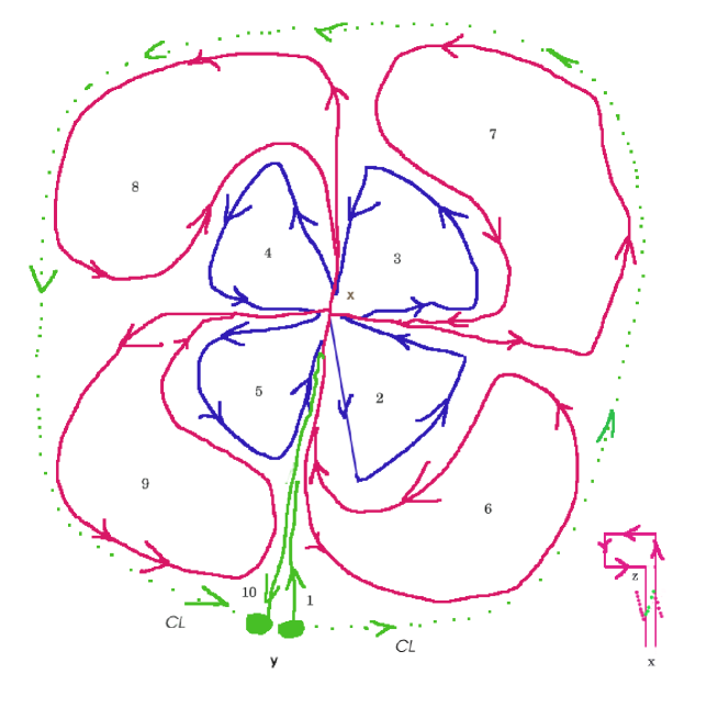
Figure 7: The surface coil-wiring ordering surface integration. Both number of coils and number of wirings, here 4 and 2, are to be increased, refining the surface covering.

The ordering $P_{\ 2}^{\ \Omega}$ for the segmnents at fixed distance from the base point $x$ converges to a flagpole path, shown in the lower right corner of figure 7 .

This path , denoted $\natural$ , starts and ends at the base point $x$ and turns around the plaquette at the point $z$ on the surface ${\cal{S}}$ .

Its contribution inside the ordering $P_{\ 2}^{\ \Omega}$ is

$$\begin{array}[]{l}\natural\ =\ U(\ x\ ,\ z\ ;\ \stackrel{{\scriptstyle{\cal{C}}}}{{\longrightarrow}}\ )\ P_{\ 2}^{\ \Omega\ |\ z}\ \exp\ \left(\ -\ {\displaystyle{\int}}_{\ S_{\ x}}\ {\cal{W}}^{\ (2)}\ \right)\ U\ (\ z\ ,\ x\ ;\ \stackrel{{\scriptstyle{\cal{C}}}}{{\longrightarrow}}\ )\end{array}$$ (141)

The superscript $\Omega$ characterizing the surface ordering $P_{\ 2}^{\ \Omega}$ is chosen to associate a local gauge transformation with the surface ${\cal{S}}$ . This follows from the similarity transformation induced on the flagpole path $\natural$ as defined in eq. (141).

To make this explicit we rename the parallel transport matrix $U\ (\ z\ ,\ x\ ;\ \stackrel{{\scriptstyle{\cal{C}}}}{{\longrightarrow}}\ )$ associated with the fixed base point $x$ and the point $z$ varying over the entire surface ${\cal{S}}$

$$\begin{array}[]{l}U\ (\ z\ ,\ x\ ;\ \stackrel{{\scriptstyle{\cal{C}}}}{{\longrightarrow}}\ )\ \longrightarrow\ \omega_{\ x}\ (\ z\ )\ \rightarrow\vspace*{0.3cm}\\ \natural\ =\ \left(\ \omega_{\ x}\ (\ z\ )\ \right)^{\ -1}\ P_{\ 2}^{\ \Omega\ |\ z}\ \exp\ \left(\ -\ {\displaystyle{\int}}_{\ S_{\ x}}\ {\cal{W}}^{\ (2)}\ \right)\ \omega_{\ x}\ (\ z\ )\vspace*{0.5cm}\\ \omega_{\ x}\ (\ z\ )\ =\left.\omega_{\ x}\ (\ z\ )\ \right|_{\ {\cal{C}}}\end{array}$$ (142)

The last line in eq. (142) shall make it explicit, that the parallel transport matrices $\omega_{\ x}\ (\ z\ )$ are not local functions of the surface point z. Rather they depend on the path, one each from $x$ to $z$ .

The family of similarity transformations $\left\{\ \omega_{\ x}\ (\ z\ )\ \right\}$ induced on the local field strength differential ${\cal{W}}^{\ (2)}\ =\ {\cal{W}}^{\ (2)}\ (\ z\ )$ reflects the nested structure of the weaving pattern defining $P_{\ 2}^{\ \Omega}$ as a whole .

Looking at the structure of the similarity transformations forming the nonlocal structure $\natural$ in eq. (142) the question arises, whether there exists a local gauge transformation $\widehat{\Omega}$ - adapted to ${\cal{S}}$ - which would render the gauge transformed set $\left\{\ \omega_{\ x}^{\ \widehat{\Omega}}\ (\ z\ )\ \right\}$ trivial

$$\begin{array}[]{l}\left.\omega_{\ x}^{\ \widehat{\Omega}}\ =\ \widehat{\Omega}\ (\ z\ )\ \omega_{\ x}\ \left(\ \widehat{\Omega}\ (\ x\ )\ \right)^{\ -1}\ \right|_{\ {\cal{C}}}\ =\ \P\hskip 8.5359pt,\hskip 8.5359pt\forall\ z\ \in\ {\cal{S\vspace*{0.3cm}}}\\ \widehat{\Omega}\ \rightarrow\ \mbox{Riemann normal gauge}\end{array}$$ (143)

Indeed the gauge transformation with the requirements in eq. (143) exists and can be found together with a coordinate transformation of local coordinates on ${\cal{S}}$ and the original contour ${\cal{CL}}$ such that ${\cal{S}}$ becomes the inner part of a bounding circle. The latter forms in the new coordinates the closed contour ${\cal{CL}}$ and the family of curves from the base point $x$ to $z$ becomes the family of straight radial lines. The point $y$ punctuating the contour ${\cal{CL}}$ then can be mapped on the south pole of the bounding circle ( to be definite ) .

The transformed variables are well known in the analogous situation, where gauge transformations refer to coordinate transformations, i.e. the tangent space (universal) spin bundle. The respective coordinates are called Riemann normal coordinates. The gauge equivalent we shall call the Riemann normal gauge as indicated in eq. (143) .

The Riemann normal gauge is also known as radial gauge, at least in the case of an abelian gauge group.

It is precisely in the Riemann normal gauge where the $P_{\ 2}^{\ \Omega}\ \rightarrow\ P_{\ 2}^{\ \widehat{\Omega}}$ ordering becomes ’normal’ . Transforming to the Riemann normal gauge $R.n.g.\ (\ {\cal{S}}\ )$ we have

$$\begin{array}[]{l}R.n.g.\ (\ {\cal{S}}\ )\ :\vspace*{0.3cm}\\ \begin{array}[]{ccl}\left.\omega_{\ x}\ (\ z\ )\ \right|_{\ {\cal{C}}}&\rightarrow&\left.\ \omega_{\ x}^{\ \widehat{\Omega}}\ (\ z\ )\ \right|_{\ {\cal{C}}}\ \equiv\ \P\vspace*{0.3cm}\\ P_{\ 2}^{\ \Omega}&\rightarrow&P_{\ 2}^{\ \widehat{\Omega}}\vspace*{0.3cm}\\ {\cal{W}}^{\ (2)}\ (\ z\ )&\rightarrow&{\cal{W}}^{\ (2)\ \widehat{\Omega}}\ (\ z\ )\ =\ \widehat{\Omega}\ (\ z\ )\ {\cal{W}}^{\ (2)}\ (\ z\ )\ \left(\ \widehat{\Omega}\ (\ z\ )\ \right)^{\ -1}\end{array}\end{array}$$ (144)

Using the transformad quantities on the right hand side of eq. (144) we undo first the flagpole sequence $\natural$ in eq. (142)

$$\begin{array}[]{l}\natural\ =\ \left(\ \omega_{\ x}\ (\ z\ )\ \right)^{\ -1}\ P_{\ 2}^{\ \Omega\ |\ z}\ \exp\ \left(\ -\ {\displaystyle{\int}}_{\ S_{\ x}}\ {\cal{W}}^{\ (2)}\ \right)\ \omega_{\ x}\ (\ z\ )\ \rightarrow\ \natural^{\ \widehat{\Omega}}\vspace*{0.3cm}\\ \natural^{\ \widehat{\Omega}}\ =\ P_{\ 2}^{\ \widehat{\Omega}\ |\ z}\ \exp\ \left(\ -\ {\displaystyle{\int}}_{\ S_{\ x}}\ {\cal{W}}^{\ (2)\ \widehat{\Omega}}\ \right)\end{array}$$ (145)

Next eq. (140) becomes

$$\begin{array}[]{l}U^{\ \widehat{\Omega}}\ \left(\ y\ ,\ y\ ;\ {\cal{CL}}\hskip 14.22636pt\begin{array}[]{c}\longleftarrow\vspace*{-0.42cm}\\ \swarrow\hskip 14.22636pt\nearrow\vspace*{-0.43cm}\\ \longrightarrow\end{array}\right)_{\ A\ B}\ =\vspace*{0.3cm}\\ \hskip 8.5359pt=\ \left(\ P_{\ 2}^{\ \widehat{\Omega}}\ \exp\ \left(\ -\ {\displaystyle{\int}}_{\ S_{\ x}}\ {\cal{W}}^{\ (2)\ \widehat{\Omega}}\ \right)\ \right)_{\ A\ B}\vspace*{0.3cm}\\ \hline\cr\vspace*{-0.2cm}\\ \ \left(\ U_{\ (2)}\ (\ x\ ;\ P_{\ 2}^{\ \widehat{\Omega}}\ |\ {\cal{CL}}\ =\ \partial\ S\ )\ \right)_{\ A\ B}\hskip 11.38092pt\rightarrow\ U_{\ (2)}^{\ \widehat{\Omega}}\ (\ x\ ;\ {\cal{CL}}\ =\ \partial\ S\ )\vspace*{0.3cm}\\ \hskip 71.13188pt=\ \left(\ P_{\ 2}^{\ \widehat{\Omega}}\ \exp\ \left(\ -\ {\displaystyle{\int}}_{\ S_{\ x}}\ {\cal{W}}^{\ (2)\ \widehat{\Omega}}\ \right)\ \right)_{\ A\ B}\end{array}$$ (146)

At this stage, although implicit in the original definition of the general $P_{\ 2}^{\ \Omega}$ ordering, it remains to indicate the (or a) simplified ordering in the Riemann normal gauge. This is shown in figure 8 .

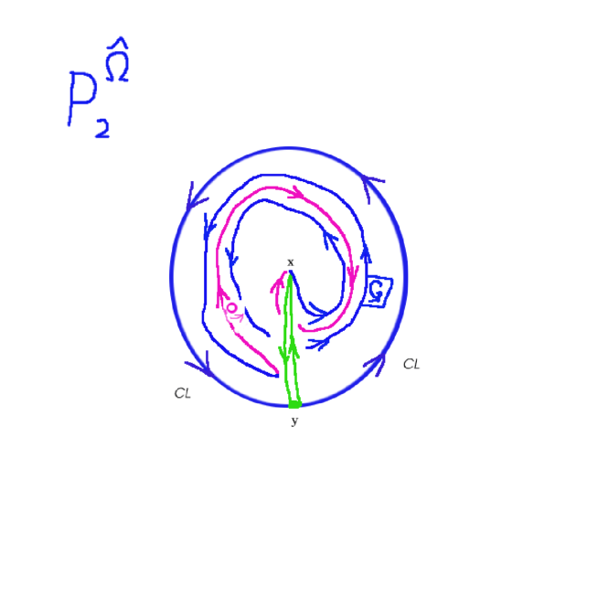
Figure 8: The abridged ordering of plaquettes in the Riemann normal gauge. It follows a double spiral pattern from the base point $x$ and back.

In the Riemann normal gauge the repeated intermediate returns to the base point $x$ are no more necessary .

An interesting shortcut is shown in an actual spiderweb in figure 9.

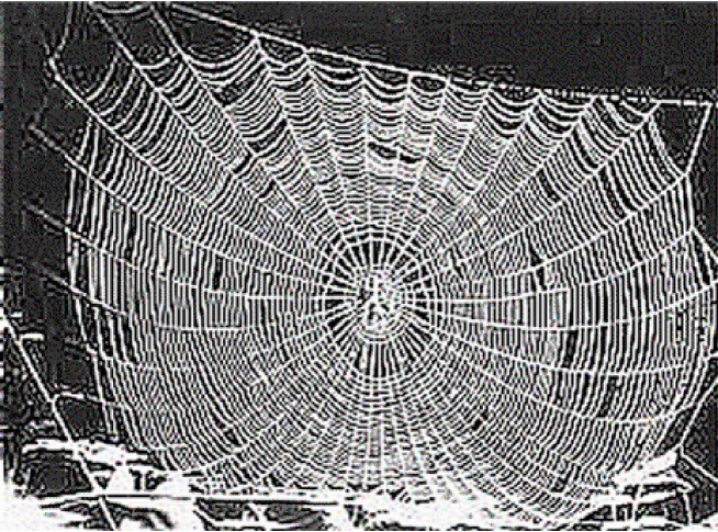
Figure 9: The abridged ordering in an actual spider web. It follows an abridged double spiral pattern from the base point $x$ and back. The figure is adapted from a photograph [39] .

Several remarks conclude this discussion :

i) back to the original gauge

In eq. (146) we have to transform back from Riemann normal gauge on the surface ${\cal{S}}_{\ x\ |\ y}$ to the original gauge

$$\begin{array}[]{l}U\ \left(\ y\ ,\ y\ ;\ {\cal{CL}}\hskip 14.22636pt\begin{array}[]{c}\longleftarrow\vspace*{-0.42cm}\\ \swarrow\hskip 14.22636pt\nearrow\vspace*{-0.43cm}\\ \longrightarrow\end{array}\right)_{\ A\ B}\ =\vspace*{0.3cm}\\ \hskip 8.5359pt=\ \left(\ \left(\ \widehat{\Omega}\ (\ y\ )\ \right)^{\ -1}\ U^{\ \widehat{\Omega}}\ \left(\ y\ ,\ y\ ;\ {\cal{CL}}\hskip 14.22636pt\begin{array}[]{c}\longleftarrow\vspace*{-0.42cm}\\ \swarrow\hskip 14.22636pt\nearrow\vspace*{-0.43cm}\\ \longrightarrow\end{array}\ \right)\ \widehat{\Omega}\ (\ y\ )\ \right)_{\ A\ B}\vspace*{0.1cm}\end{array}$$ (147)

ii) cut the edges of the contour ${\cal{CL}}$

In order to transform the map of the contour ${\cal{CL}}$ continuously into a circle, the edges marked in the corresponding symbol in eqs. (127), (140), (146) and (147) need to be cut

$$\begin{array}[]{l}\begin{array}[]{c}\longleftarrow\vspace*{-0.42cm}\\ \swarrow\hskip 14.22636pt\nearrow\vspace*{-0.43cm}\\ \longrightarrow\end{array}\ \rightarrow\ \hskip 1.42271pt\bigcirc\vspace*{0.1cm}{\scriptstyle{\wedge}}\end{array}$$ (148)

iii) the full collection of surfaces and Riemann normal gauges

As indicated in point i) the meaning of Stokes relations summarized in eqs. (146) and (147) is to consider all surfaces with boundary ${\cal{CL}}\ (\ y\ )$, the latter punctuated at the point $y$, the former with base point $x$, inheriting the point $y$, and the associated Riemann normal gauges $\widehat{\Omega}\ (\ x\ )$ .

The collection of surfaces and associated Riemann normal gauges shall be denoted

$$\begin{array}[]{l}\left\{\ {\cal{S}}_{\ x\ |\ y}\ ;\ \widehat{\Omega}\ (\ x\ )\ \right\}\end{array}$$ (149)

iv) the Stokes relations proper

Stokes relations in eq. (146) in Riemann normal gauges take the form

$$\begin{array}[]{l}U^{\ \widehat{\Omega}_{\ x}}\ \left(\ y\ ,\ y\ ;\ {\cal{CL}}\ (\ y\ )\hskip 5.69046pt\begin{array}[]{l}\hskip 1.42271pt\bigcirc\vspace*{0.1cm}{\scriptstyle{\wedge}}\end{array}\ \right)_{\ A\ B}\ =\vspace*{0.3cm}\\ \hskip 8.5359pt=\ \left(\ P_{\ 2}^{\ \widehat{\Omega}_{\ x}}\ \exp\ \left(\ -\ {\displaystyle{\int}}_{\ S_{\ x\ |\ y}}\ {\cal{W}}^{\ (2)\ \widehat{\Omega}_{\ x}}\ \right)\ \right)_{\ A\ B}\vspace*{0.3cm}\\ \hskip 8.5359pt\forall\hskip 8.5359pt\left\{\ {\cal{S}}_{\ x\ |\ y}\ ;\ \widehat{\Omega}_{\ x}\ \right\}\end{array}$$ (150)

The true form of Stokes relations returns to a general common gauge, combining eqs. (147) and (150)

$$\begin{array}[]{l}U\ \left(\ y\ ,\ y\ ;\ {\cal{CL}}\ (\ y\ )\hskip 5.69046pt\begin{array}[]{l}\hskip 1.42271pt\bigcirc\vspace*{0.1cm}{\scriptstyle{\wedge}}\end{array}\ \right)_{\ A\ B}\ =\vspace*{0.3cm}\\ \hskip 8.5359pt=\ \left(\begin{array}[]{l}\ \left(\ \widehat{\Omega}_{\ x}\ (\ y\ )\ \right)^{\ -1}\ \times\vspace*{0.3cm}\\ \hskip 42.67912pt\times\ P_{\ 2}^{\ \widehat{\Omega}_{\ x}}\ \exp\ \left(\ -\ {\displaystyle{\int}}_{\ S_{\ x\ |\ y}}\ {\cal{W}}^{\ (2)\ \widehat{\Omega}_{\ x}}\ \right)\ \times\vspace*{0.3cm}\\ \hskip 99.58464pt\times\ \widehat{\Omega}_{\ x}\ (\ y\ )\end{array}\ \right)_{\ A\ B}\vspace*{0.7cm}\\ \hskip 8.5359pt\forall\hskip 8.5359pt\left\{\ {\cal{S}}_{\ x\ |\ y}\ ;\ \widehat{\Omega}_{\ x}\ \right\}\end{array}$$ (151)

The closed contour ${\cal{CL}}\ (\ y\ )$ integral $U\ \left(\ y\ ,\ y\ ;\ {\cal{CL}}\ (\ y\ )\hskip 5.69046pt\begin{array}[]{l}\hskip 1.42271pt\bigcirc\vspace*{0.1cm}{\scriptstyle{\wedge}}\end{array}\ \right)$ on the left hand side of eq. (151) is dependent on the point $y$, where the contour begins and ends, but not on any surface and associated Riemann normal gauge forming the collection $\left\{\ {\cal{S}}_{\ x\ |\ y}\ ;\ \widehat{\Omega}_{\ x}\ \right\}$ .

v) the surface integral proper in Riemann normal gauge

The main ingredient in the Stokes relations in eq. (151) is
– selecting a surface and a Riemann normal gauge
out of the collection $\left\{\ {\cal{S}}_{\ x\ |\ y}\ ;\ \widehat{\Omega}_{\ x}\ \right\}$ – the surface integral proper as summarized in eq. (150)

$$\begin{array}[]{l}U^{\ \widehat{\Omega}_{\ x}}\ \left(\ y\ ,\ y\ ;\ {\cal{CL}}\ (\ y\ )\hskip 5.69046pt\begin{array}[]{l}\hskip 1.42271pt\bigcirc\vspace*{0.1cm}{\scriptstyle{\wedge}}\end{array}\ \right)_{\ A\ B}\ =\vspace*{0.3cm}\\ \hskip 8.5359pt=\ \left(\ P_{\ 2}^{\ \widehat{\Omega}_{\ x}}\ \exp\ \left(\ -\ {\displaystyle{\int}}_{\ S_{\ x\ |\ y}}\ {\cal{W}}^{\ (2)\ \widehat{\Omega}_{\ x}}\ \right)\ \right)_{\ A\ B}\end{array}$$ (152)

The surface integral on the right hand side of eq. (152) – in Riemann normal gauge – involves the ordering, denoted $P_{\ 2}^{\ \widehat{\Omega}_{\ x}}$ , of products of local surface differentials ${\cal{W}}^{\ (2)\ \widehat{\Omega}_{\ x}}$ . By this local property the surface ’integral’ is indeed an integral.

In any gauge other than a Riemannian normal one, the corresponding differentials are not local functions of the plaquette differentials, rather they depend on the entire set of flagpole paths, described in figure 7 and eqs. (141) and (142).

vi) the ordering of surface elements in Riemann normal gauge

The path ordering $P_{\ 2}^{\ \widehat{\Omega}_{\ x}}$ of the – matrix valued – surface elements is very special to Riemann normal gauges.

It derives from two steps, starting in a general (original) gauge.

They are described in the text following eq.(140) and in figures 7 and 8.

An appropriate name for $P_{\ 2}^{\ \widehat{\Omega}_{\ x}}$ is ’spider-web ordering’ illustrated in figure 9 , [39] .

A.4 Spin projection operations on adjoint string operators

The adjoint string operators forming binary gluonic mesons are interoduced in eq. (14) , repeated below

$$\begin{array}[]{l}B_{\ \left[\ \mu_{1}\ \nu_{1}\ \right]\ ,\ \left[\ \mu_{2}\ \nu_{2}\ \right]}\ (\ x_{\ 1}\ ,\ x_{\ 2}\ )\ =\vspace*{0.3cm}\\ \hskip 14.22636ptF_{\ \left[\ \mu_{1}\ \nu_{1}\ \right]}\ (\ x_{\ 1}\ ;\ A\ )\ U\ (\ x_{\ 1}\ ,\ A\ ;\ x_{\ 2}\ ,\ B\ )\ F_{\ \left[\ \mu_{2}\ \nu_{2}\ \right]}\ (\ x_{\ 2}\ ;\ B\ )\vspace*{0.3cm}\\ A\ ,\ B\ ,\cdots\ =\ 1,\cdots,8\end{array}$$ (153)

The Lorentz invariant tensors $K^{\ \pm}$ are introduced in eq. (23) , repeated below

$$\begin{array}[]{l}\widetilde{t}_{\ \underline{.}\ ;\ I^{\ \pm}}\ (\ z\ ,\ p\ ,\ J^{\ \pm\ +}\ ;\ .\ )\ =\ \left(\begin{array}[]{l}\ \left(\ K^{\ \pm}\ \right)_{\ \ \left[\ \mu_{\ 1}\ \nu_{\ 1}\ \right]\ \left[\ \mu_{\ 2}\ \nu_{\ 2}\ \right]}\ \times\vspace*{0.3cm}\\ \hskip 19.91684pt\times\ \widetilde{t}_{\ I^{\ \pm}}\ (\ z\ ,\ p\ ,\ J^{\ \pm\ +}\ ;\ .\ )\end{array}\ \right)\vspace*{0.5cm}\\ \ \left(\ K^{\ +}\ \right)_{\ \ \left[\ \mu_{\ 1}\ \nu_{\ 1}\ \right]\ \left[\ \mu_{\ 2}\ \nu_{\ 2}\ \right]}\ =\ g_{\ \mu_{\ 1}\ \mu_{\ 2}}\ g_{\ \nu_{\ 1}\ \nu_{\ 2}}\ -\ g_{\ \mu_{\ 1}\ \nu_{\ 2}}\ g_{\ \mu_{\ 2}\ \nu_{\ 1}}\vspace*{0.5cm}\\ \ \left(\ K^{\ -}\ \right)_{\ \ \left[\ \mu_{\ 1}\ \nu_{\ 1}\ \right]\ \left[\ \mu_{\ 2}\ \nu_{\ 2}\ \right]}\ =\ \varepsilon_{\ \mu_{\ 1}\ \mu_{\ 2}\ \nu_{\ 1}\ \nu_{\ 2}}\end{array}$$ (154)

We perform the associated projections

$$\begin{array}[]{l}B_{\ \left[\ \mu_{1}\ \nu_{1}\ \right]\ ,\ \left[\ \mu_{2}\ \nu_{2}\ \right]}\ =\ \left(\ \begin{array}[]{r}K^{\ +}_{\ \left[\ \mu_{1}\ \nu_{1}\ \right]\ \left[\ \mu_{2}\ \nu_{2}\ \right]}\ B^{\ (+)}\ +\vspace*{0.3cm}\\ +\ K^{\ -}_{\ \left[\ \mu_{1}\ \nu_{1}\ \right]\ \left[\ \mu_{2}\ \nu_{2}\ \right]}\ B^{\ (-)}\ +\vspace*{0.3cm}\\ +\ B^{\ {}^{\prime}}_{\ \left[\ \mu_{1}\ \nu_{1}\ \right]\ ,\ \left[\ \mu_{2}\ \nu_{2}\ \right]}\end{array}\ \right)\end{array}$$ (155)

The decomposition according to eq. (155) is the same for the Riemann curvature tensor, where $B^{\ (+)}$ relates to the curvature scalar , $B^{\ {}^{\prime}}$ to the Ricci and Weyl tensors and $B^{\ (-)}\ =\ 0$, unlike here.

So we form the metric (Ricci-) contraction

$$\begin{array}[]{l}g^{\ \mu_{\ 1}\ \mu_{\ 2}}\ B_{\ \left[\ \mu_{1}\ \nu_{1}\ \right]\ ,\ \left[\ \mu_{2}\ \nu_{2}\ \right]}\ =\ R_{\ \nu_{\ 1}\ \nu_{\ 2}}\vspace*{0.3cm}\\ R_{\ \nu_{\ 1}\ \nu_{\ 2}}\ =\ \left(\ \begin{array}[]{l}3\ g_{\ \nu_{\ 1}\ \nu_{\ 2}}\ B^{\ (+)}\ +\vspace*{0.3cm}\\ +\ g^{\ \mu_{\ 1}\ \mu_{\ 2}}\ B^{\ {}^{\prime}}_{\ \left[\ \mu_{1}\ \nu_{1}\ \right]\ ,\ \ \left[\ \mu_{2}\ \nu_{2}\ \right]}\end{array}\ \right)\vspace*{0.3cm}\\ R_{\ \nu_{\ 1}\ \nu_{\ 2}}\ =\ \varrho_{\ \nu_{\ 1}\ \nu_{\ 2}}\ +\ \frac{1}{4}\ g_{\ \nu_{\ 1}\ \nu_{\ 2}}\ R\hskip 8.5359pt;\hskip 8.5359ptR\ =\ g^{\ \nu_{\ 1}\ \nu_{\ 2}}\ R_{\ \nu_{\ 1}\ \nu_{\ 2}}\vspace*{0.3cm}\\ \varrho_{\ \nu_{\ 1}\ \nu_{\ 2}}\ =\ R_{\ \nu_{\ 1}\ \nu_{\ 2}}\ -\ \frac{1}{4}\ g_{\ \nu_{\ 1}\ \nu_{\ 2}}\ R\end{array}$$ (156)

It follows from eq. (156)

$$\begin{array}[]{l}\varrho_{\ \nu_{\ 1}\ \nu_{\ 2}}\ =\ g^{\ \mu_{\ 1}\ \mu_{\ 2}}\ B^{\ {}^{\prime}}_{\ \left[\ \mu_{1}\ \nu_{1}\ \right]\ ,\ \ \left[\ \mu_{2}\ \nu_{2}\ \right]}\ \rightarrow\vspace*{0.3cm}\\ g^{\ \mu_{\ 1}\ \mu_{\ 2}}\ g^{\ \nu_{\ 1}\ \nu_{\ 2}}\ B^{\ {}^{\prime}}_{\ \left[\ \mu_{1}\ \nu_{1}\ \right]\ ,\ \ \left[\ \mu_{2}\ \nu_{2}\ \right]}\ =\ 0\hskip 8.5359pt\rightarrow\hskip 8.5359ptR\ =\ 12\ B^{\ (+)}\end{array}$$ (157)

The quantity $B^{\ {}^{\prime}}$ with the trace condition in eq. (157) forms the irreducible relativistic spin two part $S_{\ 12}^{\ +}\ =\ 2$ as defined in eqs. (21) and (22) in the main text. Here we concentrate on the projection on $B^{\ (\pm)}$ .

From eq. (157) we obtain

$$\begin{array}[]{l}B^{\ (+)}\ (\ x_{\ 1}\ ,\ x_{\ 2}\ )\ =\vspace*{0.3cm}\\ \hskip 17.07182pt=\ \frac{1}{12}\ F_{\ \left[\ \alpha\ \beta\ \right]}\ (\ x_{\ 1}\ ;\ A\ )\ U\ (\ x_{\ 1}\ ,\ A\ ;\ x_{\ 2}\ ,\ B\ )\ F^{\ \left[\ \alpha\ \beta\ \right]}\ (\ x_{\ 2}\ ;\ B\ )\end{array}$$ (158)

The projection on $B^{\ (-)}$ proceeds in a similar way

$$\begin{array}[]{l}\varepsilon^{\ \mu_{\ 1}\ \mu_{\ 2}\ \nu_{\ 1}\ \nu_{\ 2}}\ B_{\ \left[\ \mu_{1}\ \nu_{1}\ \right]\ ,\ \left[\ \mu_{2}\ \nu_{2}\ \right]}\ =\ -\ 24\ B^{\ (-)}\ +\vspace*{0.3cm}\\ \hskip 128.0374pt+\ \varepsilon^{\ \mu_{\ 1}\ \mu_{\ 2}\ \nu_{\ 1}\ \nu_{\ 2}}\ B^{\ {}^{\prime}}_{\ \left[\ \mu_{1}\ \nu_{1}\ \right]\ ,\ \ \left[\ \mu_{2}\ \nu_{2}\ \right]}\ \rightarrow\vspace*{0.3cm}\\ \varepsilon^{\ \mu_{\ 1}\ \mu_{\ 2}\ \nu_{\ 1}\ \nu_{\ 2}}\ B^{\ {}^{\prime}}_{\ \left[\ \mu_{1}\ \nu_{1}\ \right]\ ,\ \ \left[\ \mu_{2}\ \nu_{2}\ \right]}\ =\ 0\end{array}$$ (159)

The structure pf $B^{\ (-)}$ follows similarly as for $B^{\ (+)}$ in eq. (158) . We thus give both expressions together below

$$\begin{array}[]{l}B^{\ (+)}\ (\ x_{\ 1}\ ,\ x_{\ 2}\ )\ =\vspace*{0.3cm}\\ \hskip 17.07182pt=\ \frac{1}{12}\ F_{\ \left[\ \alpha\ \beta\ \right]}\ (\ x_{\ 1}\ ;\ A\ )\ U\ (\ x_{\ 1}\ ,\ A\ ;\ x_{\ 2}\ ,\ B\ )\ F^{\ \left[\ \alpha\ \beta\ \right]}\ (\ x_{\ 2}\ ;\ B\ )\vspace*{0.3cm}\\ \hline\cr\vspace*{-0.2cm}\\ B^{\ (-)}\ (\ x_{\ 1}\ ,\ x_{\ 2}\ )\ =\vspace*{0.3cm}\\ \hskip 17.07182pt=\ -\ \frac{1}{12}\ F_{\ \left[\ \alpha\ \beta\ \right]}\ (\ x_{\ 1}\ ;\ A\ )\ U\ (\ x_{\ 1}\ ,\ A\ ;\ x_{\ 2}\ ,\ B\ )\ \widetilde{F}^{\ \left[\ \alpha\ \beta\ \right]}\ (\ x_{\ 2}\ ;\ B\ )\vspace*{0.3cm}\\ \hskip 17.07182pt=\ -\ \frac{1}{12}\ \widetilde{F}_{\ \left[\ \alpha\ \beta\ \right]}\ (\ x_{\ 1}\ ;\ A\ )\ U\ (\ x_{\ 1}\ ,\ A\ ;\ x_{\ 2}\ ,\ B\ )\ F^{\ \left[\ \alpha\ \beta\ \right]}\ (\ x_{\ 2}\ ;\ B\ )\vspace*{0.3cm}\\ \hline\cr\vspace*{-0.2cm}\\ \widetilde{F}_{\ \left[\ \alpha\ \beta\ \right]}\ (\ x_{\ 2}\ ;\ B\ )\ =\ \frac{1}{2}\ \varepsilon_{\ \alpha\ \beta\ \gamma\ \delta}\ F^{\ \left[\ \gamma\ \delta\ \right]}\ (\ x_{\ 2}\ ;\ B\ )\vspace*{0.3cm}\\ \mbox{and}\hskip 8.5359pt(\ x_{\ 2}\ ;\ B\ )\ \leftrightarrow\ (\ x_{\ 1}\ ;\ A\ )\end{array}$$ (160)

A.5 Spin projection operations on adjoint string operators - extended

We continue the projection operations carried out in appendix A.4 in order to extend them to the remaining gb spectral series of type $II^{\ +}$ . This is related to the quantities $B^{\ {}^{\prime}}_{\ \left[\ \mu_{1}\ \nu_{1}\ \right]\ ,\ \left[\ \mu_{2}\ \nu_{2}\ \right]}$ defined in eq. (24) and refined in appendix A.4 ( eq. (155) ) .

To that end we perform the full decomposition of the tensorial structure of the octet string operators interoduced in eq. (14) and rewritten in eq. (153)

$$\begin{array}[]{l}B_{\ \left[\ \mu_{1}\ \nu_{1}\ \right]\ ,\ \left[\ \mu_{2}\ \nu_{2}\ \right]}\ (\ x_{\ 1}\ ,\ x_{\ 2}\ )\ \rightarrow\ B_{\ \left[\ \mu_{1}\ \nu_{1}\ \right]\ ,\ \left[\ \mu_{2}\ \nu_{2}\ \right]}\end{array}$$ (161)

which is analogous to that of the Riemann curvature tensor, without the metric constraints of the latter.

The Ricci contraction introduced in eq. (156) yields the follwoing structure

$$\begin{array}[]{l}B_{\ \left[\ \mu_{1}\ \nu_{1}\ \right]\ ,\ \left[\ \mu_{2}\ \nu_{2}\ \right]}\ =\ w_{\ \left[\ \mu_{1}\ \nu_{1}\ \right]\ \left[\ \mu_{2}\ \nu_{2}\ \right]}+\Delta\ B_{\ \left[\ \mu_{1}\ \nu_{1}\ \right]\ ,\ \left[\ \mu_{2}\ \nu_{2}\ \right]}\vspace*{0.3cm}\\ \Delta\ B_{\ \left[\ \mu_{1}\ \nu_{1}\ \right]\ ,\ \left[\ \mu_{2}\ \nu_{2}\ \right]}\ =\begin{array}[]{l}\ \frac{1}{2}\left(\begin{array}[]{l}g_{\ \mu_{\ 1}\ \mu_{\ 2}}\ R_{\ \nu_{\ 1}\ \nu_{\ 2}}-\ g_{\ \nu_{\ 1}\ \mu_{\ 2}}\ R_{\ \mu_{\ 1}\ \nu_{\ 2}}\vspace*{0.3cm}\\ -\ g_{\ \mu_{\ 1}\ \nu_{\ 2}}\ R_{\ \nu_{\ 1}\ \mu_{\ 2}}\ +\ g_{\ \nu_{\ 1}\ \nu_{\ 2}}\ R_{\ \mu_{\ 1}\ \mu_{\ 2}}\end{array}\right)\vspace*{0.3cm}\\ -\ \frac{1}{6}\ K^{\ +}_{\ \left[\ \mu_{1}\ \nu_{1}\ \right]\ \left[\ \mu_{2}\ \nu_{2}\ \right]}\ R\end{array}\vspace*{0.4cm}\\ \hline\cr\vspace*{-0.3cm}\\ \mbox{with :}\hskip 8.5359ptg^{\ \mu_{\ 1}\ \mu_{\ 2}}\ w_{\ \left[\ \mu_{1}\ \nu_{1}\ \right]\ \left[\ \mu_{2}\ \nu_{2}\ \right]}\ =\ 0\vspace*{0.5cm}\\ g^{\ \mu_{\ 1}\ \mu_{\ 2}}\ B_{\ \left[\ \mu_{1}\ \nu_{1}\ \right]\ \ ,\ \left[\ \mu_{2}\ \nu_{2}\ \right]}\ =\ g^{\ \mu_{\ 1}\ \mu_{\ 2}}\ \Delta\ B_{\ \left[\ \mu_{1}\ \nu_{1}\ \right]\ ,\ \left[\ \mu_{2}\ \nu_{2}\ \right]}\ =\ R_{\ \nu_{\ 1}\ \nu_{\ 2}}\vspace*{0.5cm}\\ R\ =\ g^{\ \nu_{\ 1}\ \nu_{\ 2}}\ R_{\ \nu_{\ 1}\ \nu_{\ 2}}\ =\ 12\ B^{\ (+)}\end{array}$$ (162)

Before proceeding lets express the Ricci bilinear in terms of the base octet string operators $B_{\ \left[\ \mu_{1}\ \nu_{1}\ \right]\ ,\ \left[\ \mu_{2}\ \nu_{2}\ \right]}$

$$\begin{array}[]{l}R_{\ \nu_{\ 1}\ \nu_{\ 2}}\ =\vspace*{0.3cm}\\ \hskip 8.5359pt=\ -\ F_{\ \nu_{\ 1}\ \alpha}\ (\ x_{\ 1}\ ;\ A\ )\ U\ (\ x_{\ 1}\ ,\ A\ ;\ x_{\ 2}\ ,\ B\ )\ F^{\ \alpha}_{\hskip 8.5359pt\nu_{\ 2}}\ (\ x_{\ 2}\ ;\ B\ )\end{array}$$ (163)

In order to simplify notation we shall suppress the position arguments and use chromoelectric and -magnetic fields for the field strength tensor.

$$\begin{array}[]{l}-\ R_{\ \nu_{\ 1}\ \nu_{\ 2}}\ =\ \left(\begin{array}[]{cc}\vec{E}^{\ A}\ \vec{E}^{\ D}&\vec{S}^{\ k\ A\ D}\vspace*{0.5cm}\\ \vec{S}^{\ i\ A\ D}&\begin{array}[]{ll}-\ \vec{E}^{\ i\ A}\ \vec{E}^{\ k\ D}-\ \vec{B}^{\ i\ A}\ \vec{B}^{\ k\ D}\vspace*{0.3cm}\\ \ +\ \delta_{\ ik}\ \vec{B}^{\ A}\ \vec{B}^{\ D}\end{array}\end{array}\ \right)\ U_{\ A\ D}\vspace*{0.5cm}\\ R\ =\ 2\ \left(\ \vec{B}^{\ A}\ \vec{B}^{\ D}\ -\ \vec{E}^{\ A}\ \vec{E}^{\ D}\ \right)\ U_{\ A\ D}\hskip 8.5359pt;\hskip 8.5359pt\vec{S}^{\ A\ D}\ =\ \vec{E}^{\ A}\ \wedge\ \vec{B}^{\ D}\vspace*{0.5cm}\\ \vec{E}^{\ i\ A}\ =\ F^{\ 0\ i\ A}\hskip 8.5359pt,\hskip 8.5359pt\vec{B}^{\ i\ A}\ =\ \frac{1}{2}\ \varepsilon_{\ ikl}\ F^{\ k\ l\ A}\end{array}$$ (164)

In eq. (164) we recognize the Maxwell energy momentum like (bilinear) expression, where $\vec{S}^{\ A\ D}$ shall be called the bilinear Poynting vector.

Next we substitute the traceless part of the Ricci bilinear ( eq. (156) ) in eq. (162)

$$\begin{array}[]{l}-\ \varrho^{\ \mu\ \nu}\ =\ -\ R^{\ \mu\ \nu}\ +\ \frac{1}{4}\ g^{\ \mu\ \nu}\ R\ =\ \vartheta_{\ cl}^{\ \mu\ \nu}\ =\vspace*{0.5cm}\\ \hskip 11.38092pt=\ \left(\begin{array}[]{cc}\frac{1}{2}\ \left(\begin{array}[]{l}\vec{E}^{\ A}\ \vec{E}^{\ D}\vspace*{0.3cm}\\ \hskip 8.5359pt+\ \vec{B}^{\ A}\ \vec{B}^{\ D}\end{array}\ \right)&-\ \vec{S}^{\ k\ A\ D}\vspace*{0.5cm}\\ -\ \vec{S}^{\ i\ A\ D}&\begin{array}[]{ll}-\ \vec{E}^{\ i\ A}\ \vec{E}^{\ k\ D}-\ \vec{B}^{\ i\ A}\ \vec{B}^{\ k\ D}\vspace*{0.3cm}\\ \ +\ \frac{1}{2}\ \delta_{\ ik}\ \left(\begin{array}[]{l}\vec{E}^{\ A}\ \vec{E}^{\ D}\vspace*{0.3cm}\\ \hskip 8.5359pt+\ \vec{B}^{\ A}\ \vec{B}^{\ D}\end{array}\ \right)\end{array}\end{array}\ \right)\ U_{\ A\ D}\end{array}$$ (165)

In eq. (165) we recognize the bilinear with the structure of the classical (traceless) Maxwell energy momentum tensor of nonabelian gauge field strengths.

Eq. (162) becomes decomposed into positive parity irreducible parts

$$\begin{array}[]{l}B_{\ \left[\ \mu_{1}\ \nu_{1}\ \right]\ ,\ \left[\ \mu_{2}\ \nu_{2}\ \right]}\ =\ w_{\ \left[\ \mu_{1}\ \nu_{1}\ \right]\ \left[\ \mu_{2}\ \nu_{2}\ \right]}+\Delta\ B_{\ \left[\ \mu_{1}\ \nu_{1}\ \right]\ ,\ \left[\ \mu_{2}\ \nu_{2}\ \right]}\vspace*{0.3cm}\\ \Delta\ B_{\ \left[\ \mu_{1}\ \nu_{1}\ \right]\ ,\ \left[\ \mu_{2}\ \nu_{2}\ \right]}\ =\begin{array}[]{l}\ \frac{1}{2}\left(\begin{array}[]{l}g_{\ \mu_{\ 1}\ \mu_{\ 2}}\ \varrho_{\ \nu_{\ 1}\ \nu_{\ 2}}-\ g_{\ \nu_{\ 1}\ \mu_{\ 2}}\ \varrho_{\ \mu_{\ 1}\ \nu_{\ 2}}\vspace*{0.3cm}\\ -\ g_{\ \mu_{\ 1}\ \nu_{\ 2}}\ \varrho_{\ \nu_{\ 1}\ \mu_{\ 2}}\ +\ g_{\ \nu_{\ 1}\ \nu_{\ 2}}\ \varrho_{\ \mu_{\ 1}\ \mu_{\ 2}}\end{array}\right)\vspace*{0.3cm}\\ +\ \frac{1}{12}\ K^{\ +}_{\ \left[\ \mu_{1}\ \nu_{1}\ \right]\ \left[\ \mu_{2}\ \nu_{2}\ \right]}\ R\end{array}\vspace*{0.4cm}\\ \hline\cr\vspace*{-0.3cm}\\ \mbox{with :}\hskip 8.5359ptg^{\ \mu_{\ 1}\ \mu_{\ 2}}\ w_{\ \left[\ \mu_{1}\ \nu_{1}\ \right]\ \left[\ \mu_{2}\ \nu_{2}\ \right]}\ =\ 0\vspace*{0.5cm}\\ g^{\ \mu_{\ 1}\ \mu_{\ 2}}\ B_{\ \left[\ \mu_{1}\ \nu_{1}\ \right]\ \ ,\ \left[\ \mu_{2}\ \nu_{2}\ \right]}\ =\ g^{\ \mu_{\ 1}\ \mu_{\ 2}}\ \Delta\ B_{\ \left[\ \mu_{1}\ \nu_{1}\ \right]\ ,\ \left[\ \mu_{2}\ \nu_{2}\ \right]}\ =\ R_{\ \nu_{\ 1}\ \nu_{\ 2}}\vspace*{0.5cm}\\ R\ =\ g^{\ \nu_{\ 1}\ \nu_{\ 2}}\ R_{\ \nu_{\ 1}\ \nu_{\ 2}}\ =\ 12\ B^{\ (+)}\end{array}$$ (166)

As a side remark to the (Lorentz-) tensorial reduction of the bilinear quantities $B_{\ \left[\ \mu_{1}\ \nu_{1}\ \right]\ ,\ \left[\ \mu_{2}\ \nu_{2}\ \right]}$ it is necessary to include the spatio-temporal nonlocal parallel transport matrices pertaining to a general connection and metric $\Gamma^{\hskip 8.5359pt\mu}_{\ \sigma\hskip 8.5359pt\nu}$ and $g_{\ \mu\nu}$ . This is necessary to render $B_{\ \left[\ \mu_{1}\ \nu_{1}\ \right]\ ,\ \left[\ \mu_{2}\ \nu_{2}\ \right]}$ a true nonlocal Lorentz-tensor. We do not do this here. In globally flat Minkowski space coordinates this parallel transport is trivial.

The sequence of projections on first Lorentz spin ($\underline{.}$) and second on rotational spin (.) , needs two steps , rearranging the structure of $-\ \varrho^{\ \mu\nu}$ in eq. (165)

$$\begin{array}[]{l}-\ \varrho^{\ \mu\ \nu}\ =\ \vartheta_{\ cl}^{\ \mu\ \nu}\ =\vspace*{0.5cm}\\ \hskip 2.84544pt=\left(\begin{array}[]{cc}\frac{1}{2}\ \left(\begin{array}[]{l}\vec{E}^{\ A}\ \vec{E}^{\ D}\vspace*{0.3cm}\\ \hskip 8.5359pt+\ \vec{B}^{\ A}\ \vec{B}^{\ D}\end{array}\ \right)&-\ \vec{S}^{\ k\ A\ D}\vspace*{0.5cm}\\ -\ \vec{S}^{\ i\ A\ D}&\begin{array}[]{ll}\left(\begin{array}[]{l}-\ \vec{E}^{\ i\ A}\ \vec{E}^{\ k\ D}-\ \vec{B}^{\ i\ A}\ \vec{B}^{\ k\ D}\vspace*{0.3cm}\\ +\ \frac{1}{3}\ \delta_{\ ik}\ \left(\begin{array}[]{l}\vec{E}^{\ A}\ \vec{E}^{\ D}\vspace*{0.3cm}\\ \hskip 8.5359pt+\ \vec{B}^{\ A}\ \vec{B}^{\ D}\end{array}\ \right)\end{array}\ \right)\vspace*{0.6cm}\\ +\ \frac{1}{6}\ \delta_{\ ik}\ \left(\begin{array}[]{l}\vec{E}^{\ A}\ \vec{E}^{\ D}\vspace*{0.3cm}\\ \hskip 8.5359pt+\ \vec{B}^{\ A}\ \vec{B}^{\ D}\end{array}\ \right)\end{array}\end{array}\right)\ \times\vspace*{0.3cm}\\ \hskip 159.3356pt\times\ U_{\ A\ D}\end{array}$$ (167)

The tensor structure of $\vartheta_{\ cl}^{\ \mu\ \nu}$ in eq. (167) follows the hydrodynamic nomenclature

$$\begin{array}[]{l}-\ \varrho^{\ \mu\ \nu}\ =\ \vartheta_{\ cl}^{\ \mu\ \nu}\ =\ \left(\begin{array}[]{cc}\varrho_{\ e}&-\ \vec{S}^{\ k}\vspace*{0.5cm}\\ -\ \vec{S}^{\ i}&\left(\ \begin{array}[]{cc}\pi_{\ i\ k}\vspace*{0.3cm}\\ +\ \delta_{\ ik}\ p\end{array}\ \right)\end{array}\right)\vspace*{0.3cm}\\ \varrho_{\ e}\ =\ 3\ p\ =\ \frac{1}{2}\ \left(\ \vec{E}^{\ A}\ \vec{E}^{\ D}\ +\ \vec{B}^{\ A}\ \vec{B}^{\ D}\ \right)\ U_{\ A\ D}\vspace*{0.3cm}\\ \pi_{\ i\ k}\ =\ 2\ p\ \delta_{\ i\ k}\ -\ \left(\ \vec{E}^{\ i\ A}\ \vec{E}^{\ k\ D}\ +\ \vec{B}^{\ i\ A}\ \vec{B}^{\ k\ D}\ \right)\ U_{\ A\ D}\vspace*{0.3cm}\\ \sum_{\ i}\ \pi_{\ i\ i}\ =\ 0\end{array}$$ (168)

with the identifications given in eq. (168) .

The chain of irreducible components of $\Delta\ B_{\ \underline{.}}$ is shown in eq. (169) below

$$\begin{array}[]{l}\begin{array}[]{|c|cc cc|}\hline\cr&&&&\vspace*{-0.3cm}\hfil\\ \mbox{step}&\mbox{name}&\mbox{\# comp.}&\mbox{L.-spin}&\mbox{R.-spin}\\ &&&&\vspace*{-0.3cm}\hfil\\ \hline\cr&&&&\vspace*{-0.3cm}\hfil\\ 1&\Delta\ B_{\ \underline{.}}&10&\mbox{mixed}&\mbox{mixed}\\ 2&B^{\ (+)}&1&1&1\\ 2&\varrho^{\ \underline{.}}&9&D^{\ 1\ ,\ \overline{1}}&\mbox{mixed}\\ 3&\varrho_{\ e}&1&-&1\\ 3&\vec{S}&3&-&D^{\ 1}\\ 3&\pi_{\ .}&5&-&D^{\ 2}\vspace*{-0.3cm}\\ &&&&\\ \hline\cr\end{array}\end{array}$$ (169)

It is the last term in eq. (169) $\pi_{\ i\ k}$ as displayed in eq. (168) which characterizes the $S_{\ 12}^{\ +}\ =\ 2$ spectral series of binary gluonic mesons. The R-spin 2 tensor $\pi_{\ i\ k}$ is related to the corresponding components of the Weyl bilinear $w_{\ \left[\ \mu_{1}\ \nu_{1}\ \right]\ \left[\ \mu_{2}\ \nu_{2}\ \right]}$ introduced in eq. (162), which represents the traceless part of the bilinear Riemann like tensor $B_{\ \left[\ \mu_{1}\ \nu_{1}\ \right]\ ,\ \left[\ \mu_{2}\ \nu_{2}\ \right]}$ , to which we turn next.

Weyl bilinear and circular polarization basis for gauge field strengths

We recall the right and left chiral spin matrices defined in appendix A.1 ( eqs. (62) and (63) ) reproduced below, first for the right circular part. Here the notion right (left) circular refers to a fixed spin axis and not to the individual momenta of the two gauge bosons at the end of the octet string, in question. The spin axis is common to both and an axial vector.

$$\begin{array}[]{l}\left(\ \sigma_{\ \mu\ \nu}\ \right)_{\ \alpha}^{\hskip 8.5359pt\beta}\ \leftrightarrow\ P_{\ R}\ \frac{i}{2}\ \left[\ \gamma_{\ \mu}\ ,\ \gamma_{\ \nu}\ \right]\ P_{\ R}\hskip 8.5359pt;\hskip 8.5359ptP_{\ R}\ =\ \frac{1}{2}\ (\ 1\ +\ \gamma_{\ 5\ R}\ )\vspace*{0.3cm}\\ \gamma_{\ 5\ R}\ =\ \frac{1}{i}\ \gamma_{\ 0}\ \gamma_{\ 1}\ \gamma_{\ 2}\ \gamma_{\ 3}\vspace*{0.3cm}\\ \left(\ \sigma_{\ \mu\ \nu}\ \right)_{\ \alpha}^{\hskip 8.5359pt\beta}\ =\ \begin{array}[]{ll}\ \left(\begin{array}[]{l}-\ i\ \Sigma_{\ k}\vspace*{0.3cm}\\ \varepsilon_{\ mnr}\ \Sigma_{\ r}\end{array}\ \right)_{\alpha}^{\hskip 8.5359pt\beta}\vspace*{1.0cm}&\vspace*{-0.5cm}\begin{array}[]{l}\mbox{for}\ \mu\ =\ 0\ ,\ \nu\ =\ k\ =\ 1,2,3\vspace*{0.3cm}\\ \mbox{for}\ \mu\ =\ m\ ,\ \nu\ =\ n\ ;\vspace*{-0.2cm}\\ \hskip 76.82234ptm,n,r\ =\ 1,2,3\end{array}\end{array}\vspace*{0.3cm}\\ \left(\ \sigma_{\ \mu\ \nu}\ \right)_{\ \alpha}^{\hskip 8.5359pt\beta}\ \rightarrow\ \sigma_{\ \mu\ \nu}^{\ R}\hskip 8.5359pt;\hskip 8.5359pt\sigma_{\ \mu\ \nu}^{\ R}\ =\ -\ i\ \frac{1}{2}\ \varepsilon_{\ \mu\nu\varrho\tau}\ \sigma^{\ \varrho\ \tau\ R}\end{array}$$ (170)

The right circular spinor basis in eq. (170) yields the projection on the gauge field strengths

$$\begin{array}[]{l}\frac{1}{2}\ \sigma_{\ \mu\ \nu}^{\ R}\ F^{\ \left[\ \mu\ \nu\ \right]}\ (\ x\ ;\ A\ )\ =\ \Sigma_{\ r}\ \vec{C}^{\ r\ A}\ (\ x\ )\vspace*{0.3cm}\\ \vec{C}^{\ r\ A}\ (\ x\ )\ =\ \left(\ \vec{B}\ -\ i\ \vec{E}\ \right)^{\ r\ A}\ (\ x\ )\hskip 8.5359pt\rightarrow\hskip 8.5359pt\vec{C}^{\ r\ A}\vspace*{0.3cm}\\ r\ =\ 1,2,3\end{array}$$ (171)

The right circular quantities $\vec{C}^{\ A}$ in eq. (171) are complex combinations of the hermitian field strengths $F^{\ \left[\ \mu\ \nu\ \right]\ A}$ in the adjoint representation of $SU3_{\ c}$ .

We note the right circular identity, following from eq. (170)

$$\begin{array}[]{l}\frac{1}{2}\ \sigma_{\ \mu\ \nu}^{\ R}\ F^{\ \left[\ \mu\ \nu\ \right]\ A}\ \equiv\ \frac{1}{2}\ \sigma_{\ \mu\ \nu}^{\ R}\ \left(\ F^{\ R}\ \right)^{\ \left[\ \mu\ \nu\ \right]\ A}\vspace*{0.3cm}\\ \ \left(\ F^{\ R}\ \right)^{\ \left[\ \mu\ \nu\ \right]\ A}\ =\ \frac{1}{2}\ \left(\ F^{\ \left[\ \mu\ \nu\ \right]\ A}\ -\ i\ \widetilde{F}^{\ \left[\ \mu\ \nu\ \right]\ A}\ \right)\vspace*{0.3cm}\\ \widetilde{F}_{\ \left[\ \mu\ \nu\ \right]}^{\ A}\ =\ \frac{1}{2}\ \varepsilon_{\ \mu\nu\sigma\tau}\ F^{\ \left[\ \sigma\ \tau\ \right]\ A}\end{array}$$ (172)

When the space-time component $r$ in $\vec{C}^{\ r\ A}$ is explicitely denoted, the vector symbol of $\vec{C}$ shall be omitted for simplicity.

Now we recall the left chiral spinor matrices defined in eqs. (81) and (82) in appendix A.1

$$\begin{array}[]{l}\left(\ \sigma_{\ \mu\ \nu}\ \right)^{\ \dot{\gamma}}_{\hskip 11.38092pt\dot{\delta}}\ \leftrightarrow\ P_{\ L}\ \frac{i}{2}\ \left[\ \gamma_{\ \mu}\ ,\ \gamma_{\ \nu}\ \right]\ P_{\ L}\hskip 8.5359pt;\hskip 8.5359ptP_{\ L}\ =\ \frac{1}{2}\ (\ 1\ -\ \gamma_{\ 5\ R}\ )\vspace*{0.3cm}\\ \gamma_{\ 5\ R}\ =\ \frac{1}{i}\ \gamma_{\ 0}\ \gamma_{\ 1}\ \gamma_{\ 2}\ \gamma_{\ 3}\vspace*{0.3cm}\\ \left(\ \sigma_{\ \mu\ \nu}\ \right)^{\ \dot{\gamma}}_{\hskip 11.38092pt\dot{\delta}}\ =\ \begin{array}[]{ll}\ \left(\begin{array}[]{l}i\ \Sigma_{\ k}\vspace*{0.3cm}\\ \varepsilon_{\ mnr}\ \Sigma_{\ r}\end{array}\ \right)^{\dot{\gamma}}_{\hskip 11.38092pt\dot{\delta}}\vspace*{1.0cm}&\vspace*{-0.5cm}\begin{array}[]{l}\mbox{for}\ \mu\ =\ 0\ ,\ \nu\ =\ k\ =\ 1,2,3\vspace*{0.3cm}\\ \mbox{for}\ \mu\ =\ m\ ,\ \nu\ =\ n\ ;\vspace*{-0.2cm}\\ \hskip 76.82234ptm,n,r\ =\ 1,2,3\end{array}\end{array}\vspace*{0.3cm}\\ \left(\ \sigma_{\ \mu\ \nu}\ \right)^{\ \dot{\gamma}}_{\hskip 11.38092pt\dot{\delta}}\ \rightarrow\ \sigma_{\ \mu\ \nu}^{\ L}\hskip 8.5359pt;\hskip 8.5359pt\sigma_{\ \mu\ \nu}^{\ L}\ =\ +\ i\ \frac{1}{2}\ \varepsilon_{\ \mu\nu\varrho\tau}\ \sigma^{\ \varrho\ \tau\ L}\end{array}$$ (173)

Correspondingly to eq. (170) , the left circular spinor basis in eq. (173) yields the projection on the left circular gauge field strengths, completing the right circular one in eq. (171)

$$\begin{array}[]{l}\frac{1}{2}\ \sigma_{\ \mu\ \nu}^{\ L}\ F^{\ \left[\ \mu\ \nu\ \right]}\ (\ x\ ;\ A\ )\ =\ \Sigma_{\ r}\ \vec{G}^{\ r\ A}\ (\ x\ )\vspace*{0.3cm}\\ \vec{G}^{\ r\ A}\ (\ x\ )\ =\ \left(\ \vec{B}\ +\ i\ \vec{E}\ \right)^{\ r\ A}\ (\ x\ )\hskip 8.5359pt\rightarrow\hskip 8.5359pt\vec{G}^{\ r\ A}\vspace*{0.3cm}\\ r\ =\ 1,2,3\end{array}$$ (174)

Analogous to the right circular identity in eq. (172) is the left circular one, displayed together in eq. (175) below

$$\begin{array}[]{l}\frac{1}{2}\ \sigma_{\ \mu\ \nu}^{\ R}\ F^{\ \left[\ \mu\ \nu\ \right]\ A}\ \equiv\ \frac{1}{2}\ \sigma_{\ \mu\ \nu}^{\ R}\ \left(\ F^{\ R}\ \right)^{\ \left[\ \mu\ \nu\ \right]\ A}\vspace*{0.3cm}\\ \ \left(\ F^{\ R}\ \right)^{\ \left[\ \mu\ \nu\ \right]\ A}\ =\ \frac{1}{2}\ \left(\ F^{\ \left[\ \mu\ \nu\ \right]\ A}\ -\ i\ \widetilde{F}^{\ \left[\ \mu\ \nu\ \right]\ A}\ \right)\vspace*{0.3cm}\\ \widetilde{F}_{\ \left[\ \mu\ \nu\ \right]}^{\ A}\ =\ \frac{1}{2}\ \varepsilon_{\ \mu\nu\sigma\tau}\ F^{\ \left[\ \sigma\ \tau\ \right]\ A}\vspace*{0.5cm}\\ \ \sigma_{\ \mu\ \nu}^{\ L}\ F^{\ \left[\ \mu\ \nu\ \right]\ A}\ \equiv\ \frac{1}{2}\ \sigma_{\ \mu\ \nu}^{\ L}\ \left(\ F^{\ L}\ \right)^{\ \left[\ \mu\ \nu\ \right]\ A}\vspace*{0.3cm}\\ \ \left(\ F^{\ L}\ \right)^{\ \left[\ \mu\ \nu\ \right]\ A}\ =\ \frac{1}{2}\ \left(\ F^{\ \left[\ \mu\ \nu\ \right]\ A}\ +\ i\ \widetilde{F}^{\ \left[\ \mu\ \nu\ \right]\ A}\ \right)\end{array}$$ (175)

As long as we remain within the real Lorentz group, as discussed in appendix A.1, the three vector quantities $\vec{C}^{\ A}$ and $\vec{G}^{\ A}$ are relative hermitian conjugates of each other. They transform according to the $D^{\ 1\ ,\ 0}$ and $D^{\ 0\ ,\ \dot{1}}$ representations of the $spin\ (\ 1\ ,\ 3\ ;\ \Re\ )\ \simeq\ SL2C$ group, as defined in eqs. (80) and (81) in appendix A.2 .

$$\begin{array}[]{l}\vec{C}^{\ A}\ =\ \left(\ \vec{G}^{\ A}\ \right)^{\ *}\ \rightarrow\vspace*{0.3cm}\\ D^{\ 1\ ,\ 0}\hskip 5.69046pt:\hskip 5.69046ptC^{\ r\ A}\ \rightarrow\ R_{\ rs}\ C^{\ s\ A}\hskip 11.38092pt;\hskip 11.38092ptD^{\ 0\ ,\ \dot{1}}\hskip 5.69046pt:\hskip 5.69046ptG^{\ r\ A}\ \rightarrow\ L_{\ rs}\ G^{\ s\ A}\vspace*{0.3cm}\\ R_{\ rs}\ =\ R_{\ rs}\ (\ {\cal{A}}\ )\hskip 8.5359pt,\hskip 8.5359ptL_{\ rs}\ =\ L_{\ rs}\ (\ {\cal{B}}\ )\vspace*{0.3cm}\\ R_{\ rs}\ =\ \overline{L}_{\ rs}\hskip 8.5359pt\mbox{within}\hskip 8.5359ptspin\ (\ 1\ ,\ 3\ ;\ \Re\ )\end{array}$$ (176)

The three by three matrices $R_{\ rs}$ and $L_{\ rs}$ are complex orthogonal with determinant 1, forming the group $SO3C\ \simeq\ SL2C\ /\ Z_{\ 2}$ , where $Z_{\ 2}$ denotes the center of $SL2C$ .

We are now ready to decompose the Weyl bilinear $w_{\ \left[\ \mu_{1}\ \nu_{1}\ \right]\ \left[\ \mu_{2}\ \nu_{2}\ \right]}$ in eq. (162), into its irreducible parts.

$$\begin{array}[]{l}w_{\ \left[\ \mu_{1}\ \nu_{1}\ \right]\ \left[\ \mu_{2}\ \nu_{2}\ \right]}\ =\ \left(\begin{array}[]{r}\left(\ P^{\ RR}\ \left(\ \vec{C}\ \otimes\ \vec{C}\ \right)\ \right)_{\ \left[\ \mu_{1}\ \nu_{1}\ \right]\ \left[\ \mu_{2}\ \nu_{2}\ \right]}\vspace*{0.3cm}\\ +\ \left(\ P^{\ LL}\ \left(\ \vec{G}\ \otimes\ \vec{G}\ \right)\ \right)_{\ \left[\ \mu_{1}\ \nu_{1}\ \right]\ \left[\ \mu_{2}\ \nu_{2}\ \right]}\vspace*{0.3cm}\\ +\ B^{\ (-)}\ \left(\ K^{\ -}\ \right)_{\ \ \left[\ \mu_{1}\ \nu_{1}\ \right]\ \left[\ \mu_{2}\ \nu_{2}\ \right]}\end{array}\ \right)\vspace*{0.4cm}\\ \left(\ K^{\ -}\ \right)_{\ \ \left[\ \mu_{\ 1}\ \nu_{\ 1}\ \right]\ \left[\ \mu_{\ 2}\ \nu_{\ 2}\ \right]}\ =\ \varepsilon_{\ \mu_{\ 1}\ \mu_{\ 2}\ \nu_{\ 1}\ \nu_{\ 2}}\end{array}$$ (177)

In eq. (177) the quantities $B^{\ (-)}$ and $\left(\ K^{\ -}\ \right)$ are defined in eqs. (23) - (25) .

The projections denoted $P^{\ RR}\ \left(\ \vec{C}\ \otimes\ \vec{C}\ \right)$ and $P^{\ LL}\ \left(\ \vec{G}\ \otimes\ \vec{G}\ \right)$ , operate on the doubly right- and left circular, direct product combinations indicated as respective arguments in eq. (177) . They are of the form, omitting the explicit dependence on the Lorentz indices $\left[\ \mu_{\ 1}\ \nu_{\ 1}\ \right]\ \left[\ \mu_{\ 2}\ \nu_{\ 2}\ \right]$ for simplicity

$$\begin{array}[]{l}P^{\ RR}\ \left(\ \vec{C}\ \otimes\ \vec{C}\ \right)\ =\ \pi^{\ (2)}_{\ r\ s}\ \left(\ C^{\ r\ A}\ C^{\ s\ D}\ -\ \frac{1}{3}\ \delta^{\ rs}\ \vec{C}^{\ A}\ \vec{C}^{\ D}\ \right)\ U_{\ A\ D}\vspace*{0.3cm}\\ P^{\ LL}\ \left(\ \vec{G}\ \otimes\ \vec{G}\ \right)\ =\ \pi^{\ (2)}_{\ r\ s}\ \left(\ G^{\ r\ A}\ G^{\ s\ D}\ -\ \frac{1}{3}\ \delta^{\ rs}\ \vec{G}^{\ A}\ \vec{G}^{\ D}\ \right)\ U_{\ A\ D}\end{array}$$ (178)

We thus introduce the abbreviations following eq. (178)

$$\begin{array}[]{l}P^{\ RR}\ \left(\ \vec{C}\ \otimes\ \vec{C}\ \right)\ \rightarrow\ w^{\ RR}_{\ \underline{.}}\vspace*{0.3cm}\\ P^{\ LL}\ \left(\ \vec{G}\ \otimes\ \vec{G}\ \right)\ \rightarrow\ w^{\ LL}_{\ \underline{.}}\vspace*{0.3cm}\\ w^{\ RR}_{\ \underline{.}}\ =\ \left(\ C^{\ r\ A}\ C^{\ s\ D}\ -\ \frac{1}{3}\ \delta^{\ rs}\ \vec{C}^{\ A}\ \vec{C}^{\ D}\ \right)\ U_{\ A\ D}\vspace*{0.3cm}\\ w^{\ LL}_{\ \underline{.}}\ =\ \left(\ G^{\ r\ A}\ G^{\ s\ D}\ -\ \frac{1}{3}\ \delta^{\ rs}\ \vec{G}^{\ A}\ \vec{G}^{\ D}\ \right)\ U_{\ A\ D}\vspace*{0.3cm}\\ \hline\cr\vspace*{-0.2cm}\\ w^{\ LL}_{\ \underline{.}}\ =\ \left(\ w^{\ RR}_{\ \underline{.}}\ \right)^{\ *}\end{array}$$ (179)

The bilinears $w^{\ RR}_{\ \underline{.}}$ and $w^{\ LL}_{\ \underline{.}}$ defined in eq. (179) transform according to the complex representations $D^{\ 2\ ,\ 0}$ and $D^{\ 0\ ,\ \dot{2}}$ of $spin\ (\ 1\ ,\ 3\ ;\ \Re\ )\ \simeq\ SL2C$ respectively. These two representations are complex conjugate to each other.

As in the case of the Lorentz tensor $\varrho^{\ \mu\nu}$ in eqs. (165) , (167) and (168) the space time indices $r\ s$ for the quantities $w^{\ LL}_{\ \underline{.}}$ and $w^{\ RR}_{\ \underline{.}}$ in eq. (179) are understood to be symmetrized.

This completes the decomposition of the Weyl bilinear. We compare the structure of the irreducible components $w_{\ \underline{.}}$ with that of $\Delta\ B_{\ \underline{.}}$ , as shown in eq. (169) reproduced below

$$\begin{array}[]{l}\begin{array}[]{|c|cc cc|}\hline\cr&&&&\vspace*{-0.3cm}\hfil\\ \mbox{step}&\mbox{name}&\mbox{\# comp.}&\mbox{L.-spin}&\mbox{R.-spin}\\ &&&&\vspace*{-0.3cm}\hfil\\ \hline\cr&&&&\vspace*{-0.3cm}\hfil\\ 1&\Delta\ B_{\ \underline{.}}&10&\mbox{mixed}&\mbox{mixed}\\ 2&B^{\ (+)}&1&1&1\\ 2&\varrho^{\ \underline{.}}&9&D^{\ 1\ ,\ \overline{1}}&\mbox{mixed}\\ 3&\varrho_{\ e}&1&-&1\\ 3&\vec{S}&3&-&D^{\ 1}\\ 3&\pi_{\ .}&5&-&D^{\ 2}\vspace*{-0.3cm}\\ &&&&\\ \hline\cr\end{array}\end{array}$$ (180)

The corresponding structure of the Weyl bilinears is displayed in eq. (181)

$$\begin{array}[]{l}\begin{array}[]{|c|cc cc|}\hline\cr&&&&\vspace*{-0.3cm}\hfil\\ \mbox{step}&\mbox{name}&\mbox{\# comp.}&\mbox{L.-spin}&\mbox{R.-spin}\\ &&&&\vspace*{-0.3cm}\hfil\\ \hline\cr&&&&\vspace*{-0.3cm}\hfil\\ 1&w_{\ \underline{.}}&11&\mbox{mixed}&\mbox{mixed}\\ 2&B^{\ (-)}&1&1&1\\ 2&w^{\ RR}_{\ \underline{.}}&5&D^{\ 2\ ,\ 0}&D^{\ 2}\\ 2&w^{\ LL}_{\ \underline{.}}&\overline{5}&D^{\ 0\ ,\ \dot{2}}&D^{\ 2}\vspace*{-0.3cm}\\ &&&&\\ \hline\cr\end{array}\end{array}$$ (181)

Comparing the counting in the two tables ( eqs. (180) and (181) we should keep in mind that the colums labeled $\#\ comp.$ are based on counting independent hermitian operators among the bilinears $B_{\ \underline{.}}$ .

In this respect we verify the correctness of the counting : the Riemann tensor like bilinears have $6\ \times\ 7\ /\ 2\ =\ 21$ hermitian components, which combine into 10 for the Ricci tensor like quantities further decomposed according to eq. (180) and 11 for the Weyl tensor like in eq. (181).

For the Ricci tensor the decomposition into $B^{\ (+)}$ corresponding to the curvature scalar and the traceless part, called $\varrho^{\ \underline{.}}$ here, is straightforward.

For the Weyl tensor the splitting into 10 + 1 hermitian components, corresponding to the pseudoscalar $B^{\ (-)}$ and the right- and left circular bilinears $w^{\ RR}_{\ \underline{.}}$ and $w^{\ LL}_{\ \underline{.}}$ , with together 10 hermitian components is also quite clear.

What appears impossible, is to find a common contribution to the so defined irreducibles : $\varrho^{\ \underline{.}}$ with 9 hermitian components on the one hand and $w^{\ RR}_{\ \underline{.}}$ and $w^{\ LL}_{\ \underline{.}}$ with 10 on the other. It follows from the discussion below, that this is indeed impossible.

In this connection we have to remember, that we are considering matrix elements of the form defined in eq. (17)

$$\begin{array}[]{l}\left\langle\ \emptyset\ \right|\ B_{\ \left[\ \mu_{1}\ \nu_{1}\ \right]\ ,\ \left[\ \mu_{2}\ \nu_{2}\ \right]}\ (\ x_{\ 1}\ ,\ x_{\ 2}\ )\ \left|\ gb\ (\ J^{\ P\ C}\ )\ ;\ p\ ,\ \left\{spin\right\}\ \right\rangle\ \rightarrow\vspace*{0.3cm}\\ \exp^{\ -ipX}\ \widetilde{t}_{\ \underline{.}}\ (\ z\ ,\ p\ ,\ J^{\ P\ C}\ ;\ .\ )\end{array}$$ (182)

where hermition bilinears induce complex amplitudes.

Next we focus on the continuity equation for the classical energy momentum tensor pertaining to the field strengths, extended to the nonlocal situation, conditioned by the c.m. four momentum p. This follows the relations in eqs. (167) and (168)

$$\begin{array}[]{l}-\ \varrho^{\ \mu\ \nu}\ =\ \vartheta_{\ cl}^{\ \mu\ \nu}\ (\ X\ ;\ z\ )\hskip 8.5359pt\rightarrow\hskip 8.5359pt\partial_{\ X\ \mu}\ \vartheta_{\ cl}^{\ \mu\ \nu}\ (\ X\ ;\ z\ )\ =\ 0\end{array}$$ (183)

Eq. (183) is valid for classical field configurations and follows from the analogous classical treatment of the Stokes relation discussed in appendix A.3. It is not straightforward for quantized local gauge fields. In the latter case the identical relation is not sufficiently established and deserves further study. Nevertheless we use it here for consistency. Thus it follows that the quantities $\varrho_{\ e}$ and $\vec{S}$ defined in eq. (168) do not contribute to the amplitudes associated with the classical energy momentum tensor $\vartheta_{\ cl}^{\ \mu\ \nu}\ (\ X\ ;\ z\ )$ .

Thus we associate each bilinear irreducible to the (family of) wave functions, following the notation introduced in eq. (17) and repeated in eq. (182) . Hereby the complete family of wave functions is accordingly projected

$$\begin{array}[]{l}\begin{array}[]{lll ll}\varrho^{\ \underline{.}}&\leftrightarrow&\ \widetilde{t}_{\ \underline{.}}\ (\ \left\{\ \varrho\ \right\}\ ;\ z\ ,\ p\ ,\ J^{\ P\ C}\ ;\ .\ )&\rightarrow&\widetilde{t}\ (\ \left\{\ \varrho\ \right\}\ )\vspace*{0.3cm}\\ w_{\ \underline{.}}&\leftrightarrow&\widetilde{t}_{\ \underline{.}}\ (\ \left\{\ w\ \right\}\ ;\ z\ ,\ p\ ,\ J^{\ P\ C}\ ;\ .\ )&\rightarrow&\widetilde{t}\ (\ \left\{\ w\ \right\}\ )\vspace*{0.3cm}\\ w^{\ RR}_{\ \underline{.}}&\leftrightarrow&\widetilde{t}_{\ \underline{.}}\ (\ \left\{\ w^{\ RR}\ \right\}\ ;\ z\ ,\ p\ ,\ J^{\ P\ C}\ ;\ .\ )&\rightarrow&\widetilde{t}\ (\ \left\{\ w^{\ RR}\ \right\}\ )\vspace*{0.3cm}\\ w^{\ LL}_{\ \underline{.}}&\leftrightarrow&\widetilde{t}_{\ \underline{.}}\ (\ \left\{\ w^{\ LL}\ \right\}\ ;\ z\ ,\ p\ ,\ J^{\ P\ C}\ ;\ .\ )&\rightarrow&\widetilde{t}\ (\ \left\{\ w^{\ LL}\ \right\}\ )\end{array}\end{array}$$ (184)

The bilinears $B^{\ (\pm)}$ are already fully characterized. They do not contribute to the wave functions of the $II^{\ +}$ , i.e. $S_{\ 12}^{\ +}\ =\ 2$ spectral type, and thus we will not discuss them any further here.

The tables in eqs. (180) and (181) are thus reduced and adapted to the wave functions $\widetilde{t}$ defined in eq. (184)

$$\begin{array}[]{l}\begin{array}[]{|c|cc cc|}\hline\cr&&&&\vspace*{-0.3cm}\hfil\\ \mbox{step}&\mbox{name}&\mbox{\# comp.}&\mbox{L.-spin}&\mbox{R.-spin}\\ &&&&\vspace*{-0.3cm}\hfil\\ \hline\cr&&&&\vspace*{-0.3cm}\hfil\\ 2&\widetilde{t}\ (\ \left\{\ \varrho\ \right\}\ )&9&D^{\ 1\ ,\ \overline{1}}&D^{\ 2}\\ 3&\widetilde{t}\ (\ \left\{\ \varrho_{\ e}\ \right\}\ )&0&-&-\\ 3&\widetilde{t}\ (\ \left\{\ \vec{S}\ \right\}\ )&0&-&-\\ 3&\widetilde{t}\ (\ \left\{\ \pi\ \right\}\ )&5&-&D^{\ 2}\vspace*{-0.3cm}\\ &&&&\vspace*{-0.3cm}\hfil\\ \hline\cr\vspace*{-0.4cm}\hfil\\ 2&\widetilde{t}\ (\ \left\{\ w^{\ RR}\ \right\}\ )&5&D^{\ 2\ ,\ 0}&D^{\ 2}\\ 2&\widetilde{t}\ (\ \left\{\ w^{\ LL}\ \right\}\ )&5&D^{\ 0\ ,\ 2}&D^{\ 2}\vspace*{-0.3cm}\\ &&&&\\ \hline\cr\end{array}\end{array}$$ (185)

The wave functions denoted $\widetilde{t}\ (\ \left\{\ \varrho_{\ e}\ \right\}\ )$ and $\widetilde{t}\ (\ \left\{\ \vec{S}\ \right\}\ )$ in eq. (185) vanish, as a consequence of the continuity equation in eq. (183) .

Thus the table in eq. (185) reduces to

$$\begin{array}[]{l}\begin{array}[]{|c|cc cc|}\hline\cr&&&&\vspace*{-0.3cm}\hfil\\ \mbox{step}&\mbox{name}&\mbox{\# comp.}&\mbox{L.-spin}&\mbox{R.-spin}\\ &&&&\vspace*{-0.3cm}\hfil\\ \hline\cr&&&&\vspace*{-0.3cm}\hfil\\ 2&\widetilde{t}\ (\ \left\{\ \varrho\ \right\}\ )&9&D^{\ 1\ ,\ \overline{1}}&D^{\ 2}\\ 3&\widetilde{t}\ (\ \left\{\ \pi\ \right\}\ )&5&-&D^{\ 2}\vspace*{-0.3cm}\\ &&&&\vspace*{-0.3cm}\hfil\\ \hline\cr\vspace*{-0.4cm}\hfil\\ 2&\widetilde{t}\ (\ \left\{\ w^{\ RR}\ \right\}\ )&5&D^{\ 2\ ,\ 0}&D^{\ 2}\\ 2&\widetilde{t}\ (\ \left\{\ w^{\ LL}\ \right\}\ )&5&D^{\ 0\ ,\ 2}&D^{\ 2}\vspace*{-0.3cm}\\ &&&&\\ \hline\cr\end{array}\end{array}$$ (186)

In the tables ( eqs. (185) and (186) ) the column labelled # comp. refers to wave function components over the complex numbers.

The entries and properties displayed in eq. (186) look more coherent than in the tables in eqs. (180) and (181) , but the puzzle of 5 versus 10 components for $\widetilde{t}\ (\ \left\{\ \varrho\ \right\}\ )$ compared to $\widetilde{t}\ (\ \left\{\ w^{\ RR}\ \right\}\ )$ and $\widetilde{t}\ (\ \left\{\ w^{\ LL}\ \right\}\ )$ remains.

To understand this difference we compare the structure of the bilinears associated with $\widetilde{t}\ (\ \left\{\ \pi\ \right\}\ )$ ( eq. (168) ) with the one pertaining to $\widetilde{t}\ (\ \left\{\ w^{\ RR}\ \right\}\ )$ and $\widetilde{t}\ (\ \left\{\ w^{\ LL}\ \right\}\ )$ ( (178) ) . To this end we use the relations in eqs. (171) defining the quantities $\vec{C}^{\ A}$ and (174) for $\vec{G}^{\ A}$ respectively.

$$\begin{array}[]{l}-\ \varrho^{\ \mu\ \nu}\ =\ \vartheta_{\ cl}^{\ \mu\ \nu}\ \rightarrow\vspace*{0.3cm}\\ \pi_{\ i\ k}\ =\ \left(\begin{array}[]{l}\ \frac{1}{3}\ \delta_{\ i\ k}\ \left(\ \vec{E}^{\ A}\ \vec{E}^{\ D}\ +\ \vec{B}^{\ A}\ \vec{B}^{\ D}\ \right)\vspace*{0.3cm}\\ \ -\ \left(\ \vec{E}^{\ i\ A}\ \vec{E}^{\ k\ D}\ +\ \vec{B}^{\ i\ A}\ \vec{B}^{\ k\ D}\ \right)\end{array}\ \right)\ U_{\ A\ D}\vspace*{0.3cm}\\ \hline\cr\vspace*{-0.2cm}\\ P^{\ RR}\ \left(\ \vec{C}\ \otimes\ \vec{C}\ \right)\ \rightarrow\vspace*{0.3cm}\\ \left(\ \pi^{\ R\ R}\ \right)^{\ r\ s}\ =\ \left(\ C^{\ r\ A}\ C^{\ s\ D}\ -\ \frac{1}{3}\ \delta^{\ rs}\ \vec{C}^{\ A}\ \vec{C}^{\ D}\ \right)\ U_{\ A\ D}\vspace*{0.3cm}\\ \hline\cr\vspace*{-0.2cm}\\ P^{\ LL}\ \left(\ \vec{G}\ \otimes\ \vec{G}\ \right)\ \rightarrow\vspace*{0.3cm}\\ \left(\ \pi^{\ L\ L}\ \right)^{\ r\ s}\ =\ \left(\ G^{\ r\ A}\ G^{\ s\ D}\ -\ \frac{1}{3}\ \delta^{\ rs}\ \vec{G}^{\ A}\ \vec{G}^{\ D}\ \right)\ U_{\ A\ D}\vspace*{0.3cm}\\ \hline\cr\vspace*{-0.2cm}\\ \vec{C}^{\ r\ A}\ (\ x\ )\ =\ \left(\ \vec{B}\ -\ i\ \vec{E}\ \right)^{\ r\ A}\ (\ x\ )\vspace*{0.3cm}\\ \vec{G}^{\ r\ A}\ (\ x\ )\ =\ \left(\ \vec{B}\ +\ i\ \vec{E}\ \right)^{\ r\ A}\ (\ x\ )\vspace*{0.3cm}\\ \sum_{\ i}\ \pi_{\ i\ i}\ =\ 0\hskip 8.5359pt;\hskip 8.5359pt\sum_{\ r}\ \left(\ \pi^{\ R\ R}\ \right)^{\ r\ r}\ =\ \sum_{\ r}\left(\ \pi^{\ L\ L}\ \right)^{\ r\ r}\ =\ 0\end{array}$$ (187)

In eq. (187) the 21 complex components of the octet string bilinear wave functions are reduced to 3 complex, traceless and symmetric $3\ \times\ 3$ matrices, denoted $\pi$ , $\pi^{\ R\ R}$ and $\pi^{\ L\ L}$ respectively. There is at this stage an essential ingredient missing. The property distinguishing the above matrices is the spatial ’Dreibein’ nature of chromoelectric- , chromomagnetic and orientation axis vectors [40] .

In order to realize the ’Dreibein’ property, we reduce the three quantities $\pi$ , $\pi^{\ R\ R}$ and $\pi^{\ L\ L}$ in eq. (87) to their common (chromo-) electric and magnetic components. This leaves $\pi$ unchanged

$$\begin{array}[]{l}\pi^{\ r\ s}\ =\ \left(\begin{array}[]{l}\ \frac{1}{3}\ \delta^{\ r\ s}\ \left(\ \vec{E}^{\ A}\ \vec{E}^{\ D}\ +\ \vec{B}^{\ A}\ \vec{B}^{\ D}\ \right)\vspace*{0.3cm}\\ \ -\ \left(\ \vec{E}^{\ r\ A}\ \vec{E}^{\ s\ D}\ +\ \vec{B}^{\ r\ A}\ \vec{B}^{\ s\ D}\ \right)\end{array}\ \right)\ U_{\ A\ D}\vspace*{0.3cm}\\ \hline\cr\vspace*{-0.2cm}\\ \left(\ \pi^{\ R\ R}\ \right)^{\ r\ s}\ =\ a^{\ r\ s}\ -\ i\ b^{\ r\ s}\vspace*{0.3cm}\\ \hline\cr\vspace*{-0.2cm}\\ \left(\ \pi^{\ L\ L}\ \right)^{\ r\ s}\ =\ a^{\ r\ s}\ +\ i\ b^{\ r\ s}\vspace*{0.3cm}\\ \hline\cr\vspace*{-0.2cm}\\ a^{\ r\ s}\ =\ \left(\begin{array}[]{l}\ \frac{1}{3}\ \delta^{\ r\ s}\ \left(\ -\ \vec{E}^{\ A}\ \vec{E}^{\ D}\ +\ \vec{B}^{\ A}\ \vec{B}^{\ D}\ \right)\vspace*{0.3cm}\\ \ -\ \left(\ -\ \vec{E}^{\ r\ A}\ \vec{E}^{\ s\ D}\ +\ \vec{B}^{\ r\ A}\ \vec{B}^{\ s\ D}\ \right)\end{array}\ \right)\ U_{\ A\ D}\vspace*{0.3cm}\\ \hline\cr\vspace*{-0.2cm}\\ b^{\ r\ s}\ =\ \left(\begin{array}[]{l}\ \frac{1}{3}\ \delta^{\ r\ s}\ \left(\ \vec{E}^{\ A}\ \vec{B}^{\ D}\ +\ \vec{B}^{\ A}\ \vec{E}^{\ D}\ \right)\vspace*{0.3cm}\\ \ -\ \left(\ \vec{E}^{\ r\ A}\ \vec{B}^{\ s\ D}\ +\ \vec{B}^{\ r\ A}\ \vec{E}^{\ s\ D}\ \right)\end{array}\ \right)\ U_{\ A\ D}\end{array}$$ (188)

The adjoint representation indices $A\ ,\ D$ and the position difference $z$ make it necessary to symmetrize the above expressions with respect to the indices $r\ ,s$ taking into account the dependence on the relative (Lorentz-) coordinate $z$ , not explicitely shown in eq. (188) .

In order to retain the relevant degrees of freedom we streamline the displayed indices and kinematic variables to the electromagnetic case. But in no way is this implying, that the nonabelian character of the underlying variables is sacrificed, to the contrary.

With this in mind we introduce the abbreviating notation

$$\begin{array}[]{l}\left(\ \vec{E}^{\ A}\ ,\ \vec{B}^{\ A}\ \right)\ \rightarrow\ \left(\ \vec{E}\ ,\ \vec{B}\ \right)\ (\hskip 8.5359pt\zeta\hskip 14.22636pt)\ \rightarrow\ \left(\ \vec{E}\ ,\ \vec{B}\ \right)_{\ +}\vspace*{0.3cm}\\ \left(\ \vec{E}^{\ D}\ ,\ \vec{B}^{\ D}\ \right)\ \rightarrow\ \left(\ \vec{E}\ ,\ \vec{B}\ \right)\ (\ -\ \zeta\ )\ \rightarrow\ \left(\ \vec{E}\ ,\ \vec{B}\ \right)_{\ -}\vspace*{0.3cm}\\ U_{\ A\ D}\ \rightarrow\ .\hskip 8.5359pt;\hskip 8.5359pt\zeta\ =\ z\ /\ 2\end{array}$$ (189)

The trace parts proportional to $\delta^{\ r\ s}$ of the matrix $\pi$ in eq. (188) can be neglected. This follows from eq. (183) .

Thus eq. (188) takes the form using the notation introduced in eq. (189)

$$\begin{array}[]{l}\begin{array}[]{rlr}-\ \pi^{\ r\ s}&\sim&\vec{E}_{\ +}^{\ r}\ \vec{E}_{\ -}^{\ s}\ +\ \vec{B}_{\ +}^{\ r}\ \vec{B}_{\ -}^{\ s}\vspace*{0.3cm}\\ a^{\ r\ s}&\sim&\vec{E}_{\ +}^{\ r}\ \vec{E}_{\ -}^{\ s}\ -\ \vec{B}_{\ +}^{\ r}\ \vec{B}_{\ -}^{\ s}\vspace*{0.3cm}\\ -\ b^{\ r\ s}&\sim&\vec{E}_{\ +}^{\ r}\ \vec{B}_{\ -}^{\ s}\ +\ \vec{B}_{\ +}^{\ r}\ \vec{E}_{\ -}^{\ s}\end{array}\ +\ (\ r\ \leftrightarrow\ s\ )\vspace*{0.3cm}\\ \mbox{modulo trace parts}\end{array}$$ (190)

Here we need the variable $\vec{e}\ =\ \vec{z}\ /\ r$ introduced in eq. (39) in order to orient chromoelectric and -magnetic fields, in a radial gauge, where the parallel transport matrix $U_{\ A\ D}\ \rightarrow\ \delta_{\ A\ D}$ .

The chromomagnetic fields then become related to the -electric ones

$$\begin{array}[]{l}\vec{B}_{\ +}\ =\ \vec{e}\ \wedge\ \vec{E}_{\ +}\hskip 8.5359pt;\hskip 8.5359pt\vec{B}_{\ -}\ =\ -\ \vec{e}\ \wedge\ \vec{E}_{\ -}\vspace*{0.3cm}\\ \vec{e}\ \vec{E}_{\ \pm}\ =\ \vec{e}\ \vec{B}_{\ \pm}\ =\ 0\end{array}$$ (191)

Eq. (191) establishes the nonabelian ’Dreibein’ form.

As the wave functions associated with the field strengths in eqs. (191) and (191) are complex, we can choose the $\vec{e}$ associated helicity basis. Choosing the $z$ axis along $\vec{e}$ eq. (191) takes the component form

$$\begin{array}[]{l}\vec{E}_{\ \pm}\ =\ \left(\ E_{\ x\ \pm}\ ,\ E_{\ y\ \pm}\ ,\ 0\ \right)\vspace*{0.3cm}\\ \vec{B}_{\ +}\ =\ \left(\ -\ E_{\ y\ +}\ ,\ E_{\ x\ +}\ ,\ 0\ \right)\hskip 8.5359pt;\hskip 8.5359pt\vec{B}_{\ -}\ =\ \left(\ E_{\ y\ -}\ ,\ -\ E_{\ x\ -}\ ,\ 0\ \right)\ \rightarrow\vspace*{0.3cm}\\ \left(\ {\cal{E}}\ ,\ {\cal{B}}\ \right)^{\ R}_{\ +}\ =\left(\ E\ ,\ B\ \right)_{\ x\ +}\ -\ i\left(\ E\ ,\ B\ \right)_{\ y\ +}\vspace*{0.3cm}\\ \left(\ {\cal{E}}\ ,\ {\cal{B}}\ \right)^{\ L}_{\ +}\ =\left(\ E\ ,\ B\ \right)_{\ x\ +}\ +\ i\left(\ E\ ,\ B\ \right)_{\ y\ +}\vspace*{0.3cm}\\ \left(\ {\cal{E}}\ ,\ {\cal{B}}\ \right)^{\ R}_{\ -}\ =\left(\ E\ ,\ B\ \right)_{\ x\ -}\ +\ i\left(\ E\ ,\ B\ \right)_{\ y\ -}\vspace*{0.3cm}\\ \left(\ {\cal{E}}\ ,\ {\cal{B}}\ \right)^{\ L}_{\ -}\ =\left(\ E\ ,\ B\ \right)_{\ x\ -}\ -\ i\left(\ E\ ,\ B\ \right)_{\ y\ -}\end{array}$$ (192)

The (complex) components $\left(\ {\cal{E}}\ ,\ {\cal{B}}\ \right)^{\ R\ (L)}_{\ \pm}$ in eq. (192) define the sought helicity basis, where eq. (192) takes the form

$$\begin{array}[]{l}{\cal{B}}^{\ R}_{\ \pm}\ =\ \left(\ -\ i\ \right)\ {\cal{E}}^{\ R}_{\ \pm}\hskip 8.5359pt;\hskip 8.5359pt{\cal{B}}^{\ L}_{\ \pm}\ =\ \left(\ i\ \right)\ {\cal{E}}^{\ L}_{\ \pm}\end{array}$$ (193)

The spin component associated with the operation

$$\begin{array}[]{l}\widehat{S}_{\ \vec{e}}\ =\ i\ \vec{e}\ \wedge\ .\end{array}$$ (194)

which represents an infinitesimal rotation around the $\vec{e}\ -$ axis (i.e. its derivative with respect to the rotation angle), takes the eigenvalues implied by the $R\ ,\ L$ components in eq. (193)

$$\begin{array}[]{l}\widehat{S}_{\ \vec{e}}\ \left(\ {\cal{E}}^{\ R}_{\ +}\ ,\ {\cal{B}}^{\ R}_{\ +}\ \right)\ =\ +\ 1\hskip 8.5359pt,\hskip 8.5359pt\widehat{S}_{\ \vec{e}}\ \left(\ {\cal{E}}^{\ L}_{\ -}\ ,\ {\cal{B}}^{\ L}_{\ -}\ \right)\ =\ +\ 1\vspace*{0.3cm}\\ \widehat{S}_{\ \vec{e}}\ \left(\ {\cal{E}}^{\ L}_{\ +}\ ,\ {\cal{B}}^{\ L}_{\ +}\ \right)\ =\ -\ 1\hskip 8.5359pt,\hskip 8.5359pt\widehat{S}_{\ \vec{e}}\ \left(\ {\cal{E}}^{\ R}_{\ -}\ ,\ {\cal{B}}^{\ R}_{\ -}\ \right)\ =\ -\ 1\end{array}$$ (195)

Hence the direct product components $R_{\ +}\ R_{\ -}$ , $R_{\ +}\ L_{\ -}$ , $L_{\ +}\ R_{\ -}$ and $L_{\ +}\ L_{\ -}$ describe four $S_{\ \vec{e}\ 12}$ spin states

$$\begin{array}[]{l}\begin{array}[]{clr}\Delta\ \mbox{helicity components}&&S_{\ \vec{e}\ 12}\vspace*{0.3cm}\\ \hline\cr\vspace*{-0.2cm}\hfil\\ \ \left(\ {\cal{E}}^{\ R}_{\ +}\ ,\ {\cal{B}}^{\ R}_{\ +}\ \right)\ \otimes\ \left(\ {\cal{E}}^{\ R}_{\ -}\ ,\ {\cal{B}}^{\ R}_{\ -}\ \right)&&0\vspace*{0.3cm}\\ \ \left(\ {\cal{E}}^{\ L}_{\ +}\ ,\ {\cal{B}}^{\ L}_{\ +}\ \right)\ \otimes\ \left(\ {\cal{E}}^{\ L}_{\ -}\ ,\ {\cal{B}}^{\ L}_{\ -}\ \right)&&0\vspace*{0.3cm}\\ \ \left(\ {\cal{E}}^{\ R}_{\ +}\ ,\ {\cal{B}}^{\ R}_{\ +}\ \right)\ \otimes\ \left(\ {\cal{E}}^{\ L}_{\ -}\ ,\ {\cal{B}}^{\ L}_{\ -}\ \right)&&2\vspace*{0.3cm}\\ \ \left(\ {\cal{E}}^{\ L}_{\ +}\ ,\ {\cal{B}}^{\ L}_{\ +}\ \right)\ \otimes\ \left(\ {\cal{E}}^{\ R}_{\ -}\ ,\ {\cal{B}}^{\ R}_{\ -}\ \right)&&-\ 2\end{array}\end{array}$$ (196)

For clarity let us associate a pair of complex, transverse three vectors $\left(\vec{v},\vec{w}\right)$ with the two sides of the octet string denoted by $+$ and $-$

$$\begin{array}[]{l}\begin{array}[]{lll}\vec{v}\hskip 8.5359pt\leftrightarrow\hskip 8.5359pt\ \left(\ \vec{E}\ ,\ \vec{B}\ \right)_{\ +}&,&\vec{w}\hskip 8.5359pt\leftrightarrow\hskip 8.5359pt\ \left(\ \vec{E}\ ,\ \vec{B}\ \right)_{\ -}\vspace*{0.3cm}\\ \vec{e}\ \vec{v}\ =\ 0&,&\vec{e}\ \vec{w}\ =\ 0\vspace*{0.3cm}\\ v^{\ R}\ =\ v_{\ x}\ -\ i\ v_{\ y}&,&w^{\ R}\ =\ w_{\ x}\ +\ i\ w_{\ y}\vspace*{0.3cm}\\ v^{\ L}\ =\ v_{\ x}\ +\ i\ v_{\ y}&,&w^{\ L}\ =\ w_{\ x}\ -\ i\ w_{\ y}\end{array}\end{array}$$ (197)

Using the components $R\ ,\ L$ as defined in eqs. (192) and (197) the (complex orthogonal) scalar product takes the form

$$\begin{array}[]{l}u\ .\ v\ =\ u_{\ x}\ v_{\ x}\ +\ \ u_{\ y}\ v_{\ y}\ =\frac{1}{2}\ \left(\ u^{\ R}\ w^{\ R}\ +\ u^{\ L}\ w^{\ L}\ \right)\end{array}$$ (198)

We adapt the tensor structure of the symmetric matrices $\pi\ ,\ a\ ,b$ in eq. (190) to the $R\ R$ , $R\ L$ , $L\ R$ and $L\ L$ basis defined in eq. (192)

$$\begin{array}[]{l}\pi^{\ \widetilde{r}\ \widetilde{s}}\ \sim\ \left(\begin{array}[]{ll}\pi^{\ RR}&\pi^{\ RL}\vspace*{0.3cm}\\ \pi^{\ LR}&\pi^{\ LL}\end{array}\ \right)\ +\ (\ r\ \leftrightarrow\ s\ )\hskip 8.5359pt;\hskip 8.5359pt\hskip 8.5359pt\mbox{and}\hskip 8.5359pt\pi\ \rightarrow\ a\ ,\ b\vspace*{0.3cm}\\ \mbox{modulo trace parts}\end{array}$$ (199)

It follows from eqs. (198) and (199) that the trace part remains valid in the specific $\widetilde{r}\ \widetilde{s}$ assignment chosen. However symmetrization with respect to the indices $r\ s$ is not equivalent to symmetrization with respect to $\widetilde{r}\ \widetilde{s}$

$$\begin{array}[]{l}\left(\ r\ \leftrightarrow\ s\ \right)\ \equiv\ \left(\begin{array}[]{c}\pi^{\ RR}\ \leftrightarrow\ \pi^{\ LL}\vspace*{0.3cm}\\ \pi^{\ RL}\ \rightarrow\ \pi^{\ RL}\hskip 8.5359pt\mbox{and}\hskip 8.5359pt\pi^{\ LR}\ \rightarrow\ \pi^{\ LR}\end{array}\ \right)\vspace*{0.3cm}\\ \mbox{modulo trace parts}\hskip 8.5359pt\mbox{and}\hskip 8.5359pt\pi\ \rightarrow\ a\ ,\ b\end{array}$$ (200)

Eq. (200) implies for the symmetrized matrices $\pi\ ,\ a\ ,\ b$

$$\begin{array}[]{l}\pi^{\ \widetilde{r}\ \widetilde{s}}\ \sim\ \left(\begin{array}[]{cc}\frac{1}{2}\ \left(\ \pi^{\ RR}\ +\ \pi^{\ LL}\ \right)&\pi^{\ RL}\vspace*{0.3cm}\\ \pi^{\ LR}&\frac{1}{2}\ \left(\ \pi^{\ RR}\ +\ \pi^{\ LL}\ \right)\end{array}\ \right)\vspace*{0.3cm}\\ \mbox{modulo trace parts}\hskip 8.5359pt\mbox{and}\hskip 8.5359pt\pi\ \rightarrow\ a\ ,\ b\end{array}$$ (201)

Now taking the traceless parts simply removes the $R\ R$ and $L\ L$ components

$$\begin{array}[]{l}\pi^{\ \widetilde{r}\ \widetilde{s}}\ \sim\ \left(\begin{array}[]{cc}0&\pi^{\ RL}\vspace*{0.3cm}\\ \pi^{\ LR}&0\end{array}\ \right)\hskip 8.5359pt\mbox{and}\hskip 8.5359pt\pi\ \rightarrow\ a\ ,\ b\end{array}$$ (202)

Now we cast $\pi\ ,\ a\ ,\ b$ in eq. (190) into the $\widetilde{r}\ \widetilde{s}$ basis

$$\begin{array}[]{l}\begin{array}[]{rll rrll}-\pi^{\ R\ L}&\sim&{\cal{E}}_{\ +}^{\ R}\ {\cal{E}}_{\ -}^{\ L}\ +\ {\cal{B}}_{\ +}^{\ R}\ {\cal{B}}_{\ -}^{\ L}&,&-\pi^{\ L\ R}&\sim&\ {\cal{E}}_{\ +}^{\ L}\ {\cal{E}}_{\ -}^{\ R}\ +\ {\cal{B}}_{\ +}^{\ L}\ {\cal{B}}_{\ -}^{\ R}\vspace*{0.3cm}\\ a^{\ R\ L}&\sim&\ {\cal{E}}_{\ +}^{\ R}\ {\cal{E}}_{\ -}^{\ L}\ -\ {\cal{B}}_{\ +}^{\ R}\ {\cal{B}}_{\ -}^{\ L}&,&a^{\ L\ R}&\sim&{\cal{E}}_{\ +}^{\ L}\ {\cal{E}}_{\ -}^{\ R}\ -\ {\cal{B}}_{\ +}^{\ L}\ {\cal{B}}_{\ -}^{\ R}\vspace*{0.3cm}\\ -b^{\ R\ L}&\sim&{\cal{E}}_{\ +}^{\ R}\ {\cal{B}}_{\ -}^{\ L}\ +\ {\cal{B}}_{\ +}^{\ R}\ {\cal{E}}_{\ -}^{\ L}&,&-b^{\ L\ R}&\sim&\ {\cal{E}}_{\ +}^{\ L}\ {\cal{B}}_{\ -}^{\ R}\ +\ {\cal{B}}_{\ +}^{\ L}\ {\cal{E}}_{\ -}^{\ R}\end{array}\vspace*{0.2cm}\end{array}$$ (203)

We substitute the relations in eq. (193) in eq. (203)

$$\begin{array}[]{l}{\cal{B}}^{\ R}_{\ \pm}\ =\ \left(\ -\ i\ \right)\ {\cal{E}}^{\ R}_{\ \pm}\hskip 8.5359pt;\hskip 8.5359pt{\cal{B}}^{\ L}_{\ \pm}\ =\ \left(\ i\ \right)\ {\cal{E}}^{\ L}_{\ \pm}\ \rightarrow\end{array}$$ (204)

with the result that all contributions from the spin 2 Weyl bilinear vanish , as a consequence of the ’Dreibein’ conditions

$$\begin{array}[]{l}-\ \pi^{\ R\ L}\ \sim\ 2\ {\cal{E}}_{\ +}^{\ R}\ {\cal{E}}_{\ -}^{\ L}\hskip 8.5359pt,\hskip 8.5359pt-\ \pi^{\ L\ R}\ \sim\ 2\ {\cal{E}}_{\ +}^{\ L}\ {\cal{E}}_{\ -}^{\ R}\vspace*{0.3cm}\\ \hline\cr\vspace*{-0.2cm}\\ \left(\ a^{\ R\ L}\ ,\ a^{\ L\ R}\ \right)\ \sim\ 0\hskip 8.5359pt,\hskip 8.5359pt\left(\ b^{\ R\ L}\ ,\ b^{\ L\ R}\ \right)\ \sim\ 0\end{array}$$ (205)

Comparing with the helicity structure in eq. (196) we find

$$\begin{array}[]{l}\begin{array}[]{clr}\Delta\ \mbox{helicity components}&&S_{\ \vec{e}\ 12}\vspace*{0.3cm}\\ \hline\cr\vspace*{-0.2cm}\hfil\\ -\ \frac{1}{2}\ \pi^{\ R\ L}\ =\ {\cal{E}}_{\ +}^{\ R}\ {\cal{E}}_{\ -}^{\ L}&&2\vspace*{0.3cm}\\ -\ \frac{1}{2}\ \pi^{\ L\ R}\ =\ {\cal{E}}_{\ +}^{\ L}\ {\cal{E}}_{\ -}^{\ R}&&-\ 2\vspace*{0.3cm}\\ a\ =\ b\ =\ 0&&0\end{array}\end{array}$$ (206)

Summary remarks on the construction of the $II^{\ +}$ spectral gb series

i) Decomposition of adjoint string bilinears and their associated wave functions

We reproduce here the structure of the adjoint string bilinears introduced in eq. (14)

$$\begin{array}[]{l}B_{\ \left[\ \mu_{1}\ \nu_{1}\ \right]\ ,\ \left[\ \mu_{2}\ \nu_{2}\ \right]}\ (\ x_{\ 1}\ ,\ x_{\ 2}\ )\ =\vspace*{0.3cm}\\ \hskip 14.22636ptF_{\ \left[\ \mu_{1}\ \nu_{1}\ \right]}\ (\ x_{\ 1}\ ;\ A\ )\ U\ (\ x_{\ 1}\ ,\ A\ ;\ x_{\ 2}\ ,\ B\ )\ F_{\ \left[\ \mu_{2}\ \nu_{2}\ \right]}\ (\ x_{\ 2}\ ;\ B\ )\vspace*{0.3cm}\\ A\ ,\ B\ ,\cdots\ =\ 1,\cdots,8\end{array}$$ (207)

The bilinear quantities in eq. (207) yield the gb wave functions in the three spectral series $I^{\ +}$ , $I^{\ -}$ and $II^{\ +}$ introduced in eqs. (21) - (23) summarized in eq. (208) below

$$\begin{array}[]{l}\widetilde{t}_{\ \underline{.}}\ (\ z\ ,\ p\ ,\ J^{\ P\ +}\ ;\ .\ )\ \rightarrow\ \widetilde{t}_{\ \underline{.}\ ;\ S_{\ 12}^{\ \pm}}\ (\ z\ ,\ p\ ,\ J^{\ \pm\ +}\ ;\ .\ )\vspace*{0.3cm}\\ \hline\cr\vspace*{-0.2cm}\\ \widetilde{t}_{\ \underline{.}\ ;\ S_{\ 12}^{\ \pm}}\ (\ z\ ,\ p\ ,\ J^{\ \pm\ +}\ ;\ .\ )\begin{array}[]{ll}\nearrow&\widetilde{t}_{\ \underline{.}\ ;\ II^{\ +}}\ (\ z\ ,\ p\ ,\ J^{\ +\ +}\ ;\ .\ )\vspace*{0.3cm}\\ \rightarrow&\widetilde{t}_{\ \underline{.}\ ,\ I^{\ +}}\ (\ z\ ,\ p\ ,\ J^{\ +\ +}\ ;\ .\ )\vspace*{0.3cm}\\ \searrow&\widetilde{t}_{\ \underline{.}\ ;\ I^{\ -}}\ (\ z\ ,\ p\ ,\ J^{\ -\ +}\ ;\ .\ )\end{array}\vspace*{0.3cm}\\ \underline{.}\ ;S_{\ 12}^{\ \pm}\ \rightarrow\ \underline{.}\ \rightarrow\ \left[\ \mu_{\ 1}\ \nu_{\ 1}\ \right]\ ,\ \left[\ \mu_{\ 2}\ \nu_{\ 2}\ \right]\end{array}$$ (208)

The decomposition of the adjoint string bilinears is introduced in eq. (24) repeated below

$$\begin{array}[]{l}B_{\ \left[\ \mu_{1}\ \nu_{1}\ \right]\ ,\ \left[\ \mu_{2}\ \nu_{2}\ \right]}\ (\ x_{\ 1}\ ,\ x_{\ 2}\ )\ =\left(\begin{array}[]{r}\left(\ K^{\ +}\ \right)_{\ \ \left[\ \mu_{\ 1}\ \nu_{\ 1}\ \right]\ \left[\ \mu_{\ 2}\ \nu_{\ 2}\ \right]}\ B^{\ (+)}\vspace*{0.3cm}\\ +\ \left(\ K^{\ -}\ \right)_{\ \ \left[\ \mu_{\ 1}\ \nu_{\ 1}\ \right]\ \left[\ \mu_{\ 2}\ \nu_{\ 2}\ \right]}\ B^{\ (-)}\vspace*{0.3cm}\\ +\ B^{\ {}^{\prime}}_{\ \left[\ \mu_{1}\ \nu_{1}\ \right]\ ,\ \ \left[\ \mu_{2}\ \nu_{2}\ \right]}\end{array}\right)\vspace*{0.5cm}\\ \ \left(\ K^{\ +}\ \right)_{\ \ \left[\ \mu_{\ 1}\ \nu_{\ 1}\ \right]\ \left[\ \mu_{\ 2}\ \nu_{\ 2}\ \right]}\ =\ g_{\ \mu_{\ 1}\ \mu_{\ 2}}\ g_{\ \nu_{\ 1}\ \nu_{\ 2}}\ -\ g_{\ \mu_{\ 1}\ \nu_{\ 2}}\ g_{\ \mu_{\ 2}\ \nu_{\ 1}}\vspace*{0.5cm}\\ \ \left(\ K^{\ -}\ \right)_{\ \ \left[\ \mu_{\ 1}\ \nu_{\ 1}\ \right]\ \left[\ \mu_{\ 2}\ \nu_{\ 2}\ \right]}\ =\ \varepsilon_{\ \mu_{\ 1}\ \mu_{\ 2}\ \nu_{\ 1}\ \nu_{\ 2}}\vspace*{0.2cm}\end{array}$$ (209)

In eq. (209) $K^{\ \pm}$ and the associated bilinears and their induced amplitudes denoted $B{\ (\pm})$ project on the spectral types $I^{\ \pm}$ according to eq. (208) , whereas $B^{\ {}^{\prime}}_{\ \left[\ \mu_{1}\ \nu_{1}\ \right]\ ,\ \ \left[\ \mu_{2}\ \nu_{2}\ \right]}$ refers to the projection on the $II^{\ +}$ spectral type. iThe unique projection of $B^{\ {}^{\prime}}$ on the traceless part of the Ricci bilinear identical to the classical energy momentum tensor pertaining to gauge bosons is derived in this appendix (A.5) .

The general decomposition of $B_{\ \left[\ \mu_{1}\ \nu_{1}\ \right]\ ,\ \left[\ \mu_{2}\ \nu_{2}\ \right]}$ in eq. (207) is introduced in eq. (162) reproduced below

$$\begin{array}[]{l}B_{\ \left[\ \mu_{1}\ \nu_{1}\ \right]\ ,\ \left[\ \mu_{2}\ \nu_{2}\ \right]}\ =\ w_{\ \left[\ \mu_{1}\ \nu_{1}\ \right]\ \left[\ \mu_{2}\ \nu_{2}\ \right]}+\Delta\ B_{\ \left[\ \mu_{1}\ \nu_{1}\ \right]\ ,\ \left[\ \mu_{2}\ \nu_{2}\ \right]}\vspace*{0.3cm}\\ \Delta\ B_{\ \left[\ \mu_{1}\ \nu_{1}\ \right]\ ,\ \left[\ \mu_{2}\ \nu_{2}\ \right]}\ =\begin{array}[]{l}\ \frac{1}{2}\left(\begin{array}[]{l}g_{\ \mu_{\ 1}\ \mu_{\ 2}}\ R_{\ \nu_{\ 1}\ \nu_{\ 2}}-\ g_{\ \nu_{\ 1}\ \mu_{\ 2}}\ R_{\ \mu_{\ 1}\ \nu_{\ 2}}\vspace*{0.3cm}\\ -\ g_{\ \mu_{\ 1}\ \nu_{\ 2}}\ R_{\ \nu_{\ 1}\ \mu_{\ 2}}\ +\ g_{\ \nu_{\ 1}\ \nu_{\ 2}}\ R_{\ \mu_{\ 1}\ \mu_{\ 2}}\end{array}\right)\vspace*{0.3cm}\\ -\ \frac{1}{6}\ K^{\ +}_{\ \left[\ \mu_{1}\ \nu_{1}\ \right]\ \left[\ \mu_{2}\ \nu_{2}\ \right]}\ R\end{array}\vspace*{0.4cm}\\ \hline\cr\vspace*{-0.3cm}\\ \mbox{with :}\hskip 8.5359ptg^{\ \mu_{\ 1}\ \mu_{\ 2}}\ w_{\ \left[\ \mu_{1}\ \nu_{1}\ \right]\ \left[\ \mu_{2}\ \nu_{2}\ \right]}\ =\ 0\vspace*{0.5cm}\\ g^{\ \mu_{\ 1}\ \mu_{\ 2}}\ B_{\ \left[\ \mu_{1}\ \nu_{1}\ \right]\ \ ,\ \left[\ \mu_{2}\ \nu_{2}\ \right]}\ =\ g^{\ \mu_{\ 1}\ \mu_{\ 2}}\ \Delta\ B_{\ \left[\ \mu_{1}\ \nu_{1}\ \right]\ ,\ \left[\ \mu_{2}\ \nu_{2}\ \right]}\ =\ R_{\ \nu_{\ 1}\ \nu_{\ 2}}\vspace*{0.5cm}\\ R\ =\ g^{\ \nu_{\ 1}\ \nu_{\ 2}}\ R_{\ \nu_{\ 1}\ \nu_{\ 2}}\ =\ 12\ B^{\ (+)}\end{array}$$ (210)

In eq. (210) we have denoted the still reducible parts in the following way

$$\begin{array}[]{l}\begin{array}[]{lll}w_{\ \left[\ \mu_{1}\ \nu_{1}\ \right]\ \left[\ \mu_{2}\ \nu_{2}\ \right]}&:&\mbox{Weyl bilinear}\vspace*{0.3cm}\\ R_{\ \mu\ \nu}&:&\mbox{Ricci bilinear}\vspace*{0.3cm}\\ R&:&\mbox{Riemann scalar bilinear}\end{array}\end{array}$$ (211)

The decomposition in eq. (210) into positive parity irreducible parts, leaving the Weyl bilinear reducible, is introduced in eq. (166) repeated below

$$\begin{array}[]{l}B_{\ \left[\ \mu_{1}\ \nu_{1}\ \right]\ ,\ \left[\ \mu_{2}\ \nu_{2}\ \right]}\ =\ w_{\ \left[\ \mu_{1}\ \nu_{1}\ \right]\ \left[\ \mu_{2}\ \nu_{2}\ \right]}+\Delta\ B_{\ \left[\ \mu_{1}\ \nu_{1}\ \right]\ ,\ \left[\ \mu_{2}\ \nu_{2}\ \right]}\vspace*{0.3cm}\\ \Delta\ B_{\ \left[\ \mu_{1}\ \nu_{1}\ \right]\ ,\ \left[\ \mu_{2}\ \nu_{2}\ \right]}\ =\begin{array}[]{l}\ \frac{1}{2}\left(\begin{array}[]{l}g_{\ \mu_{\ 1}\ \mu_{\ 2}}\ \varrho_{\ \nu_{\ 1}\ \nu_{\ 2}}-\ g_{\ \nu_{\ 1}\ \mu_{\ 2}}\ \varrho_{\ \mu_{\ 1}\ \nu_{\ 2}}\vspace*{0.3cm}\\ -\ g_{\ \mu_{\ 1}\ \nu_{\ 2}}\ \varrho_{\ \nu_{\ 1}\ \mu_{\ 2}}\ +\ g_{\ \nu_{\ 1}\ \nu_{\ 2}}\ \varrho_{\ \mu_{\ 1}\ \mu_{\ 2}}\end{array}\right)\vspace*{0.3cm}\\ +\ \frac{1}{12}\ K^{\ +}_{\ \left[\ \mu_{1}\ \nu_{1}\ \right]\ \left[\ \mu_{2}\ \nu_{2}\ \right]}\ R\end{array}\vspace*{0.4cm}\\ \hline\cr\vspace*{-0.3cm}\\ \mbox{with :}\hskip 8.5359ptg^{\ \mu_{\ 1}\ \mu_{\ 2}}\ w_{\ \left[\ \mu_{1}\ \nu_{1}\ \right]\ \left[\ \mu_{2}\ \nu_{2}\ \right]}\ =\ 0\vspace*{0.5cm}\\ g^{\ \mu_{\ 1}\ \mu_{\ 2}}\ B_{\ \left[\ \mu_{1}\ \nu_{1}\ \right]\ ,\ \left[\ \mu_{2}\ \nu_{2}\ \right]}\ =\ g^{\ \mu_{\ 1}\ \mu_{\ 2}}\ \Delta\ B_{\ \left[\ \mu_{1}\ \nu_{1}\ \right]\ ,\ \left[\ \mu_{2}\ \nu_{2}\ \right]}\ =\ R_{\ \nu_{\ 1}\ \nu_{\ 2}}\vspace*{0.5cm}\\ R\ =\ g^{\ \nu_{\ 1}\ \nu_{\ 2}}\ R_{\ \nu_{\ 1}\ \nu_{\ 2}}\ =\ 12\ B^{\ (+)}\end{array}$$ (212)

In eq. (212) the irreducible positive parity parts introduce the traceless part of the Ricci bilinear, i.e. the classical traceless energy momentum bilinear pertaining to gauge bosons. Thus the notations in eq. (211) are extended, as shown in eq. (165)

$$\begin{array}[]{l}\begin{array}[]{lll}w_{\ \left[\ \mu_{1}\ \nu_{1}\ \right]\ \left[\ \mu_{2}\ \nu_{2}\ \right]}&:&\mbox{Weyl bilinear}\vspace*{0.3cm}\\ R_{\ \mu\ \nu}&:&\mbox{Ricci bilinear}\vspace*{0.3cm}\\ R&:&\mbox{Riemann scalar bilinear}\vspace*{0.3cm}\\ \begin{array}[]{l}-\ \varrho^{\ \mu\ \nu}\ =\ -\ R^{\ \mu\ \nu}\ +\ \frac{1}{4}\ g^{\ \mu\ \nu}\ R\vspace*{0.3cm}\\ \equiv\ \vartheta_{\ cl}^{\ \mu\ \nu}\end{array}&:&\begin{array}[]{l}\mbox{energy momentum}\vspace*{0.0cm}\\ \mbox{bilinear}\end{array}\end{array}\end{array}$$ (213)

The structure of the energy momentum bilinear introduced in eq. (165) ( and eqs. 212 - 213 ) with respect to chromoelectric and -magnetic field strengths is reproduced in eq. (214) below

$$\begin{array}[]{l}-\ \varrho^{\ \mu\ \nu}\ =\ -\ R^{\ \mu\ \nu}\ +\ \frac{1}{4}\ g^{\ \mu\ \nu}\ R\ =\ \vartheta_{\ cl}^{\ \mu\ \nu}\ =\vspace*{0.5cm}\\ =\ \left(\begin{array}[]{cc}\frac{1}{2}\ \left(\begin{array}[]{l}\vec{E}^{\ A}\ \vec{E}^{\ D}\vspace*{0.3cm}\\ \hskip 8.5359pt+\ \vec{B}^{\ A}\ \vec{B}^{\ D}\end{array}\ \right)&-\ \vec{S}^{\ k\ A\ D}\vspace*{0.5cm}\\ -\ \vec{S}^{\ i\ A\ D}&\begin{array}[]{ll}-\ \vec{E}^{\ i\ A}\ \vec{E}^{\ k\ D}-\ \vec{B}^{\ i\ A}\ \vec{B}^{\ k\ D}\vspace*{0.3cm}\\ \ +\ \frac{1}{2}\ \delta_{\ ik}\ \left(\begin{array}[]{l}\vec{E}^{\ A}\ \vec{E}^{\ D}\vspace*{0.3cm}\\ \hskip 8.5359pt+\ \vec{B}^{\ A}\ \vec{B}^{\ D}\end{array}\ \right)\end{array}\end{array}\ \right)\ U_{\ A\ D}\end{array}$$ (214)

The Weyl bilinear is decomposed into irreducible parts according to eq. (177) repeated in eq. (215) below

$$\begin{array}[]{l}w_{\ \left[\ \mu_{1}\ \nu_{1}\ \right]\ \left[\ \mu_{2}\ \nu_{2}\ \right]}\ =\ \left(\begin{array}[]{r}\left(\ P^{\ RR}\ \left(\ \vec{C}\ \otimes\ \vec{C}\ \right)\ \right)_{\ \left[\ \mu_{1}\ \nu_{1}\ \right]\ \left[\ \mu_{2}\ \nu_{2}\ \right]}\vspace*{0.3cm}\\ +\ \left(\ P^{\ LL}\ \left(\ \vec{G}\ \otimes\ \vec{G}\ \right)\ \right)_{\ \left[\ \mu_{1}\ \nu_{1}\ \right]\ \left[\ \mu_{2}\ \nu_{2}\ \right]}\vspace*{0.3cm}\\ +\ B^{\ (-)}\ \left(\ K^{\ -}\ \right)_{\ \ \left[\ \mu_{1}\ \nu_{1}\ \right]\ \left[\ \mu_{2}\ \nu_{2}\ \right]}\end{array}\ \right)\vspace*{0.4cm}\\ \left(\ K^{\ -}\ \right)_{\ \ \left[\ \mu_{\ 1}\ \nu_{\ 1}\ \right]\ \left[\ \mu_{\ 2}\ \nu_{\ 2}\ \right]}\ =\ \varepsilon_{\ \mu_{\ 1}\ \mu_{\ 2}\ \nu_{\ 1}\ \nu_{\ 2}}\end{array}$$ (215)

The irreducible parts $\varrho$ , $P^{\ RR}$ and $P^{\ LL}$ representing the spin 2 parts of the energy momentum bilinear ( $\varrho$ ) and the Weyl bilinear ($P^{\ RR}$ , $P^{\ LL}$) are identified with the wave functions of the $II^{\ +}$ spectral series in eq. (184) repeated in eq. (216) below

$$\begin{array}[]{l}\begin{array}[]{lll ll}\varrho^{\ \underline{.}}&\leftrightarrow&\ \widetilde{t}_{\ \underline{.}}\ (\ \left\{\ \varrho\ \right\}\ ;\ z\ ,\ p\ ,\ J^{\ P\ C}\ ;\ .\ )&\rightarrow&\widetilde{t}\ (\ \left\{\ \varrho\ \right\}\ )\vspace*{0.3cm}\\ w_{\ \underline{.}}&\leftrightarrow&\widetilde{t}_{\ \underline{.}}\ (\ \left\{\ w\ \right\}\ ;\ z\ ,\ p\ ,\ J^{\ P\ C}\ ;\ .\ )&\rightarrow&\widetilde{t}\ (\ \left\{\ w\ \right\}\ )\vspace*{0.3cm}\\ w^{\ RR}_{\ \underline{.}}&\leftrightarrow&\widetilde{t}_{\ \underline{.}}\ (\ \left\{\ w^{\ RR}\ \right\}\ ;\ z\ ,\ p\ ,\ J^{\ P\ C}\ ;\ .\ )&\rightarrow&\widetilde{t}\ (\ \left\{\ w^{\ RR}\ \right\}\ )\vspace*{0.3cm}\\ w^{\ LL}_{\ \underline{.}}&\leftrightarrow&\widetilde{t}_{\ \underline{.}}\ (\ \left\{\ w^{\ LL}\ \right\}\ ;\ z\ ,\ p\ ,\ J^{\ P\ C}\ ;\ .\ )&\rightarrow&\widetilde{t}\ (\ \left\{\ w^{\ LL}\ \right\}\ )\end{array}\end{array}$$ (216)

The new result, worked out in this appendix (A.5) , shows, that the wave functions pertaining to $P^{\ RR}$ and $P^{\ LL}$ , i.e. to the spin 2 irreducible parts of the Weyl bilinear vanish.

In this sense we identify here the bilinear with its gb wave functions, keeping in mind that the full spin 2 Weyl bilinear operator does not vanish identically. This implies for the wave functions defined in eq. (216)

$$\begin{array}[]{l}\widetilde{t}\ (\ \left\{\ w^{\ RR}\ \right\}\ )\ =\ \widetilde{t}\ (\ \left\{\ w^{\ LL}\ \right\}\ )\ =\ 0\end{array}$$ (217)

Eq. (217) is the main result of this appendix (A.5) .

With the above identification the full decomposition of the adjoint string bilinear in eq. (212) becomes

$$\begin{array}[]{l}B_{\ \left[\ \mu_{1}\ \nu_{1}\ \right]\ ,\ \left[\ \mu_{2}\ \nu_{2}\ \right]}\ =\ \left\{\begin{array}[]{c}\ \frac{1}{2}\left(\begin{array}[]{l}g_{\ \mu_{\ 1}\ \mu_{\ 2}}\ \varrho_{\ \nu_{\ 1}\ \nu_{\ 2}}-\ g_{\ \nu_{\ 1}\ \mu_{\ 2}}\ \varrho_{\ \mu_{\ 1}\ \nu_{\ 2}}\vspace*{0.3cm}\\ -\ g_{\ \mu_{\ 1}\ \nu_{\ 2}}\ \varrho_{\ \nu_{\ 1}\ \mu_{\ 2}}\ +\ g_{\ \nu_{\ 1}\ \nu_{\ 2}}\ \varrho_{\ \mu_{\ 1}\ \mu_{\ 2}}\end{array}\right)\vspace*{0.3cm}\\ +\ K^{\ +}_{\ \left[\ \mu_{1}\ \nu_{1}\ \right]\ \left[\ \mu_{2}\ \nu_{2}\ \right]}\ B^{\ (+)}\vspace*{0.3cm}\\ +\ K^{\ -}_{\ \left[\ \mu_{1}\ \nu_{1}\ \right]\ \left[\ \mu_{2}\ \nu_{2}\ \right]}\ B^{\ (-)}\vspace*{0.3cm}\\ \end{array}\right\}\vspace*{0.4cm}\\ \hline\cr\vspace*{-0.3cm}\\ \mbox{with :}\ g^{\ \mu_{\ 1}\ \mu_{\ 2}}\ B_{\ \left[\ \mu_{1}\ \nu_{1}\ \right]\ ,\ \left[\ \mu_{2}\ \nu_{2}\ \right]}\ =\ R_{\ \nu_{\ 1}\ \nu_{\ 2}}\vspace*{0.5cm}\\ -\ \varrho^{\ \mu\ \nu}\ =\ -\ R^{\ \mu\ \nu}\ +\ \frac{1}{4}\ g^{\ \mu\ \nu}\ R\ =\ \vartheta_{\ cl}^{\ \mu\ \nu}\vspace*{0.5cm}\\ R\ =\ g^{\ \nu_{\ 1}\ \nu_{\ 2}}\ R_{\ \nu_{\ 1}\ \nu_{\ 2}}\ =\ 12\ B^{\ (+)}\end{array}$$ (218)

Comparing the form of the adjoint string components in eq. (218) with eq. (209) we find

$$\begin{array}[]{l}B^{\ {}^{\prime}}_{\ \left[\ \mu_{1}\ \nu_{1}\ \right]\ ,\ \ \left[\ \mu_{2}\ \nu_{2}\ \right]}\ =\ \frac{1}{2}\left(\begin{array}[]{l}g_{\ \mu_{\ 1}\ \mu_{\ 2}}\ \varrho_{\ \nu_{\ 1}\ \nu_{\ 2}}-\ g_{\ \nu_{\ 1}\ \mu_{\ 2}}\ \varrho_{\ \mu_{\ 1}\ \nu_{\ 2}}\vspace*{0.3cm}\\ -\ g_{\ \mu_{\ 1}\ \nu_{\ 2}}\ \varrho_{\ \nu_{\ 1}\ \mu_{\ 2}}\ +\ g_{\ \nu_{\ 1}\ \nu_{\ 2}}\ \varrho_{\ \mu_{\ 1}\ \mu_{\ 2}}\end{array}\right)\vspace*{0.3cm}\\ B^{\ {}^{\prime}}\ \leftrightarrow\ \left\{\ II^{\ +}\ \right\}\ \longleftrightarrow\ \vartheta_{\ cl}^{\ \mu\ \nu}\end{array}$$ (219)

ii) The parallel to abelian gauge fields

The relations of the nonabelian adjoint string variables, contained in eqs. (218) and (218) , with the three spectral types, denoted $I^{\ +}$ , $I^{\ -}$ and $II^{\ +}$ here, equally apply to the corresponding string variables pertaining to electromagnetic fields [7] , [8] . This has not been explicitely done [6] , since the structure of the two isolated decay photons yields a considerable simplification.