A dynamical gluon mass solution in Mandelstam’s approximation

Abstract

We discuss the pure gauge Schwinger-Dyson equation for the gluon propagator in the Landau gauge within an approximation proposed by Mandelstam many years ago. We show that a dynamical gluon mass arises as a solution. This solution is obtained numerically in the full range of momenta that we have considered without the introduction of any ansatz or asymptotic expression in the infrared region. The vertex function that we use follows a prescription formulated by Cornwall to determine the existence of a dynamical gluon mass in the light cone gauge. The renormalization procedure differs from the one proposed by Mandelstam and allows for the possibility of a dynamical gluon mass. Some of the properties of this solution, such as its dependence on $\Lambda_{QCD}$ and its perturbative scaling behavior are also discussed.

1 Introduction

It is widely believed that Quantum Chromodynamics (QCD) is the theory which describes the strong interaction. For this theory we know that perturbation theory has become a reliable field theoretical method of calculating and predicting most of the quantities in processes where high energies are transferred between quarks and gluons.

This successful procedure to deal with the strongly interacting phenomena is known to be inadequate when it is applied to the infrared region. There are phenomena at low energies such as dynamical chiral symmetry breaking, that, in principle, could only be described when all orders of perturbation theory are taken into account, it means that they are necessarily of a non-perturbative nature.

To bridge the gap between these two regions, infrared and ultraviolet, two main non-perturbative approaches are available, the lattice theory which is based on discretization of space-time and a continuum one which makes use of an infinite tower of coupled integral equations that contain all the information about the theory - the so called Schwinger-Dyson Equations (SDE).

In the continuum, we hope that the SDE provide an appropriate framework to study the transition from the perturbative to the non-perturbative behavior of the QCD Green functions. However, its intricate structure only become tractable when we make some approximations.

Many attempts have been made to understand the gluon propagator behavior through SDE. In the late seventies Mandelstam initiated the study of the gluon SDE in the Landau gauge [1]. Neglecting the ghost fields contribution and imposing cancellations of certain terms in the gluon polarization tensor, he found a highly singular gluon propagator in the infrared. This enhanced gluon propagator was appraised for many years in the literature, firstly because it provided a simple picture of quark confinement [2], since it is possible to derive from it an interquark potential that rises linearly with the separation, and secondly because a gluon propagator, which is singular as $1/q^{4}$, has enough strength to support dynamical chiral symmetry breaking, as it was claimed in the studies of the quark-SDE. This approximation and its solution were extensively studied by Pennington and collaborators [3]. However, these results are discarded by simulations of QCD on the lattice at $95\%$ confidence level [4], where it is shown that the gluon propagator is probably infrared finite.

Infrared finite solutions are also found in the Schwinger-Dyson approach, as result of different procedures. Many years ago, making use of the “pinch technique”, Cornwall built up a gluon equation trading the conventional gauge-dependent SDE by one formed by gauge-independent blocks. Analyzing this new equation, he obtained a gluon propagator endowed with a dynamical mass [5].

Recently, a quite extensive work on pure gauge SDE has been done by the authors of Ref.[6] where they have shown that when the ghost fields are taken into account, the gluon propagator is suppressed and the ghost propagator is enhanced in the infrared region. Such solution was shown to satisfy the Kugo-Ojima confinement criterion [7, 8]. These propagators exhibit an infrared asymptotic power law behavior which is characterized by a critical exponent $\kappa$. Axiomatic considerations [9] and the latest results of the coupled gluon-ghost SDE seems to suggest that $\kappa=0.5$ is allowed [10], signaling the possibility of dynamical mass generation for the gluon.

All these solutions appear because different approximations were used and furthermore it is also perfectly possible that in the same approximation more than one solution arise. It is interesting to note that, according to Mandelstam’s work (see the comments after Eq.(2.16) of Ref.[1]), a massive gluon solution was discarded from the beginning in his study.

It is important to stress at this point that a dynamical gluon mass does not break gauge invariance and is consistent with massive Slavnov-Taylor identities [5]. We would like to emphasize that the presence of a dynamically generated mass also does not mean that gluons can be considered as massive asymptotic states similar to dynamically generated quark mass does not mean that quarks can be observed as massive asymptotic states. Why quarks and gluons are not observed as free states is the well known problem of confinement. In the case of a theory with massive gluons we know that such theories admit a vortex solution that may give a clue about the confinement mechanism [5, 11]. Furthermore, a dynamically generated gluon mass is possibly connected to the existence of a QCD infrared fixed point [12], whose presence has many phenomenological implications as nicely reviewed in Ref.[13].

Our aim here is to revisit the gluon SDE within the Mandelstam approximation, in order to obtain a massive gluon solution. In section II, we start building up the gluon SDE, which embodies not just the full gluon propagator but also involves the full triple gluon vertex. In order to allow that a dynamical gluon mass takes place without breaking the relationship between the Green’s functions of different orders which are imposed by the gauge invariance, the full triple gluon vertex behavior is modeled by a suitable Slavnov-Taylor identity. Having found the gluon-SDE, the ultraviolet divergences will be removed by a subtractive renormalization procedure, in a similar way as performed by Cornwall in Ref.[5](although the equation is different), which introduces an arbitrary scale $\mu^{2}$ that can be related to the usual QCD scale $\Lambda_{QCD}$. This discussion will appear in section III. We then solve the gluon equation by an iterative numerical procedure on the whole range of momenta and present our results in section IV. In the present work we do not need to make any ansatz for the infrared solution. Section V contains a discussion about the vacuum energy and stability of the solution. We draw our conclusions in section VI.

2 The gluon equation in the Mandelstam’s approximation

The SDE are coupled integral equations which relate all the Green’s functions of the theory. To illustrate how intricate is its structure we can look at what are the Green functions which are involved in the full gluon equation. Neglecting the fermionic interactions we can see, in Fig.(1), that the gluon propagator is written in terms of itself, the full 3 and 4-point gluon vertex, $\Gamma_{\mu\nu\rho}$ and $\Gamma_{\mu\nu\rho\sigma}$, and also the full ghost propagator and the gluon-ghost coupling.

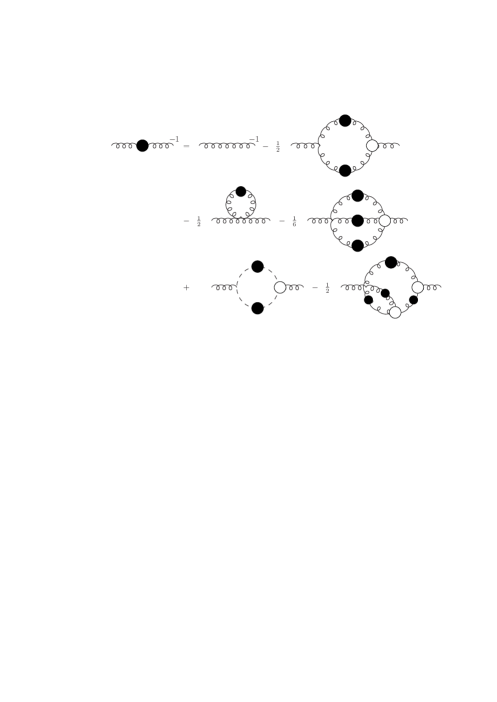
Figure 1: The complete Schwinger-Dyson equation for the gluon propagator without quarks. The spiral lines represent gluon field and the dashed lines ghosts. The black blobs are the full propagators while the white ones are the full vertices.

Actually, these unknown three and four point-functions obey their own SDE, which involve higher n-point functions which naturally must satisfy, in their turn, their own SDE. In fact, it is this entanglement of equations which makes unavoidable the use of some truncation schemes.

One famous truncation scheme is the Mandelstam’s approximation where the fermion fields are neglected, since we believe that a pure Yang-Mills theory must carry all the main features of QCD. Furthermore, based on perturbative results, the ghost fields are also neglected. The justification, for the latter approximation is that the contribution which comes from the ghost field is supposed to be small even in the non-perturbative region. Therefore, this approximation can be represented pictorially by the graphics which compound the first line of the Fig.(1) and is written as [1]

$$D^{-1\mu\nu}(k^{2})=D_{0}^{-1\mu\nu}(k^{2})$$

$$\hskip 28.45274pt+g_{0}^{2}C_{2}\frac{1}{2}\int\frac{d^{4}q}{(2\pi)^{4}}\Gamma_{0}^{\mu\rho\alpha}(k,-p,q)D_{\alpha\beta}(q^{2})D_{\rho\sigma}(p^{2})\Gamma^{\beta\sigma\nu}(-q,p,-k),$$ (1)

where $p=k+q$, $D_{0}$ and $\Gamma_{0}$ are respectively the propagator and three-gluon vertex at tree level, while $D$ and $\Gamma$ are the two and three points full Green functions. In the case of the full gluon propagator in Landau gauge, $D^{\mu\nu}$, we can write it as

$$D^{\mu\nu}(q^{2})=\left(\delta^{\mu\nu}-\frac{q^{\mu}q^{\nu}}{q^{2}}\right)\frac{{\mathcal{Z}}(q^{2})}{q^{2}},$$ (2)

where it will be useful to define the function, $D(q^{2})$, in terms of the gluon renormalization function, ${\mathcal{Z}}(q^{2})$.

$$D(q^{2})=\frac{{\mathcal{Z}}(q^{2})}{q^{2}}.$$ (3)

Neglecting all contributions coming from ghosts fields, the Slavnov-Taylor identity between the three gluon vertex and the inverse of the gluon propagator can be expressed in the following simple form

$$k_{\mu}\Gamma^{\mu\nu\rho}(k,p,q)=\frac{q^{2}}{{\mathcal{Z}}(q^{2})}\left(\delta^{\nu\rho}-\frac{q^{\nu}q^{\rho}}{q^{2}}\right)-\frac{p^{2}}{{\mathcal{Z}}(p^{2})}\left(\delta^{\nu\rho}-\frac{p^{\nu}p^{\rho}}{p^{2}}\right).$$ (4)

In order to allow that a massive gluon propagator will be also compatible with the Slavnov-Taylor identity expressed above, and supposing that the gluon renormalization function, ${\mathcal{Z}}(q^{2})$ admits an expression of the following form

$${\mathcal{Z}}(q^{2})=\frac{q^{2}}{q^{2}+m^{2}},$$ (5)

we note that it must be added new terms, that have massless poles, to the structure of the three gluon vertex, which, apart from a group theoretical factor, lead us to a first modification that we should introduce in the construction of the full vertex, which is the one prescribed by Cornwall many years ago [5]

$$\Gamma^{(m)}_{0\,\mu\nu\rho}(k,p,q)=(k-p)_{\rho}\delta_{\mu\nu}+\frac{m^{2}}{2}\frac{k_{\mu}p_{\nu}(k-p)_{\rho}}{k^{2}p^{2}}+\mbox{c.p.},$$ (6)

where $c.p.$ means cyclic permutation, and, as discussed in Ref. [5], $\Gamma^{(m)}_{0\,\mu\nu\rho}$ is the vertex for the massive theory.

As remarked by Corwnall [5], during the procedure of construction of a vertex function which automatically satisfied the Slavnov-Taylor identities, Ball and Chiu [14] have done a crucial assumption in order to get a unique form for the longitudinal vertex. They supposed that the vertex should be free of kinematic singularities, since most of these singularities violate the general analyticity requirements of the vertex. Therefore, tensorial structures which have massless poles in three gluon vertex were explicitly excluded in their construction, despite the fact that they have already mentioned in the same work, that there are certain types which might naturally occur without the breakdown of analyticity in the three gluon vertex, and one structure of this type is the one given by the second term in the right hand side of Eq.(6).

It is important to bear in mind that the mass $m$ in Eq.(6) has a momentum dependence and do not destroy the unitary behavior of the theory [5]. Moreover, as stressed before, the role of the latter term from Eq.(6), is only to allow that the gluon propagator could assume a non-zero value, i.e. $D^{-1}(q^{2}=0)\neq 0$, at the deep infrared region, without breaking the gauge invariance imposed by the Slavnov-Taylor identity. Exactly the massless poles of Eq.(6) lead to the possibility of a mass gap, contrarily to the solutions for the infrared gluon propagator behaving as $1/q^{4}$ found in Ref.[1, 15] where a different vertex choice is made.

The next step in the Mandelstam approximation is to define the final expression for the full three gluon vertex. The form of the full three gluon vertex is [3]

$$\Gamma^{\mu\nu\rho}(k,p,q)=\frac{1}{{\mathcal{Z}}(p^{2})}\Gamma^{{(m)}\,\mu\nu\rho}_{0}(k,p,q).$$ (7)

The use of the above full vertex, which is a combination of the Cornwall’s and Mandelstam’s prescriptions, simplify even more the structure of gluon SDE than the use of the bare vertex, once it implies a cancellation between the gluon renormalization function which comes from a full gluon propagator and the one that comes from the full triple vertex.

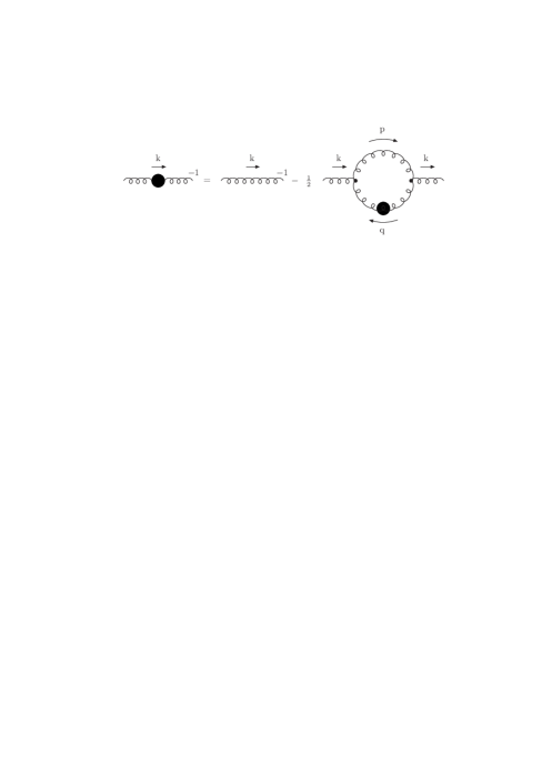
Figure 2: The gluon Schwinger-Dyson equation in the Mandelstam’s approximation.

With the above expressions for the gluon propagators and vertices and contracting this result with the projector, proposed by Brown and Pennington [3],

$${\mathcal{R}}^{\mu\nu}(k)=\delta^{\mu\nu}-4\frac{k^{\mu}k^{\nu}}{k^{2}},$$ (8)

the follow equation comes out,

$$\frac{1}{{\mathcal{Z}}(k^{2})}=1 +\frac{g_{0}^{2}}{16\pi^{2}}\int^{k^{2}}_{0}\frac{dq^{2}}{k^{2}}\left(\frac{7}{2}\frac{q^{4}}{k^{4}}-\frac{17}{2}\frac{q^{2}}{k^{2}}-\frac{9}{8}\right){\mathcal{Z}}(q^{2})$$ (9)

$$\hskip 42.67912pt+\frac{g_{0}^{2}}{16\pi^{2}}\int^{{\Lambda}^{2}}_{k^{2}}\frac{dq^{2}}{k^{2}}\,\left(\frac{7}{8}\frac{k^{4}}{q^{4}}-7\frac{k^{2}}{q^{2}}\right){\mathcal{Z}}(q^{2}),$$

where $g_{0}$ is the bare coupling, we use the color factor, $C_{2}=3$ and $\Lambda$ is an ultraviolet cutoff which was introduced in order to render the integral finite. In fact, the great advantage of the Mandelstam approximation is that all the angular integrals can be performed analytically leading us to a much simpler equation.

A remark concerning the massive term of the three gluon vertex is in order. This equation is exactly the same one obtained in Ref.[3]. Although the three gluon vertex has an extra term, no contributions come from it. Therefore, as mentioned before, its only role is to allow that the inverse gluon propagator can be different from zero at the origin consistently with the Slavnov-Taylor identity.

3 Renormalization

The procedure to perform the renormalization of SDE in the Mandelstam’s approximation consists in introducing the gluon and vertex renormalization constants, $Z_{3}$ and $Z_{g}$, respectively which will absorb ultraviolet divergences of the equation. Through these constants we can define the following renormalized quantities

$$D(q^{2},\Lambda^{2}) = Z_{3}(\mu^{2},\Lambda^{2})D_{R}(q^{2},\mu^{2})$$

$$g_{0}(\Lambda^{2}) = Z_{g}(\mu^{2},\Lambda^{2})g(\mu^{2}),$$ (10)

where $D_{R}$ and $g$ are the renormalized gluon propagator and the renormalized coupling.

Substituting into the SDE, Eq.(9), the nonrenormalized quantities, $D$ and $g_{0}$, by the renormalized ones lead us to

$$D_{R}(k^{2})=\left[k^{2}Z_{3}+Z_{3}^{2}Z_{g}^{2}\frac{g^{2}(\mu^{2})}{16\pi^{2}}{\mathcal{I}}_{D_{R}}(k^{2})\right]^{-1},$$ (11)

where ${\mathcal{I}}_{D_{R}}(k^{2})$ is given by

$${\mathcal{I}}_{D_{R}}(k^{2}) = \int^{k^{2}}_{0}dq^{2}\left(\frac{7}{2}\frac{q^{4}}{k^{4}}-\frac{17}{2}\frac{q^{2}}{k^{2}}-\frac{9}{8}\right)q^{2}D_{R}(q^{2})$$ (12)

$$\hskip 85.35826pt+\int^{{\Lambda}^{2}}_{k^{2}}dq^{2}\,\left(\frac{7}{8}\frac{k^{4}}{q^{4}}-7\frac{k^{2}}{q^{2}}\right)q^{2}D_{R}(q^{2}).$$

The vertex renormalization constant $Z_{g}$ can be eliminated from the Eq.(11), using the identity, $Z_{g}Z_{3}=1$, which is only valid in this approximation [16]. However, there still remains the gluon renormalization constant $Z_{3}$ that is a naturally divergent quantity.

Despite all efforts to obtain a totally consistent renormalization of the gluonic SDE, be it in this truncation or even beyond the Mandelstam approximation, we know that the renormalization of SDE is highly nontrivial. To illustrate this claim we notice that only in the nineties, Curtis and Pennington pointed out a truncation scheme, for QED, which is gauge independent and also respect the multiplicative renormalizability [17]. In the following we consider $Z_{3}$ as a factor which renders the divergent terms of the gluon SDE in a finite one through a subtractive renormalization.

After imposing $Z_{g}Z_{3}=1$ in Eq.(11) we are left with the following equation

$$D_{R}(k^{2})^{-1} = k^{2}\left[Z_{3}+\frac{\alpha(\mu^{2})}{4\pi}\int^{{\Lambda}^{2}}_{k^{2}}dq^{2}\,\left(-7\right)D_{R}(q^{2})\right]$$

$$+ \frac{\alpha(\mu^{2})}{4\pi}\int^{k^{2}}_{0}dq^{2}\left(\frac{7}{2}\frac{q^{4}}{k^{4}}-\frac{17}{2}\frac{q^{2}}{k^{2}}-\frac{9}{8}\right)q^{2}D_{R}(q^{2})$$

$$+ \frac{\alpha(\mu^{2})}{4\pi}\int^{{\Lambda}^{2}}_{k^{2}}dq^{2}\,\frac{7}{8}\frac{k^{4}}{q^{2}}D_{R}(q^{2})$$

where $\alpha(\mu^{2})=\frac{g^{2}(\mu^{2})}{4\pi}$. $Z_{3}$ behaves as $1$ plus an infinite piece. The factor $1$ is consistent with the perturbative behavior, and the infinite part of $Z_{3}$ must cancel the infinite part that comes out from the first integral in Eq.(3), which is the only divergent integral in the above equation.

It is important to notice that Eq.(3) is not of the same form as the one shown in Ref.[5], as well as we shall not follow the same procedure adopted up to now in the many papers to renormalize the Mandelstam equation. In the previous papers where this equation was solved it was verified that the dressing of the gluon propagator could behave as

$$Z(k^{2})=\frac{1}{A+Bk^{2}+J(k^{2})}$$ (14)

The numerical solutions were then obtained assuming $A=0$ and $B=1$, which are not independent conditions. Note that these conditions are necessary to obtain a solution compatible with the Slavnov-Taylor (ST) identities in the case of a massless gluon. As discussed in the previous section, it is possible to introduce a new piece in the gluon vertex that makes the ST identities compatible with dynamical mass generation for the gluons, alleviating any condition on $A$ and $B$.

We will face $Z_{3}$ as the term that will eliminate the infinite contribution of the following expression

$$Z_{3}-\frac{\alpha(\mu^{2})}{4\pi}\int^{\Lambda^{2}}_{k^{2}}\,dq^{2}\,7D_{R}(q^{2})\,\,\,.$$ (15)

Of course, in the above subtraction there remains a finite contribution. $D_{R}(q^{2})$ must be known to perform the above calculation, but it is going to be known only after we impose the renormalization conditions

$${\mathcal{Z}_{R}}(\mu^{2})=1,$$ (16)

or equivalently

$$D_{R}^{-1}(\mu^{2})=\mu^{2}.$$ (17)

The role of the above equation is to guarantee that exactly at the point $\mu^{2}$ we recover the bare perturbative behavior, $D_{R}(q^{2})=1/q^{2}$. For this reason it is important that the value of $\mu^{2}$ be fixed at a typical perturbative scale, i.e. it must satisfy the condition $\mu^{2}\gg\Lambda_{QCD}$.

Let us now discuss the prescription for the finite contribution to Eq.(15). The solution usually found for the Mandelstam gluon propagator is of the form $D_{1}(k^{2})\approx 1/k^{4}$. But in principle, as long as we do not impose $A=0$ and $B=1$ as discussed after Eq.(14), we cannot discard a solution behaving like $D_{2}(k^{2})\approx 1/[(k^{2}+m^{2})\ln(k^{2}+m^{2})]$, which is a massive solution similar to the one found by Cornwall in Ref.[5].

If $D_{R}(q^{2})$ behaves as $D_{1}(q^{2})$ it is natural to have a finite contribution like $\kappa_{1}/k^{2}$ in the integration of Eq.(15). The same is true for high values of $k^{2}$ if $D_{R}(q^{2})$ behaves as $D_{2}(q^{2})$, since the integral that appears in Eq.(15) will generate terms like $\ln\ln\Lambda^{2}$, $\ln\ln k^{2}$ and again a term proportional to $m^{2}/k^{2}$. It is also not likely that the integral in Eq.(15) will give finite contributions like $\delta_{n}/(k^{2})^{n}$ with $n\geq 2$, because this behavior is not consistent with any expected form of $D_{R}(q^{2})$. As $\kappa_{1}$ and $m^{2}$ have exactly the same dimension, the simplest form of Eq.(15)which is compatible with both behaviors is

$$Z_{3}-\frac{\alpha(\mu^{2})}{4\pi}\int^{\Lambda^{2}}_{k^{2}}\,dq^{2}\,7D_{R}(q^{2})=1+\frac{\kappa}{k^{2}}\,\,,$$ (18)

where $\kappa$ has squared mass dimension and is going to be fixed by the renormalization procedure ($D_{R}^{-1}(\mu^{2})=\mu^{2}$).

A more complex expression on the right-hand side would introduce new constants besides $\kappa$, which could be fixed only in an ad hoc fashion. The $1$ in the right-hand side of the above expression corresponds to the first $Z_{3}$ term. The choice we made in Eq.(18) does not obey the conditions $A=0$ and $B=1$ that we discussed before, and, in principle, it allows even for a massive gluon solution. This possibility is an actual one as long as we obtain a stable solution for the final equation.

In all the procedures used up to now to solve the Mandelstam equation, it has been assumed a cancellation of certain terms, and there is not any discussion about the finite terms that survive renormalization. It is known that in perturbative calculations such finite terms are nothing else than small quantum corrections which modifies the tree level value of the renormalized quantity. On the other hand the physical quantities which are related to the non-perturbative dynamical mass generation will be exclusively generated by the quantum corrections. This means that such finite terms surviving renormalization are fundamental to the final result.

With the definition described by the Eq.(18) and imposing the renormalization condition (17) into Eq.(3) we can obtain the following expression for the parameter $\kappa$,

$$\kappa=- \frac{\alpha(\mu^{2})}{4\pi}\int^{\mu^{2}}_{0}dq^{2}\left(\frac{7q^{4}}{2\mu^{4}}-\frac{17q^{2}}{2\mu^{2}}-\frac{9}{8}\right)q^{2}D_{R}(q^{2})$$ (19)

$$\hskip 85.35826pt-\frac{\alpha(\mu^{2})}{4\pi}\int^{\Lambda^{2}}_{\mu^{2}}dq^{2}\frac{(7\mu^{4})}{8q^{4}}q^{2}D_{R}(q^{2})$$

and, consequently, the final expression for the inverse of the gluon propagator can be written as

$$D_{R}^{-1}(k^{2})=\kappa+k^{2}+ \frac{\alpha(\mu^{2})}{4\pi}\int^{k^{2}}_{0}dq^{2}\left(\frac{7q^{4}}{2k^{4}}-\frac{17q^{2}}{2k^{2}}-\frac{9}{8}\right)q^{2}D_{R}(q^{2})$$

$$+ \frac{\alpha(\mu^{2})}{4\pi}\int^{\Lambda^{2}}_{k^{2}}dq^{2}\frac{7k^{4}}{8q^{4}}q^{2}D_{R}(q^{2}).$$ (20)

Since we are now dealing only with renormalized quantities, in the sequence we will dismiss the subscript $R$ in the Green functions in order to get a more compact notation. It is interesting to note that the renormalization constant $Z_{3}$ as it is established by Eq.(18) is proportional to $1$ plus a function of $\mu^{2}$ and $\Lambda^{2}$. Such behavior is compatible with the expected weak coupling expansion for this constant.

As already stated, the renormalization procedure in Schwinger-Dyson equations has an intricate structure and other choices have already been applied in these equations, such as the “plus prescription” [18] where the contributions which violate the massless Slavnov-Taylor identity would be subtracted out of the right hand side of Eq.(9) or even in more elaborated cases, as the gluon-ghost coupled system, where we have to deal with a bigger number of renormalization constants, different approaches can be considered [6, 19]. As long as we do not have an exact procedure for the renormalization problem in non-Abelian SDE, we have to face this prescription as one more try, that certainly can be improved, where the quantitative perturbative behavior of the renormalization constant $Z_{3}$ is reproduced.

Our prescription in Eq.(18) acts as a seed for the dynamical gluon mass generation, since $\kappa$ defined by Eq.(19) is precisely a constant, like the $A$ term in Eq.(14). Of course, this is not the most general prescription, and it does not reproduce the exact perturbative ultraviolet behavior of the gluon propagator. This behavior can be obtained if we use the following prescription

$$Z_{3}-\frac{\alpha(\mu^{2})}{4\pi}\int^{\Lambda^{2}}_{k^{2}}\,dq^{2}\,7D_{R}(q^{2})=1+\frac{\kappa_{1}}{k^{2}}+\frac{4\pi}{\beta_{0}}\ln{\frac{k^{2}}{\kappa_{2}}}\,\,.$$ (21)

It is clear that the last term of Eq.(21) arises naturally from the integration of the perturbative propagator ($D(q^{2})=1/q^{2}$) in Eq.(15). However, the new constant ($\kappa_{2}$) cannot be fixed, since we have only one renormalization condition. In the next section we shall discuss the effect of a term like this one.

Before starting the numerical calculation of the gluon propagator, it is useful to remind the definition of the running coupling that will be valid from the non-perturbative to the perturbative region. Remembering that, in the Mandelstam approximation, $Z_{3}Z_{g}=1$, it follows from Eq.(10) that

$$\alpha(q^{2})=\alpha(\mu^{2})\left[\frac{{\mathcal{Z}}(q^{2})}{{\mathcal{Z}}(\mu^{2})}\right]^{2},$$ (22)

where we assume that ${\mathcal{Z}}(\mu^{2})=1$.

It is important to keep in mind that, in QCD, we have the possibility to define the running coupling constant using the different vertices of the theory, such as, the three gluon, four gluon, ghost-gluon or even the fermion-gluon vertices. Despite the fact that in the perturbative QCD all these constructions, based on different vertices, converge to the same behavior for the running coupling, since the Slavnov-Taylor identities are preserved, the same does not happen in the low energy scale, due to the complex renormalization procedure in the infrared region of QCD, which cause the loss of the multiplicative renormalizability. As a consequence we may not have a unique definition for the running coupling in the infrared region. For this reason it is important to stress that, in this approximation, our QCD running coupling is constructed on the basis of three-gluon vertex, since all the others vertices do not appear in this approximation.

In the sequence we shall need the perturbative expression for the running coupling, which is given by

$$\alpha(q^{2})=\frac{4\pi}{\beta_{0}\ln\left(\frac{q^{2}}{\Lambda_{QCD}^{2}}\right)},$$ (23)

where $\Lambda_{QCD}$ is the usual scale for QCD and $\beta_{0}$ is the first coefficient of the the Callan-Symanzik $\beta$ function, $\beta(g)=\mu(dg/d\mu)$, which is written as

$$\beta(g)=-\beta_{0}\frac{g^{3}}{16\pi^{2}}-\beta_{1}\frac{g^{5}}{(16\pi^{2})^{2}}+\ldots,$$ (24)

where the $\beta_{0}$ and $\beta_{1}$ coefficients are given by

$$\beta_{0} = 11-\frac{2}{3}n_{f}$$

$$\beta_{1} = 102-\frac{38}{3}n_{f}.$$ (25)

Since we neglected the fermions fields, we have that $n_{f}=0$ which lead us to $\beta_{0}=11$ at one loop.

4 The massive solution

It has been shown in several works that it is not an easy task to obtain an analytical solution for the Eq.(20) [1, 3, 6] and therefore the only possibility to face this problem is through a numerical approach.

Our aim here is to find consistent solutions over the whole momentum range without impose, neither in the infrared region nor in the ultraviolet, any previous asymptotic behavior obtained from an expansion of the gluon renormalization function, ${\mathcal{Z}}(q^{2})$, at small $q^{2}$ or obtained from the known perturbative behavior.

For this reason, we apply for the integral equation, given by Eq.(20), an iterative numerical method, starting with a trial function which can be too remote from the exact solution.

To implement so, it is convenient to introduce the following variables $x=k^{2}$ and $y=q^{2}$ in the Eq.(20), and we also recall that since the beginning of this article all variables are in the Euclidean space, with these changes we can write Eq.(20) as

$$D^{-1}(x)=\kappa+x+\lambda\int^{x}_{0}dy\left(\frac{7y^{2}}{2x^{2}}-\frac{17y}{2x}-\frac{9}{8}\right)yD(y)+\lambda\int^{\Lambda^{2}}_{x}dy\left(\frac{7x^{2}}{8y^{2}}\right)yD(y)$$ (26)

where

$$\kappa=-\lambda\int^{\mu^{2}}_{0}dy\left(\frac{7y^{2}}{2\mu^{4}}-\frac{17y}{2\mu^{2}}-\frac{9}{8}\right)yD(y)-\lambda\int_{\mu^{2}}^{\Lambda^{2}}dy\left(\frac{7\mu^{4}}{8y^{2}}\right)yD(y),$$ (27)

with $\lambda=\alpha(\mu^{2})/{4\pi}$.

In order to study, in more details, the small $x$ region, we use a logarithmic grid for the variables $x$ and $y$, which allow us to vary the momentum from the deep infrared to the ultraviolet region. Such logarithmic grid split the whole momenta range in two regions: the infrared region - defined by the range $[0,\mu^{2}]$ and the ultraviolet that comprehends the range $[\mu^{2},\Lambda^{2}]$. The aim of this separation is to allow us to set ${\mathcal{Z}}(\mu^{2})=1$ or equivalently, $D^{-1}(\mu^{2})=\mu^{2}$ [21].

We start with a trial function $D(x)$ and use a cubic spline interpolation for generating the values of $D(y)$ which will be utilized in the right hand side of the Eq.(27) and in the sequence we compute this integral through the Adaptive Richardson-Romberg extrapolation.

The initial trial function is compared with the result which was obtained after the integration and the convergence criteria to stop the numerical code is to impose that the difference between input and output functions must be smaller than $10^{-4}$.

It is important to stress that we have tested variations of initial guesses and verified that our results are completely independent of the trial function imposed for $D(x)$.

We also analyzed the solution proposed in Ref.[3] and we noticed that it can only be reproduced if we consider exactly the same momentum range showed in their Fig.3 (as is already stressed in Ref.[16]) and use a trial function which is very close to the result found in [3]. Such exigency reflects the instability of this solution, because if we extend the numerical range or even start from a different guess we do not recover the divergent $1/k^{4}$ behavior.

Our input data are the renormalization point, $\mu^{2}$, and the coupling constant defined at this point, $\alpha(\mu^{2})$, which has the effect of fixing the value of the QCD scale, $\Lambda_{QCD}$, through the Eq.(23).

As stressed in the Sec.(3), the value of $\mu^{2}$ must be fixed at a typical perturbative scale in order to recover the high energy behavior of the gluon propagator. With the aim of analyze the dependency of our solution on the renormalization point, we vary the values of $\mu^{2}$ and $\alpha(\mu^{2})$ within the range $[10\,\mbox{GeV}^{2},30\,\mbox{GeV}^{2}]$ and $[0.20,0.25]$ respectively. Such variation correspond to run the $\Lambda_{QCD}$ parameter from $182\,\mbox{MeV}$ to $557\,\mbox{MeV}$ as we show in the Table(1).

The curves produced by these different scales are plotted in the Fig.(3) where it is shown the gluon propagator, $D(q^{2})$, as a function of the momentum $q^{2}$. The external curves delimit the lower and the higher values of the $\Lambda_{QCD}$ in the range mentioned above. The other set of input, shown in the Table(1), reproduce the same qualitative behavior and they are restricted to the shadow band.

We have also computed the case where $\alpha(\mu^{2})$ is fixed at the bottom quark mass, $m_{b}^{2}=(4.5)^{2}\,\mbox{GeV}^{2}$, and its central value is $\alpha(m_{b}^{2})=0.22$ [22], such solution is represented by the curve “line + circle” displayed on the Fig.(3).

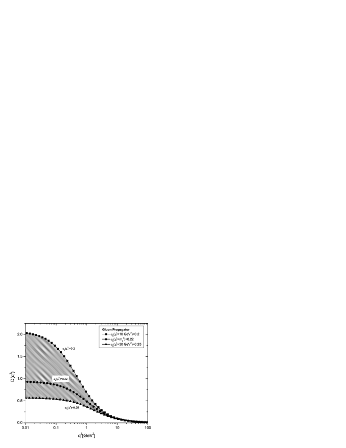
Figure 3: Gluon propagator, $D(q^{2})$, as function of momentum $q^{2}$ for different scales. The line + square curve was obtained when $\alpha(10\,\mbox{GeV}^{2})=0.2$ which corresponds $\Lambda_{QCD}=182\,\mbox{MeV}$, while in the line + triangle curve, $\alpha(30\,\mbox{GeV}^{2})=0.25$, which leads to $\Lambda_{QCD}=557\,\mbox{MeV}$. The shadowed area delimits the curves with $\Lambda_{QCD}$ varying within the range $[182\,\mbox{MeV},557\,\mbox{MeV}]$. The central curve (line + circle) was obtained when we fix the renormalization point, $\mu^{2}$, at bottom quark mass, $m_{b}^{2}=(4.5)^{2}\,\mbox{GeV}^{2}$ with the central value of $\alpha(m_{b}^{2})=0.22$.

We have run our numerical code efficiently within a momenta range of twelve orders of magnitude where the typical momenta values which were utilized vary from $10^{-6}$ to $10^{6}\,\mbox{GeV}^{2}$. We set the renormalization point at $m_{b}^{2}$, which is located approximately in the middle of our typical momenta range, and where the physical quantities can be certainly described by the perturbative theory.

It is interesting to provide an analytic expression for the gluon propagator, in order to analyze the gluon mass values obtained in infrared region, when we set the renormalization point, $\mu^{2}$, at different values. With this aim we fit our numerical data by an Euclidean massive propagator expressed by [5]

$$D(q^{2})=\frac{4\pi}{\beta_{0}\left(q^{2}+m^{2}(q^{2})\right)\ln\left(\frac{q^{2}+4m^{2}(q^{2})}{\Lambda_{QCD}}\right)},$$ (28)

where

$$m^{2}(q^{2})=m^{2}_{0}\left[\frac{\ln\left(\frac{q^{2}+4m_{0}^{2}}{\Lambda_{QCD}^{2}}\right)}{\ln\left(\frac{4m_{0}^{2}}{\Lambda_{QCD}^{2}}\right)}\right]^{-12/11}.$$ (29)

We have also considered the simpler expression

$$D(q^{2})=\frac{1}{q^{2}+{\mathcal{M}}^{2}(q^{2})},$$ (30)

where the dynamical mass ${\mathcal{M}}^{2}(q^{2})$ is described by

$${\mathcal{M}}^{2}(q^{2})=\frac{{m^{\prime}}^{4}}{q^{2}+{m^{\prime}}^{2}}.$$ (31)

The last fit can be motivated by the gluon polarization tensor behavior at high energies, which can be predicted by OPE as [23]

$$\Pi_{OPE}(P^{2})\sim-\frac{34N\pi^{2}}{9(N^{2}-1)}\frac{\left\langle{\frac{\alpha_{s}}{\pi}}G^{\mu\nu}G_{\mu\nu}\right\rangle}{P^{2}}.$$ (32)

On the other hand recently there has been a lot of discussion about a possible bilinear condensate of the gluon field [24]. Such condensate, $\left\langle A^{\mu}A_{\mu}\right\rangle$, would be responsible for a mass term appearing in the infrared gluon polarization tensor [24]. Therefore the fit provided by Eq.(31) is just the simplest way to account for the different condensate contributions to the polarization tensor, from where we could expect approximate relations of the form ${m^{\prime}}^{2}\propto\left\langle A^{\mu}A_{\mu}\right\rangle$ or ${m^{\prime}}^{4}\propto\left\langle{\frac{\alpha_{s}}{\pi}}G^{\mu\nu}G_{\mu\nu}\right\rangle$. We will discuss such type of relation in the next section.

We can apply these simple fits for all curves shown in the Fig.(3) and in all cases it is remarkable the agreement found from the deep infrared region up to the ultraviolet regime, using a fit which has a unique parameter, $m_{0}$ or $m^{\prime}$.

In particular, we plot in the Fig.(4) the numerical solution for the gluon propagator, $D(q^{2})$, when $\mu^{2}=m_{b}^{2}$ together with the curve obtained through our fit given by Eqs.(30) and (31) when ${m^{\prime}}^{2}=1.11\,\mbox{GeV}^{2}$ as well as the fit provided by the Eqs.(28) and (29) when ${m_{0}}^{2}=0.82\,\mbox{GeV}^{2}$.

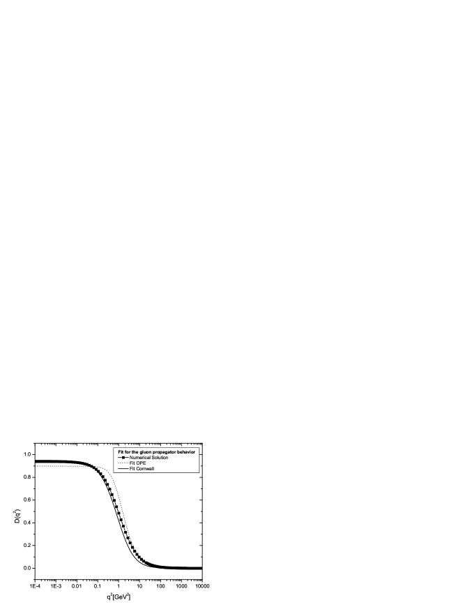
Figure 4: Numerical solution for the gluon propagator, $D(q^{2})$, versus momentum $q^{2}$ for $\alpha(m^{2}_{b})=0.22$. We compare this numerical solution with the fit given by Eq.(30), where ${m^{\prime}}^{2}=1.11\,\mbox{GeV}^{2}$, as well as the one given by the Eqs.(28) and (29) when ${m_{0}}^{2}=0.82\,\mbox{GeV}^{2}$.

In particular we can easily extract the value of ${m^{\prime}}$ for the others curves displayed in the Fig.(3), to do so we basically have just to note that in the limit of $q^{2}\rightarrow 0$, Eqs.(30) and (31) of our gluon propagator reduces to $D(q^{2}\rightarrow 0)=1/{m^{\prime}}^{2}$, and therefore the inverse of ${m^{\prime}}^{2}$ is given by the value of the point in what the gluon propagator curves cross the y axis in Fig.(3).

We verified that the value of $m_{0}$ and ${m^{\prime}}$ depend on the choice of the renormalization point, $\mu^{2}$, however we must remember that when we change its value, actually what we are really changing is the scale of the theory, once that $\mu^{2}$ and $\Lambda_{QCD}$ are linked by Eq.(23). For this reason what matters is the analysis of the ratio $m_{0}/\Lambda_{QCD}$ or ${m^{\prime}}/\Lambda_{QCD}$ which, in principle, give to us a better idea about the true dependency on the renormalization point of our solution.

Fixing the coupling constant and running the renormalization point we can see from the Table(1) that the aforementioned ratios practically do not vary for the set of coupling constants shown in the table. This means that the ratios $m_{0}/\Lambda_{QCD}$ ${m^{\prime}}/\Lambda_{QCD}$ are quite stable in our procedure.

Table 1: Values of the renormalization point, $\mu^{2}$, and coupling constant, $\alpha(\mu^{2})$, used as input data in the Eq.(27). In the third column, we have the values of $\Lambda_{QCD}$ computed with the usual perturbative value of $\beta_{0}=11$. The values of the ratios $m_{0}/\Lambda_{QCD}$ and $m^{\prime}/\Lambda_{QCD}$ are also shown in the last two columns.

$\alpha(\mu^{2})$	$\mu^{2}$	$\Lambda_{QCD}$	${m_{0}}/{\Lambda_{QCD}}$	${m^{\prime}}/{\Lambda_{QCD}}$
		$(\beta=11)$	Cornwall	OPE
$0.20\qquad$	$10\,\mbox{GeV}^{2}$	$182\,\mbox{MeV}\qquad$	$3.18$	$3.90$
$0.20\qquad$	$20\,\mbox{GeV}^{2}$	$257\,\mbox{MeV}\qquad$	$3.18$	$3.90$
$0.20\qquad$	$30\,\mbox{GeV}^{2}$	$315\,\mbox{MeV}\qquad$	$3.18$	$3.90$
$0.22\qquad$	$m_{b}^{2}=20.25\,\mbox{GeV}^{2}$	$335\,\mbox{MeV}\qquad$	$2.70$	$3.15$
$0.25\qquad$	$10\,\mbox{GeV}^{2}$	$321\,\mbox{MeV}\qquad$	$2.23$	$2.45$
$0.25\qquad$	$20\,\mbox{GeV}^{2}$	$455\,\mbox{MeV}\qquad$	$2.28$	$2.44$
$0.25\qquad$	$30\,\mbox{GeV}^{2}$	$557\,\mbox{MeV}\qquad$	$2.23$	$2.43$

We have also checked the effect of the prescription shown in Eq.(21) attributing random values to $\kappa_{2}$. We also obtained massive solutions with a better ultraviolet behavior. The numerical curves are totally identical to the ones in Fig.(3) but they scale up or down by a constant factor as we change the value of $\kappa 2$. The only way to eliminate such constant is forcing point by point of the numerical solution in the large momentum region to match with the curve given by the known asymptotic perturbative solution.

We now turn to the infrared behavior of the coupling constant which was built based on the triple gluon vertex as outlined above. By imposing the limit $q^{2}\rightarrow 0$ in the Eq.(22) where the renormalization function, ${\mathcal{Z}}(q^{2})$, can be extracted from the fit which is expressed by Eq.(30) and (31) we clearly obtain a vanishing coupling in the deep infrared region within the Mandelstam approximation. Although it may look surprising to find that in a confining theory the IR coupling constant goes to zero, it is important to stress again that, for QCD, we have distinct definitions for $\alpha(q^{2})$ which are based on different vertices of the theory, moreover it is interesting to say that using the same vertex, a lattice QCD simulation found the same vanishing behavior for the coupling [25]. Of course, the introduction of ghosts can modify this result, and it seems unlikely then that this limit does reflect the true behavior of the coupling constant since we know that it must develop a non-trivial fixed point in QCD infrared region [12].

Following the same procedure that are perfomed here, the qualitative behavior of the gluon propagator does not change when the ghosts fields are included when we study the coupled SDE for the gluon and ghost [26]. We believe that the main role of the ghost fields in covariant gauges is to guarantee that the coupling constant will be finite and different from zero in the infrared regime, although it is quite hard to obtain numerically this freezing of the coupling without imposing any previous asymptotic form for the gluon and ghost propagators .

5 Vacuum energy and stability of the solution

In this section we would like to discuss some points about the stability of the massive solution in this approximation. We call attention to the fact that our solution is obtained numerically in the full range of momenta. Other solutions for this kind of equations in general assume one particular form of the solution in the far infrared region and adjust free parameters in a “in” and “out” procedure. We notice that our numerical code finds stability for the $1/q^{4}$ solution found in Ref.[3] only when we enter in the code a seed basically given by the final result of Ref.[3], otherwise there is no convergence up to a large computing time. We credit this behavior to the fact the $1/q^{4}$ must be an unstable solution of the SDE in this approximation, because any seed that is slightly away from the result of Ref.[3] does not lead to a convergent calculation. Unfortunately we cannot say more than that about the stability of the $1/q^{4}$ solution.

It is possible to use some methods of integral equations to study the existence and stability of the solutions as in Ref.[27], but these methods may depend on the many approximations that are necessary to make in order to obtain a tractable equation before they can be applied. We believe that the best to be done is to compute the vacuum energy for composite operators [28]. This vacuum energy is a function of the full propagator and vertices of the theory [28, 29]. The idea is simply to recall that the vacuum energy will select the solution that leads to the deepest minimum of energy as discussed in Ref.[30] in the case of pure gauge QCD. If we follow the results of Ref.[30] we can foresee that the massive solution is the one selected by the vacuum. However we can do more than that and we will show that the computation of the vacuum energy obtained in the previous section also leads to a consistent value for the gluon condensate.

We will briefly outline the calculation of the vacuum energy with the formalism of the effective potential for composite operators [28]. It will also be computed according to the Mandelstam’s approximation, what is equivalent to neglect diagrams with fermions, ghosts and the quadrilinear gauge coupling. The details can be obtained in Ref.[31]. The effective potential with the approximations already discussed has the form [28]

$$V(D)=\frac{\imath}{2}\int\frac{d^{4}p}{(2\pi)^{4}}Tr(\ln D_{0}^{-1}D-D_{0}^{-1}D+1)+V_{2}(D),$$ (33)

where $D(D_{0})$ is the complete(bare) gluon propagator, $V_{2}(D)$ is a two-particle irreducible vacuum diagram and the equation

$$\frac{\delta V}{\delta D}=0,$$ (34)

gives the SDE for gauge bosons in the Mandelstam’s approximation.

The two-loop contribution to $V_{2}(D)$ is given by

$$V_{2}(D)=\frac{-\imath}{6}Tr(\Gamma^{(3)}D\Gamma^{(3)}DD),$$ (35)

where $\Gamma^{(3)}$ is the trilinear gauge boson coupling [30], and in Eq.(35) we have not written the gauge and Lorentz indices, as well as the momentum integrals.

The vacuum energy density is given by the effective potential calculated at minimum subtracted by its perturbative part, which does not contribute to dynamical mass generation  [28, 29]

$$\left\langle\Omega\right\rangle=V_{min}(D)-V_{min}(D_{p}),$$ (36)

where $D_{p}$ is the perturbative counterpart of $D$. It is easy to see that [31]

$$\left\langle\Omega\right\rangle=-\frac{3(N^{2}-1)}{2}\int\frac{d^{4}P}{(2\pi)^{4}}\,\left[\frac{\Pi}{P^{2}+\Pi}-\ln\left(1+\frac{\Pi}{P^{2}}\right)+\frac{2}{3}\frac{\Pi^{2}}{P^{2}(P^{2}+\Pi)}\right],$$ (37)

where all the quantities are in Euclidean space, $N=3$ for QCD and $\Pi$ is the gluon polarization tensor. We will compute Eq.(37) with $\Pi={\mathcal{M}}^{2}(P^{2})$, where ${\mathcal{M}}^{2}(P^{2})$ is given by Eq.(31) with $m^{\prime 2}=0.50\,\mbox{GeV}^{2}$, with the coupling constant, $\alpha(\mu^{2}=10\,\mbox{GeV}^{2})=0.20$. We obtain

$$\frac{\left\langle\Omega\right\rangle}{\Lambda^{4}_{QCD}}=3.60\,.$$ (38)

with $m^{\prime}/\Lambda_{QCD}=3.90$.

Let us recall that the vacuum expectation value of the trace of the energy momentum tensor of QCD is [32]

$$\left\langle\Theta_{\mu\mu}\right\rangle=\frac{\beta(g)}{2g}\left\langle G_{\mu\nu}G^{\mu\nu}\right\rangle,$$ (39)

where the perturbative $\beta(g)$ function up to two loops is given by Eq.(24), where the coefficients $\beta_{0}$ and $\beta_{1}$ are expressed in Eq.(25), and with $\alpha(\mu^{2})=g^{2}(\mu^{2})/4\pi$.

We can relate the Eq.(39) to the vacuum energy through

$$\left\langle\Omega\right\rangle=\frac{1}{4}\left\langle\Theta_{\mu\mu}\right\rangle.$$ (40)

This last expression for $\left\langle\Omega\right\rangle$ can be compared with the value of Eq.(38) and in this way we obtain one estimative of the gluon condensate.

Using Eq.(24) and Eq.(25) with $n_{f}=5$ (assuming that the inclusion of fermions does not change drastically our results) and using $\alpha(\mu^{2}=10\,\mbox{GeV}^{2})=0.20$ (equivalent to $m^{\prime}/\Lambda_{QCD}=3.90$) we have found the following value

$$\left\langle{\frac{\alpha_{s}}{\pi}}G^{\mu\nu}G_{\mu\nu}\right\rangle=0.015\,\,\,\mbox{GeV}^{4}.$$ (41)

We obtained this last value with $\Lambda_{QCD}=182\,\,\mbox{MeV}$ in the left hand side of Eq.(38) consistent with the perturbative value shown in the third column of Table I. The outcome of this procedure is quite close to the value commonly used in QCD sum rules [33]:

$$\left\langle{\frac{\alpha_{s}}{\pi}}G^{\mu\nu}G_{\mu\nu}\right\rangle=0.012\,\,\,\mbox{GeV}^{4}.$$ (42)

The above result indicates that our approximation gives a reliable estimative of the vacuum energy and that the inclusion of ghosts possibly do not modify the value of the vacuum energy [26].

6 Conclusion

We computed the SDE for the gluon propagator in the Landau gauge within the Mandelstam approximation where the fermions and ghost fields are neglected, and where the full gluon vertex is inversely proportional to the gluon renormalization function.

The full triple gluon vertex is also extended to include the possibility of dynamical mass generation, according to a prescription formulated by Cornwall many years ago. This prescription does not modify the SDE but is responsible for the compatibility of a massive gluon propagator with the Slavnov-Taylor identity.

The renormalization of the SDE follows a procedure similar to the one proposed by Cornwall in the renormalization of the SDE in the light cone gauge. It is particularly suited for a massive case and leads to a renormalization constant of the form $Z_{3}=1+f(\mu^{2},\Lambda^{2})$.

We were able to obtain a numerical solution in the full range of momenta that we have considered without the need of introducing any asymptotic expression for the solution. The propagator is renormalized using the central value of the coupling constant at the b quark mass. The solution has been checked to be stable within a momentum range of twelve orders of magnitude.

We verified that the ratio between the dynamical gluon mass and the QCD scale ($m/\Lambda_{QCD}$) up to a large extent is independent on the choice of the renormalization point, and its value ($m/\Lambda_{QCD}\sim 2-3$) is consistent with previous estimates for this mass [5].

Using a fit to the numerical solution we computed the vacuum energy and associated it with the gluon condensate. The value that we obtain is consistent with the one usually assumed in QCD sum rules.

Our calculation is far from being complete and the most obvious extension is the introduction of ghosts. An analysis of this case shows that the behavior of the gluon propagator is not modified by the inclusion of the ghosts fields. However the behavior of the running coupling constant as $q^{2}\rightarrow 0$ may be different from zero as happens in the present case [26].

7 Acknowledgments

We benefited from discussions with A. Cucchieri and G. Krein and we would also like to thank A. Colato for his numerical hints. This research was supported by the Conselho Nacional de Desenvolvimento Científico e Tecnológico (CNPq) (AAN) and by Fundação de Amparo à Pesquisa do Estado de São Paulo (FAPESP) (ACA).

References

- [1] S. Mandelstam, Phys. Rev. D20 (1979) 3223.
- [2] G. B. West, Phys. Lett. B115 (1982) 468.
- [3] N. Brown and M. R. Pennington, Phys. Rev. D38 (1988) 2266 ; D39 (1989) 2723 .
- [4] P. Marenzoni, G. Martinelli, N. Stella, e M. Testa, Phys. Lett. B318 (1993) 511; C. Alexandrou, Ph. de Forcrand and E. Follana, Phys. Rev. D65 (2002) 114508; D65 (2002) 117502; F. D. R. Bonnet et al., Phys. Rev. D64 (2001) 034501; D62 (2000) 051501; D. B. Leinweber et al. (UKQCD Collaboration), Phys. Rev. D58 (1998) 031501; C. Bernard, C. Parrinello, and A. Soni, Phys. Rev. D49 (1994) 1585; see also the most recent simulation of P. O. Bowman et al., hep-lat/0402032 and the references therein.
- [5] J. M. Cornwall, Phys. Rev. D26 (1982) 1453; J. M. Cornwall and J. Papavassiliou, Phys. Rev. D40 (1989) 3474; D44 (1991) 1285.
- [6] R. Alkofer and L. von Smekal, Phys. Rept. 353 (2001) 281; L. von Smekal, A. Hauck and R. Alkofer, Ann. Phys. 267 (1998) 1; L. vonSmekal, A. Hauck and R. Alkofer, Phys. Rev. Lett. 79 (1997) 3591.
- [7] T. Kugo and I. Ojima, Prog. Theor. Phys. Suppl. 66 (1979) 1.
- [8] P. Watson and R. Alkofer, Phys. Rev. Lett. 86 (2001) 5239.
- [9] K.-I. Kondo, hep-th/0303251.
- [10] J. C. R. Bloch, Few Body Syst. 33 (2003) 111.
- [11] J. Gattnar, K. Langfeld and H. Reinhardt, hep-lat/0403011.
- [12] A. C. Aguilar, A. A. Natale and P. S. Rodrigues da Silva, Phys. Rev. Lett. 90 (2003) 152001.
- [13] S. J. Brodsky, hep-ph/0310289.
- [14] J. S. Ball and Ting-Wai Chiu, Phys. Rev. D22 (1980) 2542.
- [15] R. Anishetty, M. Baker, S. K. Kim, J. S. Ball and F. Zachariasen, Phys. Lett. B86 (1979) 52; J. S. Ball and F. Zachariasen, Phys. Lett. B95 (1980) 273.
- [16] A. Hauck, L. von Smekal and R. Alkofer, Comput. Phys. Commun. 112 (1998) 149.
- [17] D. C. Curtis and M. R. Pennington, Phys. Rev. D42 (1990) 4165.
- [18] N. Brown and M. R. Pennington, Phys. Lett. B202 (1988) 257.
- [19] J. C. R. Bloch, Phys. Rev. D64 (2001) 116011; D. Atkinson, J.C.R. Bloch, Phys. Rev. D58 (1998) 094036.
- [20] M. R. Pennington, Rept. Prog. Phys. 46 (1983) 393.
- [21] A. G. Williams, G. Krein and C. D. Roberts, Annals Phys. 210 (1991) 464.
- [22] K. Hagiwara et al., Phys. Rev. D66 (2002) 010001; M. Jamin and A. Pich, Nucl. Phys, B507 (1997) 334.
- [23] M. Lavelle, Phys. Rev. D44 (1991) R26.
- [24] D. Dudal et al., JHEP 0401 (2004) 044; M. Esole and F. Freire, Phys. Rev. D69 (2004) 041701; hep-th/0401055
- [25] Ph. Boucaud et al., Nucl. Phys. Proc. Suppl. 106 (2002) 266; D.V. Shirkov, Theor. Math. Phys. 132 (2002) 1309.
- [26] A. C. Aguilar and A. Natale, JHEP 0408 (2004) 057.
- [27] D. Atkinson, J. K. Drohm, P. W. Johnson and K. Stam, J. Math. Phys. 22 (1981) 2704; D. Atkinson, P. W. Johnson and K. Stam, J. Math. Phys. 23 (1982) 1917.
- [28] J. M. Cornwall, R. Jackiw and E. Tomboulis, Phys. Rev. D10 (1974) 2428.
- [29] J. M. Cornwall and R. E. Norton, Phys. Rev. D8 (1973) 3338.
- [30] J. C. Montero, A. A. Natale and P. S. Rodrigues da Silva, Phys. Lett. B406 (1997) 130.
- [31] E. V. Gorbar and A. A. Natale, Phys. Rev. D61 (2000) 054012.
- [32] R. Crewther, Phys. Rev. Lett. 28 (1972) 1421; M. Chanowitz and J. Ellis, Phys. Lett. B40 (1972) 397; J. C. Collins, A. Duncan and S. D. Joglekar, Phys. Rev. D16 (1977) 438.
- [33] M. A. Shifman, A. I. Vainshtein and V. I. Zakharov, Nucl. Phys. B147 (1979) 385, 448.