LU TP 04-20

hep-ph/0405025

May 2004

Isospin Breaking in $K\to 3\pi$ Decays I:
Strong Isospin Breaking

Johan Bijnens and Fredrik Borg
Department of Theoretical Physics, Lund University

Sölvegatan 14A, S 22362 Lund, Sweden

The CP conserving amplitudes for the decays $K\to 3\pi$ are calculated in Chiral Perturbation Theory. The calculation is made at the next-to-leading order including strong and local electromagnetic isospin breaking. A comparison is made between the squared amplitudes with and without isospin violation to estimate the size of the effect. We find corrections of order five percent in the amplitudes.

PACS numbers: 13.20.Eb; 12.39.Fe; 14.40.Aq; 11.30.Rd

1 Introduction

Chiral Perturbation Theory (ChPT) is the effective field theory of the low-energy strong interactions. It was introduced in its present form by Weinberg, Gasser and Leutwyler [1, 2, 3] and it has had many successes and applications. A pedagogical introduction can be found in [4]. The theory has been applied as well for nonleptonic weak decays. The main work of extending ChPT to the nonleptonic weak interaction was done by Kambor, Missimer and Wyler who worked out the general formalism [5] and applied it to $K\to 2\pi,3\pi$ decays [6]. These results were then used to obtain directly relations between physical observables in [7]. Reviews of applications of ChPT to nonleptonic weak interactions are [8]. The expressions of Ref. [6] were never published and have been lost.

The next-to-leading order $K\to 2\pi$ amplitudes in the isospin limit were recalculated in [9, 10] and the $K\to 3\pi$ amplitudes in [10]. The latter have been confirmed in [11]. In [10] a full fit to all available $K\to 2\pi$ and $K\to 3\pi$ experimental results was performed and it was found that one could fit the decay rates and the slopes in the Dalitz plot. There was a discrepancy with the observed quadratic slopes or curvatures in the Dalitz plot and this can have several different origins. It could be an experimental problem (especially given the discrepancies between several experiments) or it could have a theoretical origin. In the latter the amplitudes calculated so far have three different types of corrections, isospin breaking, electromagnetic corrections or higher order ChPT corrections. In this paper we investigate the first class. Work is in progress to evaluate the electromagnetic corrections as well. More precisely, in this paper we investigate effects of the quark mass difference $m_{u}-m_{d}$ as well as the local electromagnetic effects. We have worked out all orders in $m_{u}-m_{d}$ to order four in the chiral expansion but we have found that the numerical difference between the all order isospin breaking and the first order effect was much smaller than the other uncertainties in the calculations. We therefore present results only to first order in $m_{u}-m_{d}$.

There exists very little work on isospin breaking in $K\to 3\pi$ decays and none that we know of within ChPT. The $K\to 2\pi$ case has been investigated more extensively since it has possibly strong effects on $\epsilon^{\prime}/\epsilon$ [12]. Recent works are [13, 14, 15, 16].

The outline of this paper is as follows. The next section describes strong isospin breaking. Section 3 presents the Chiral Lagrangians needed for the calculation to next-to-leading order and section 4 specifies the decays and describes the relevant kinematics. The analytical results, the amplitudes for $K\to 3\pi$, are described in section 5 and in section 6 some numerical results are shown. The last section contains the conclusions.

2 Strong Isospin Breaking

Historically, the isospin approximation meant treating the proton and neutron in the same way. In a quark picture this corresponds to treating the up- and down-quark as being identical. This implies putting $m_{u}=m_{d}$ as well as neglecting electromagnetism. Obviously this is an approximation but since one can roughly estimate the corrections, and it greatly simplifies the calculations, its use is very common. However, to reduce the errors one has to quote, the isospin approximation has to be abandoned.

Isospin breaking is usually divided into two parts. Strong isospin breaking coming from the fact that $m_{u}\neq m_{d}$, and electromagnetic isospin breaking from including electromagnetic effects. In this paper we only take into account the strong part and the local part (the part which doesn’t include explicit photons) of the EM isospin breaking. From now on we will use the name strong isospin breaking for the sum of these two effects.

The difference between $m_{u}$ and $m_{d}$ leads to mixing between $\pi$ and $\eta$. This means changes in the formulas for both the physical masses of $\pi$ and $\eta$ as well as the amplitude for any process involving either of the two. For a detailed discussion see [17].

Including the local EM part means introducing new Lagrangians at each order, proportional to $e^{2}$ and $p^{2}\,e^{2}$ respectively.

3 The ChPT Lagrangians

The starting point of our ChPT calculation is the Lagrangians. The order parameters in the perturbation series are $p$, the momenta of, and $m$, the mass of the pseudoscalars. Including isospin breaking also $e$, the electron charge, is used as an order parameter. Leading order (order two) therefore means terms of order $p^{2},m^{2},e^{2}$, and next-to-leading order (order four) $p^{4},p^{2}\,m^{2},m^{4},p^{2}\,e^{2}$ and $m^{2}\,e^{2}$ ($e^{4}$ is neglected).

3.1 Leading Order

Our leading order effective Lagrangian assumes the form

$${\cal L}_{2}={\cal L}_{S2}+{\cal L}_{W2}+{\cal L}_{E2}$$ (1)

Here ${\cal L}_{S2}$ refers to the strong $\Delta S=0$ part, ${\cal L}_{W2}$ the weak $\Delta S=\pm 1$ part, and ${\cal L}_{E2}$ the strong-electromagnetic and weak-electromagnetic parts combined. For the strong part we have [2]

$${\cal L}_{S2}=\frac{F_{0}^{2}}{4}\;\langle u_{\mu}u^{\mu}+\chi_{+}\rangle$$ (2)

Here $\langle A\rangle$ stands for the flavour trace of the matrix $A$, and $F_{0}$ is the pion decay constant in the chiral limit. We also define the matrices $u_{\mu}$, $u$ and $\chi_{\pm}$

$$u_{\mu}=iu^{\dagger}\,D_{\mu}U\,u^{\dagger}=u_{\mu}^{\dagger}\,,\quad u^{2}=U\,,\quad\chi_{\pm}=u^{\dagger}\chi u^{\dagger}\pm u\chi^{\dagger}u\,,$$ (3)

where the special unitary matrix $U$ contains the Goldstone boson fields

$$U=\exp\left(\frac{i\sqrt{2}}{F_{0}}M\right)\,,\quad M=\left(\begin{array}[]{ccc}\frac{1}{\sqrt{2}}\pi_{3}+\frac{1}{\sqrt{6}}\eta_{8}&\pi^{+}&K^{+}\\ \pi^{-}&\frac{-1}{\sqrt{2}}\pi_{3}+\frac{1}{\sqrt{6}}\eta_{8}&K^{0}\\ K^{-}&\overline{K^{0}}&\frac{-2}{\sqrt{6}}\eta_{8}\end{array}\right)\,.$$ (4)

The formalism we use is the external field method of [2], but for our purpose it suffices to set

$$\chi=2B_{0}\left(\begin{array}[]{ccc}m_{u}&&\\ &m_{d}&\\ &&m_{s}\end{array}\right)\,\,\,\,\,\mathrm{and}\,\,\,\,D_{\mu}U=\partial_{\mu}U.$$ (5)

We diagonalize the quadratic terms in (2) by a rotation

$$\pi^{0} = \pi_{3}\cos\epsilon+\eta_{8}\sin\epsilon\,$$

$$\eta = -\pi_{3}\sin\epsilon+\eta_{8}\cos\epsilon\,,$$ (6)

where the lowest order mixing angle $\epsilon$ satisfies

$$\tan(2\epsilon)=\frac{\sqrt{3}}{2}\frac{m_{d}-m_{u}}{m_{s}-\hat{m}}\,,$$ (7)

with $2\hat{m}=m_{u}+m_{d}$.

For the weak part the Lagrangian has the form [18]

$${\cal L}_{W2}=C\,F_{0}^{4}\,\Bigg{[}G_{8}\langle\Delta_{32}u_{\mu}u^{\mu}\rangle+G_{8}^{\prime}\langle\Delta_{32}\chi_{+}\rangle+G_{27}t^{ij,kl}\,\langle\Delta_{ij}u_{\mu}\rangle\langle\Delta_{kl}u^{\mu}\rangle\Bigg{]}+\mbox{ h.c.}\,.$$

The tensor $t^{ij,kl}$ has as nonzero components

$$t^{21,13}=t^{13,21}=\frac{1}{3}\, \,t^{22,23}=t^{23,22}=-\frac{1}{6}\,;$$ ;

$$t^{23,33}=t^{33,23}=-\frac{1}{6}\, \,t^{23,11}=t^{11,23}=\frac{1}{3}\,,$$ ; (8)

and the matrix $\Delta_{ij}$ is defined as

$$\Delta_{ij}\equiv u\lambda_{ij}u^{\dagger}\,,\quad\left(\lambda_{ij}\right)_{ab}\equiv\delta_{ia}\,\delta_{jb}\,.$$ (9)

The coefficient $C$ is defined such that in the chiral and large $N_{c}$ limits $G_{8}=G_{27}=1$,

$$C=-\frac{3}{5}\,\frac{G_{F}}{\sqrt{2}}V_{ud}\,V_{us}^{*}\,.$$ (10)

Finally, the remaining electromagnetic part, relevant for this calculation, looks like (see e.g. [19])

$${\cal L}_{E2}=e^{2}F_{0}^{4}Z\langle{\cal Q}_{L}{\cal Q}_{R}\rangle+e^{2}F_{0}^{4}\langle\Upsilon{\cal Q}_{R}\rangle$$ (11)

where the strangeness-conserving term includes

$${\cal Q}_{L}=uQu^{\dagger}\,,\quad{\cal Q}_{R}=u^{\dagger}Qu\,\,\,\,\mathrm{with}\,\,\,\,Q=\left[\begin{array}[]{ccc}2/3&0&0\\ 0&-1/3&0\\ 0&0&-1/3\end{array}\right],$$ (12)

and the weak-electromagnetic term is characterized by a constant $G_{E}$ ($G_{E}=g_{\rm ewk}G_{8}$ in [19]),

$$\Upsilon=G_{E}\,F_{0}^{2}\Delta_{32}+{\rm h.c.}\,.$$ (13)

3.2 Next-to-leading Order

Since ChPT is a non-renormalizable theory, new terms have to be added at each order to compensate for the loop-divergences. This means that the Lagrangians increase in size for every new order and the number of free parameters rise as well. At next-to-leading order we split the Lagrangian in four parts which, in obvious notation, are

$${\cal L}_{4}={\cal L}_{S4}+{\cal L}_{W4}+{\cal L}_{S2E2}+{\cal L}_{W2E2}(G_{8})\,.$$ (14)

Here the notation $(G_{8})$ indicates that here only the dominant $G_{8}$-part is included in the Lagrangian, and therefore in the calculation. The strong part we need looks like [2, 20]

$${\cal L}_{S4} = L_{1}\;\langle u_{\mu}u^{\mu}\rangle^{2}+L_{2}\;\langle u_{\mu}u^{\nu}\rangle\;\langle u^{\mu}u_{\nu}\rangle+L_{3}\;\langle u_{\mu}u^{\mu}u_{\nu}u^{\nu}\rangle+L_{4}\;\langle u_{\mu}u^{\mu}\rangle\;\langle\chi_{+}\rangle$$ (15)

$$\mbox{}+L_{5}\;\langle u_{\mu}u^{\mu}\chi_{+}\rangle+L_{6}\;\langle\chi_{+}\rangle^{2}+L_{7}\;\langle\chi_{-}\rangle^{2}+L_{8}\;\frac{1}{2}\left(\langle\chi_{+}^{2}\rangle+\langle\chi_{-}^{2}\rangle\,\right),$$

and the weak part, quoting only the terms relevant for $K\to 3\pi$ decays, is [5, 21, 22],

$${\cal L}_{W4} = C\,F_{0}^{2}\,\Bigg{\{}G_{8}\Big{[}N_{1}{\cal O}^{8}_{1}+N_{2}{\cal O}^{8}_{2}+N_{3}{\cal O}^{8}_{3}+N_{4}{\cal O}^{8}_{4}+N_{5}{\cal O}^{8}_{5}+N_{6}{\cal O}^{8}_{6}+N_{7}{\cal O}^{8}_{7}$$ (16)

$$+N_{8}{\cal O}^{8}_{8}+N_{9}{\cal O}^{8}_{9}+N_{10}{\cal O}^{8}_{10}+N_{11}{\cal O}^{8}_{11}+N_{12}{\cal O}^{8}_{12}+N_{13}{\cal O}^{8}_{13}\Big{]}$$

$$+G_{27}\,\Big{[}D_{1}{\cal O}^{27}_{1}+D_{2}{\cal O}^{27}_{2}+D_{4}{\cal O}^{27}_{4}+D_{5}{\cal O}^{27}_{5}+D_{6}{\cal O}^{27}_{6}+D_{7}{\cal O}^{27}_{7}+D_{26}{\cal O}^{27}_{26}$$

$$+D_{27}{\cal O}^{27}_{27}+D_{28}{\cal O}^{27}_{28}+D_{29}{\cal O}^{27}_{29}+D_{30}{\cal O}^{27}_{30}+D_{31}{\cal O}^{27}_{31}\Big{]}\Bigg{\}}+\mbox{h.c.}\,.$$

The octet operators are

$$\begin{array}[]{lccl}{\cal O}^{8}_{1}=\langle\Delta_{32}u_{\mu}u^{\mu}u_{\nu}u^{\nu}\rangle&&&{\cal O}^{8}_{2}=\langle\Delta_{32}u_{\mu}u_{\nu}u^{\nu}u^{\mu}\rangle\\[5.69046pt] {\cal O}^{8}_{3}=\langle\Delta_{32}u_{\mu}u_{\nu}\rangle\langle u^{\mu}u^{\nu}\rangle&&&{\cal O}^{8}_{4}=\langle\Delta_{32}u_{\mu}\rangle\langle u_{\nu}u^{\mu}u^{\nu}\rangle\\[5.69046pt] {\cal O}^{8}_{5}=\langle\Delta_{32}(\chi_{+}u_{\mu}u^{\mu}+u_{\mu}u^{\mu}\chi_{+})\rangle&&&{\cal O}^{8}_{6}=\langle\Delta_{32}u_{\mu}\rangle\langle u^{\mu}\chi_{+}\rangle\\[5.69046pt] {\cal O}^{8}_{7}=\langle\Delta_{32}\chi_{+}\rangle\langle u_{\mu}u^{\mu}\rangle&&&{\cal O}^{8}_{8}=\langle\Delta_{32}u_{\mu}u^{\mu}\rangle\langle\chi_{+}\rangle\\[5.69046pt] {\cal O}^{8}_{9}=\langle\Delta_{32}(\chi_{-}u_{\mu}u^{\mu}-u_{\mu}u^{\mu}\chi_{-})\rangle&&&{\cal O}^{8}_{10}=\langle\Delta_{32}\chi_{+}\chi_{+}\rangle\\[5.69046pt] {\cal O}^{8}_{11}=\langle\Delta_{32}\chi_{+}\rangle\langle\chi_{+}\rangle&&&{\cal O}^{8}_{12}=\langle\Delta_{32}\chi_{-}\chi_{-}\rangle\\[5.69046pt] {\cal O}^{8}_{13}=\langle\Delta_{32}\chi_{-}\rangle\langle\chi_{-}\rangle\,,&&&\end{array}$$

and the 27 operators are

$${\cal O}^{27}_{1} = t^{ij,kl}\langle\Delta_{ij}\chi_{+}\rangle\langle\Delta_{kl}\chi_{+}\rangle\,$$

$${\cal O}^{27}_{2} = t^{ij,kl}\langle\Delta_{ij}\chi_{-}\rangle\langle\Delta_{kl}\chi_{-}\rangle\,$$

$${\cal O}^{27}_{4} = t^{ij,kl}\langle\Delta_{ij}u_{\mu}\rangle\langle\Delta_{kl}(u^{\mu}\chi_{+}+\chi_{+}u^{\mu})\rangle\,$$

$${\cal O}^{27}_{5} = t^{ij,kl}\langle\Delta_{ij}u_{\mu}\rangle\langle\Delta_{kl}(u^{\mu}\chi_{-}-\chi_{-}u^{\mu})\rangle\,$$

$${\cal O}^{27}_{6} = t^{ij,kl}\langle\Delta_{ij}\chi_{+}\rangle\langle\Delta_{kl}u_{\mu}u^{\mu}\rangle\,$$

$${\cal O}^{27}_{7} = t^{ij,kl}\langle\Delta_{ij}u_{\mu}\rangle\langle\Delta_{kl}u^{\mu}\rangle\langle\chi_{+}\rangle\,$$

$${\cal O}^{27}_{26} = t^{ij,kl}\langle\Delta_{ij}u_{\mu}u^{\mu}\rangle\langle\Delta_{kl}u_{\nu}u^{\nu}\rangle\,$$

$${\cal O}^{27}_{27} = t^{ij,kl}\langle\Delta_{ij}(u_{\mu}u_{\nu}+u_{\nu}u_{\mu})\rangle\langle\Delta_{kl}u^{\mu}u^{\nu}\rangle\,$$

$${\cal O}^{27}_{28} = t^{ij,kl}\langle\Delta_{ij}(u_{\mu}u_{\nu}-u_{\nu}u_{\mu})\rangle\langle\Delta_{kl}u^{\mu}u^{\nu}\rangle\,$$

$${\cal O}^{27}_{29} = t^{ij,kl}\langle\Delta_{ij}u_{\mu}\rangle\langle\Delta_{kl}u_{\nu}u^{\mu}u^{\nu}\rangle\,$$

$${\cal O}^{27}_{30} = t^{ij,kl}\langle\Delta_{ij}u_{\mu}\rangle\langle\Delta_{kl}(u^{\mu}u_{\nu}u^{\nu}+u_{\nu}u^{\nu}u^{\mu})\rangle\,$$

$${\cal O}^{27}_{31} = t^{ij,kl}\langle\Delta_{ij}u_{\mu}\rangle\langle\Delta_{kl}u^{\mu}\rangle\langle u_{\nu}u^{\nu}\rangle\,.$$ (17)

The complete minimal Lagrangian of ${\cal O}(G_{8}e^{2}p^{2})$ takes the form [19]

$${\cal L}_{W2E2}(G_{8})=G_{8}e^{2}F_{0}^{4}\sum_{i=1}^{14}Z_{i}Q^{w}_{i}+\mbox{ h.c.}$$ (18)

with operators $Q_{i}^{w}$ of ${\cal O}(p^{2})$ and dimensionless coupling constants $Z_{i}$. A linear independent set of operators is given by

$$\begin{array}[]{lccl}Q^{w}_{1}=\langle\Delta_{32}\{{\cal Q}_{R},\chi_{+}\}\rangle&&&Q^{w}_{2}=\langle\Delta_{32}{\cal Q}_{R}\rangle\langle\chi_{+}\rangle\\[5.69046pt] Q^{w}_{3}=\langle\Delta_{32}{\cal Q}_{R}\rangle\langle\chi_{+}{\cal Q}_{R}\rangle&&&Q^{w}_{4}=\langle\Delta_{32}\chi_{+}\rangle\langle{\cal Q}_{L}{\cal Q}_{R}\rangle\\[5.69046pt] Q^{w}_{5}=\langle\Delta_{32}u_{\mu}u^{\mu}\rangle&&&Q^{w}_{6}=\langle\Delta_{32}\{{\cal Q}_{R},u_{\mu}u^{\mu}\}\rangle\\[5.69046pt] Q^{w}_{7}=\langle\Delta_{32}u_{\mu}u^{\mu}\rangle\langle{\cal Q}_{L}{\cal Q}_{R}\rangle&&&Q^{w}_{8}=\langle\Delta_{32}u_{\mu}\rangle\langle{\cal Q}_{L}u^{\mu}\rangle\\[5.69046pt] Q^{w}_{9}=\langle\Delta_{32}u_{\mu}\rangle\langle{\cal Q}_{R}u^{\mu}\rangle&&&Q^{w}_{10}=\langle\Delta_{32}u_{\mu}\rangle\langle\{{\cal Q}_{L},{\cal Q}_{R}\}u^{\mu}\rangle\\[5.69046pt] Q^{w}_{11}=\langle\Delta_{32}\{{\cal Q}_{R},u_{\mu}\}\rangle\langle{\cal Q}_{L}u^{\mu}\rangle&&&Q^{w}_{12}=\langle\Delta_{32}\{{\cal Q}_{R},u_{\mu}\}\rangle\langle{\cal Q}_{R}u^{\mu}\rangle\\[5.69046pt] Q^{w}_{13}=\langle\Delta_{32}{\cal Q}_{R}\rangle\langle u_{\mu}u^{\mu}\rangle&&&Q^{w}_{14}=\langle\Delta_{32}{\cal Q}_{R}\rangle\langle u_{\mu}u^{\mu}{\cal Q}_{R}\rangle~{}.\end{array}$$

Finally the strong-electromagnetic part, which looks like [20, 23]

$${\cal L}_{S2E2}=e^{2}F_{0}^{2}\sum_{i=1}^{11}K_{i}Q^{s}_{i}$$ (19)

with

$$\begin{array}[]{lccl}Q^{s}_{1}=\frac{1}{2}\;\langle{\cal Q}_{\rm L}^{2}+{\cal Q}_{\rm R}^{2}\rangle\;\langle u_{\mu}u^{\mu}\rangle&&&Q^{s}_{2}=\langle{\cal Q}_{\rm L}{\cal Q}_{\rm R}\rangle\;\langle u_{\mu}u^{\mu}\rangle\\[5.69046pt] Q^{s}_{3}=(\langle{\cal Q}_{\rm L}u_{\mu}\rangle\;\langle{\cal Q}_{\rm L}u^{\mu}\rangle+\langle{\cal Q}_{\rm R}u_{\mu}\rangle\;\langle{\cal Q}_{\rm R}u^{\mu}\rangle)&&&Q^{s}_{4}=\langle{\cal Q}_{\rm L}u_{\mu}\rangle\;\langle{\cal Q}_{\rm R}u^{\mu}\rangle\\[5.69046pt] Q^{s}_{5}=\langle({\cal Q}_{\rm L}^{2}+{\cal Q}_{\rm R}^{2})\,u_{\mu}u^{\mu}\rangle&&&Q^{s}_{6}=\langle({\cal Q}_{\rm L}{\cal Q}_{\rm R}+{\cal Q}_{\rm R}{\cal Q}_{\rm L})\,u_{\mu}u^{\mu}\rangle\\[5.69046pt] Q^{s}_{7}=\frac{1}{2}\;\langle{\cal Q}_{\rm L}^{2}+{\cal Q}_{\rm R}^{2}\rangle\;\langle\chi_{+}\rangle&&&Q^{s}_{8}=\langle{\cal Q}_{\rm L}{\cal Q}_{\rm R}\rangle\;\langle\chi_{+}\rangle\\[5.69046pt] Q^{s}_{9}=\langle({\cal Q}_{\rm L}^{2}+{\cal Q}_{\rm R}^{2})\chi_{+}\rangle&&&Q^{s}_{10}=\langle({\cal Q}_{\rm L}{\cal Q}_{\rm R}+{\cal Q}_{\rm R}{\cal Q}_{\rm L})\chi_{+}\rangle\\[5.69046pt] Q^{s}_{11}=\langle({\cal Q}_{\rm R}{\cal Q}_{\rm L}-{\cal Q}_{\rm L}{\cal Q}_{\rm R})\chi_{-}\rangle\,.&&&\end{array}$$

The infinities appearing in the loop diagrams are canceled by replacing the coefficients in (15), (16), (18) and (19) by the renormalized coefficients and a subtraction part. The infinities needed in the strong sector were calculated first in [3] and those for the weak sector in [5]. The terms are all of the type

$$X_{i}=(e^{c}\mu)^{-2\epsilon}\left(X_{i}^{r}+x_{i}\frac{1}{16\pi^{2}\epsilon}\right)\,,$$ (20)

with the dimension of space-time $d=4-2\epsilon$ and

$$c=-\frac{1}{2}\left(\ln(4\pi)+\Gamma^{\prime}(1)+1\right)\,.$$ (21)

For $X=L,N,D$ see [10], and for $X=Z,K$ see Table 1 [19, 23]. However, since the full $e^{2}p^{2}$-contribution is not included (the explicit photon diagrams are left out), the infinities don’t cancel completely. They still provide a number of checks on the calculations though. Since contributions of order $e^{4}$ are neglected, Lagrangians allready containing $e^{2}$ will not add any explicit photon terms. Therefore the infinities proportional to $Z$ and $G_{E}$ cancel. Even more, since there are no explicit photon contributions to the decays involving only neutral particles, like $K_{L}~{}\to~{}\pi^{0}\pi^{0}\pi^{0}$, the infinities in that channel cancel completely.

$Z_{i}$	$z_{i}$	$K_{i}$	$k_{i}$
1	$17/24+3/2\,Z-3/4\,g_{\rm ewk}$	1	$-3/8$
2	$-1/2-8/3\,Z-1/2\,g_{\rm ewk}$	2	$-1/2\,Z$
3	$-3/8-7/2\,Z$	3	$3/8$
4	$3/8+7/2\,Z$	4	$-Z$
5	$1$	5	$9/8$
6	$-7/4-5/2\,Z-3/4\,g_{\rm ewk}$	6	$-3/4\,Z$
7	$-3/4-5/2\,Z$	7	$0$
8	$1/4$	8	$-1/2\,Z$
9	$11/12-2/3\,Z-g_{\rm ewk}$	9	$1/8$
10	$3/4+1/2\,Z$	10	$-1/8-3/4\,Z$
11	$3/4+Z$	11	$-1/16$
12	$-3/4$
13	$35/24+3/2\,Z-1/2\,g_{\rm ewk}$
14	$-3/2-15/2\,Z$

Table 1: The coefficients of the subtraction of the infinite parts defined in Eq. (20).

4 Kinematics

There are five different CP-conserving decays of the type $K\to 3\pi$:

$$K_{L}(k) \to \pi^{0}(p_{1})\,\pi^{0}(p_{2})\,\pi^{0}(p_{3})\,,\quad[A^{L}_{000}]\,,$$

$$K_{L}(k) \to \pi^{+}(p_{1})\,\pi^{-}(p_{2})\,\pi^{0}(p_{3})\,,\quad[A^{L}_{+-0}]\,,$$

$$K_{S}(k) \to \pi^{+}(p_{1})\,\pi^{-}(p_{2})\,\pi^{0}(p_{3})\,,\quad[A^{S}_{+-0}]\,,$$

$$K^{+}(k) \to \pi^{0}(p_{1})\,\pi^{0}(p_{2})\,\pi^{+}(p_{3})\,,\quad[A_{00+}]\,,$$

$$K^{+}(k) \to \pi^{+}(p_{1})\,\pi^{+}(p_{2})\,\pi^{-}(p_{3})\,,\quad[A_{++-}]\,,$$ (22)

where we have indicated the four-momentum defined for each particle and the symbol used for the amplitude. The $K^{-}$ decays are not treated separately since they are counterparts to the $K^{+}$ decays.

The kinematics is treated using

$$s_{1}=\left(k-p_{1}\right)^{2}\,,\quad s_{2}=\left(k-p_{2}\right)^{2}\,,\quad s_{3}=\left(k-p_{3}\right)^{2}\,.$$ (23)

The amplitudes are expanded in terms of the Dalitz plot variables $x$ and $y$ defined as

$$y=\frac{s_{3}-s_{0}}{m_{\pi^{+}}^{2}}\,,\quad x=\frac{s_{2}-s_{1}}{m_{\pi^{+}}^{2}}\,,\quad s_{0}=\frac{1}{3}\left(s_{1}+s_{2}+s_{3}\right)\,.$$ (24)

The amplitudes for $K_{L}\to\pi^{+}\pi^{-}\pi^{0},K^{+}\to\pi^{+}\pi^{+}\pi^{-}$ and $K^{+}\to\pi^{0}\pi^{0}\pi^{+}$ are symmetric under the interchange of the first two pions because of CP or Bose-symmetry. The amplitude for $K_{L}\to\pi^{0}\pi^{0}\pi^{0}$ is of course symmetric under the interchange of all three final state particles and the one for $K_{S}\to\pi^{+}\pi^{-}\pi^{0}$ is antisymmetric under the interchange of $\pi^{+}$ and $\pi^{-}$ because of CP.

The amplitudes to order four can be written in terms of single variable functions $M_{i}(s)$ [10] as

$$A^{L}_{000}(s_{1},s_{2},s_{3}) = M_{0}(s_{1})+M_{0}(s_{2})+M_{0}(s_{3})\,,$$

$$A^{L}_{+-0}(s_{1},s_{2},s_{3}) = M_{1}(s_{3})+M_{2}(s_{1})+M_{2}(s_{2})+M_{3}(s_{1})(s_{2}-s_{3})+M_{3}(s_{2})(s_{1}-s_{3})\,,$$

$$A^{S}_{+-0}(s_{1},s_{2},s_{3}) = M_{4}(s_{1})-M_{4}(s_{2})+M_{5}(s_{1})(s_{2}-s_{3})-M_{5}(s_{2})(s_{1}-s_{3})$$

$$+M_{6}(s_{3})(s_{1}-s_{2})\,,$$

$$A_{00+}(s_{1},s_{2},s_{3}) = M_{7}(s_{3})+M_{8}(s_{1})+M_{8}(s_{2})+M_{9}(s_{1})(s_{2}-s_{3})+M_{9}(s_{2})(s_{1}-s_{3})\,,$$

$$A_{++-}(s_{1},s_{2},s_{3}) = M_{10}(s_{3})+M_{11}(s_{1})+M_{11}(s_{2})+M_{12}(s_{1})(s_{2}-s_{3})+M_{12}(s_{2})(s_{1}-s_{3})\,.$$

The functions $M_{i}(s)$ are not unique. The full list of ambiguities can be found in App. A of [10].

5 Analytical Results

5.1 Lowest order

The two diagrams that contribute to lowest order can be seen in Fig.1.

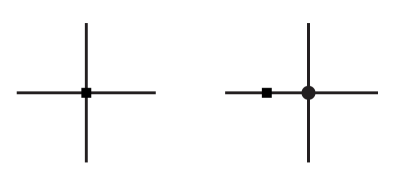
Figure 1: The tree level diagrams for $K\to 3\pi$. A filled square is a vertex from ${\cal L}_{W2}$ or ${\cal L}_{E2}(\Delta S=1)$ and a filled circle from ${\cal L}_{S2}$ or ${\cal L}_{E2}(\Delta S=0)$.

One of the problems in expressing the amplitudes is the various possible choices of masses to express the isospin conserving piece in. The simplest expressions usually follow when using a mixture of the neutral and charged masses and in the part that is obviously isospin violating we can use the neutral and charged masses interchangeably, denoted by $m_{K}^{2}$ and $m_{\pi}^{2}$.

The simplest expressions for the lowest order we have found are

$$M_{0}(s)|_{p^{2}}=i\,\frac{C\,F_{0}^{4}}{F_{\pi}^{3}\,F_{K}}\left(G_{8}-G_{27}\right)\,\frac{1}{3}\,m_{K^{0}}^{2}\,\left(1+\sqrt{3}\,\sin\epsilon\right)\,.$$ (26)

$$M_{1}(s)|_{p^{2}} = i\frac{CF_{0}^{4}}{F_{\pi}^{3}F_{K}}\Bigg{\{}\left(G_{8}-G_{27}\right)\frac{1}{3}m_{K^{0}}^{2}+\frac{\sin\epsilon}{\sqrt{3}}\left(G_{8}-\frac{13}{3}G_{27}\right)m_{K}^{2}$$

$$+Ze^{2}F_{0}^{2}\left(\frac{4}{3}G_{8}+\frac{G_{27}}{3}\frac{6m_{K}^{2}-16m_{\pi}^{2}}{m_{K}^{2}-m_{\pi}^{2}}\right)\Bigg{\}}\,,$$

$$M_{2}(s)|_{p^{2}} = 0\,,$$

$$M_{3}(s)|_{p^{2}} = i\frac{CF_{0}^{4}}{F_{\pi}^{3}F_{K}}\Bigg{\{}-\frac{G_{8}}{3}+G_{27}\left(-\frac{1}{2}+\frac{1}{3}\frac{m_{\pi^{+}}^{2}}{m_{K^{+}}^{2}-m_{\pi^{+}}^{2}}+\frac{1}{2}\frac{m_{\pi^{0}}^{2}}{m_{K^{0}}^{2}-m_{\pi^{0}}^{2}}\right)$$ (27)

$$+\frac{\sin\epsilon}{\sqrt{3}}\left(-2G_{8}+\frac{17}{6}G_{27}\frac{m_{K}^{2}}{m_{K}^{2}-m_{\pi}^{2}}\right)+\left(Z\,G_{8}+\frac{1}{2}G_{E}\right)\frac{e^{2}F_{0}^{2}}{m_{K}^{2}-m_{\pi}^{2}}\Bigg{\}}.$$

$$M_{4}(s)|_{p^{2}} = 0\,,$$

$$M_{5}(s)|_{p^{2}} = 0\,,$$

$$M_{6}(s)|_{p^{2}} = i\frac{CF_{0}^{4}}{F_{\pi}^{3}F_{K}}\Bigg{\{}G_{27}\left(-\frac{5}{2}-\frac{1}{3}\frac{m_{\pi^{+}}^{2}}{m_{K^{+}}^{2}-m_{\pi^{+}}^{2}}-\frac{1}{2}\frac{m_{\pi^{0}}^{2}}{m_{K^{0}}^{2}-m_{\pi^{0}}^{2}}\right)$$ (28)

$$+\frac{\sin\epsilon}{\sqrt{3}}\left(-G_{8}+\frac{G_{27}}{2}\frac{7m_{K}^{2}-6m_{\pi}^{2}}{m_{K}^{2}-m_{\pi}^{2}}\right)+\left(-Z\,G_{8}-\frac{1}{2}G_{E}\right)\frac{e^{2}F_{0}^{2}}{m_{K}^{2}-m_{\pi}^{2}}\Bigg{\}}\,.$$

This is in the isospin limit the same as (31) in [10] using Eq. (A.9) there.

$$M_{7}(s)|_{p^{2}} = i\frac{CF_{0}^{4}}{F_{\pi}^{3}F_{K}}\Bigg{\{}\left(-\frac{1}{3}G_{8}-\frac{2}{9}G_{27}\right)m_{K^{+}}^{2}-\frac{10}{3}\frac{\sin\epsilon}{\sqrt{3}}m_{K}^{2}G_{27}$$

$$+Ze^{2}F_{0}^{2}\left(-\frac{8}{3}G_{8}+\frac{G_{27}}{9}\frac{-46m_{K}^{2}+16m_{\pi}^{2}}{m_{K}^{2}-m_{\pi}^{2}}\right)-G_{E}e^{2}F_{0}^{2}\Bigg{\}}\,,$$

$$M_{8}(s)|_{p^{2}} = 0\,,$$

$$M_{9}(s)|_{p^{2}} = i\frac{CF_{0}^{4}}{F_{\pi}^{3}F_{K}}\Bigg{\{}\frac{G_{8}}{3}+G_{27}\left(\frac{19}{18}+\frac{1}{3}\frac{m_{\pi^{+}}^{2}}{m_{K^{+}}^{2}-m_{\pi^{+}}^{2}}+\frac{1}{2}\frac{m_{\pi^{0}}^{2}}{m_{K^{0}}^{2}-m_{\pi^{0}}^{2}}\right)$$ (29)

$$+\frac{\sin\epsilon}{\sqrt{3}}\left(G_{8}+\frac{G_{27}}{3}\frac{7m_{K}^{2}-6m_{\pi}^{2}}{m_{K}^{2}-m_{\pi}^{2}}\right)+\left(Z\,G_{8}+\frac{1}{2}G_{E}\right)\frac{e^{2}F_{0}^{2}}{m_{K}^{2}-m_{\pi}^{2}}\Bigg{\}}\,.$$

This can be brought into the form of (32) of [10] using the equivalents of (A.3-A.5) there.

$$M_{10}(s)|_{p^{2}} = i\frac{CF_{0}^{4}}{F_{\pi}^{3}F_{K}}\Bigg{\{}G_{8}\left(s-m_{K^{+}}^{2}-m_{\pi^{+}}^{2}\right)+G_{27}\left(-\frac{13}{3}s+m_{K^{+}}^{2}+\frac{13}{3}m_{\pi^{+}}^{2}\right)$$

$$-8Ze^{2}F_{0}^{2}\,G_{8}-\frac{16}{3}Ze^{2}F_{0}^{2}\,G_{27}-2\,G_{E}e^{2}F_{0}^{2}\Bigg{\}}\,,$$

$$M_{11}(s)|_{p^{2}} = 0\,,$$

$$M_{12}(s)|_{p^{2}} = 0\,.$$ (30)

Here $F_{\pi}$ and $F_{K}$ are the pion and kaon decay constants respectively.

The terms proportional to $G_{E}$ are published before in [11] and, after sorting out some misprints there, the results fully agree.

5.2 Next-to-leading order

The results at next-to-leading order are a lot longer, and we decided to not include them all explicitely. $A^{L}_{000}$ is however the full first order isospin breaking amplitude (no explicit photon diagrams contribute) and we therefore present it in App. A. The expressions for the remaining amplitudes are available on request from the authors or can be downloaded [24].

The diagrams contributing are the same as in [10], see figure there. Note however that vertices from ${\cal L}_{W4}$ can now also be from ${\cal L}_{W2E2}$, ${\cal L}_{S4}$ also from ${\cal L}_{S2E2}$ and vertices from ${\cal L}_{S2}$ or ${\cal L}_{W2}$ also from ${\cal L}_{E2}$.

The amplitudes at next-to-leading order can in principle include all the parameters from ${\cal L}_{W4}$, ${\cal L}_{S4}$, ${\cal L}_{W2E2}$ and ${\cal L}_{S2E2}$. The coefficients from the strong and electromagnetic Lagrangians are treated as known, which leaves $G_{8}$,$G_{27}$,$N^{r}_{1},\ldots,N^{r}_{13}$, $D^{r}_{1}$,$D^{r}_{2}$,$D^{r}_{4},\ldots,D^{r}_{7}$, $D^{r}_{26},\ldots,D^{r}_{31}$ and $Z^{r}_{1},\ldots,Z^{r}_{14}$ as unknown. In total 41 undetermined parameters. However, all of these don’t have to be independent in the sense that they multiply the same type of term, eg. $m_{K}^{4}$ or $e^{2}m_{\pi}^{2}$. It turns out that there are 30 independent combinations, denoted by $\tilde{K}_{1}\ldots\tilde{K}_{30}$. See Table 2 for the ones already present in the isospin limit [10] and Table 3 for the new isospin breaking combinations. $\tilde{K}_{12}$ to $\tilde{K}_{19}$ multiply terms including $\sin\epsilon$, $\tilde{K}_{20}$ to $\tilde{K}_{28}$ terms including $e^{2}$ and $\tilde{K}_{29}$ and $\tilde{K}_{30}$ terms including $Ze^{2}$.

The results proportional to $G_{E}$ at next-to-leading order are also published in [11] and, after sorting out some misprints there, the results fully agree.

The corrections to the masses and decay constants including strong isospin breaking were also recalculated, and they were found to agree with the known results, see [20, 23] and references therein.

$\tilde{K}_{1}$	$G_{8}\left(N_{5}^{r}-2N_{7}^{r}+2N_{8}^{r}+N_{9}^{r}\right)+G_{27}\left(-\frac{1}{2}D_{6}^{r}\right)$
$\tilde{K}_{2}$	$G_{8}\left(N_{1}^{r}+N_{2}^{r}\right)+G_{27}\left(\frac{1}{3}D_{26}^{r}-\frac{4}{3}D_{28}^{r}\right)$
$\tilde{K}_{3}$	$G_{8}\left(N_{3}^{r}\right)+G_{27}\left(\frac{2}{3}D_{27}^{r}+\frac{2}{3}D_{28}^{r}\right)$
$\tilde{K}_{4}$	$G_{27}\left(D_{4}^{r}-D_{5}^{r}+4D_{7}^{r}\right)$
$\tilde{K}_{5}$	$G_{27}\left(D_{30}^{r}+D_{31}^{r}+2D_{28}^{r}\right)$
$\tilde{K}_{6}$	$G_{27}\left(8D_{28}^{r}-D_{29}^{r}+D_{30}^{r}\right)$
$\tilde{K}_{7}$	$G_{27}\left(-4D_{28}^{r}+D_{29}^{r}\right)$
$\tilde{K}_{8}$	$G_{8}\left(2N_{5}^{r}+4N_{7}^{r}+N_{8}^{r}-2N_{10}^{r}-4N_{11}^{r}-2N_{12}^{r}\right)+G_{27}\left(-\frac{2}{3}D_{1}^{r}+\frac{2}{3}D_{6}^{r}\right)$
$\tilde{K}_{9}$	$G_{8}\left(N_{5}^{r}+N_{8}^{r}+N_{9}^{r}\right)+G_{27}\left(-\frac{1}{6}D_{6}^{r}\right)$
$\tilde{K}_{10}$	$G_{27}\left(2D_{2}^{r}-2D_{4}^{r}-D_{7}^{r}\right)$
$\tilde{K}_{11}$	$G_{27}\left(D_{7}^{r}\right)$

Table 2: The independent linear combinations of the $N_{i}^{r}$ and $D_{i}^{r}$ that appear in the isospin invariant amplitudes.

$\tilde{K}_{12}$	$G_{8}\left(3\,N_{6}^{r}-4\,N_{9}^{r}-5\,N_{10}^{r}-6\,N_{11}^{r}-7\,N_{12}^{r}-6\,N_{13}^{r}\right)$
	$+G_{27}\left(23/3\,D_{1}^{r}-5/3\,D_{6}^{r}\right)$
$\tilde{K}_{13}$	$G_{27}\left(10/3\,D_{1}^{r}-11/12\,D_{6}^{r}\right)$
$\tilde{K}_{14}$	$G_{27}\left(5\,D_{27}^{r}+5/2\,D_{31}^{r}\right)$
$\tilde{K}_{15}$	$G_{27}\left(-2/3\,D_{26}^{r}-8/3\,D_{27}^{r}\right)$
$\tilde{K}_{16}$	$G_{8}\left(2\,N_{9}^{r}+3\,N_{10}^{r}+4\,N_{11}^{r}+N_{12}^{r}\right)$
	$+G_{27}\left(D_{1}^{r}-1/3\,D_{6}^{r}\right)$
$\tilde{K}_{17}$	$G_{27}\left(D_{6}^{r}\right)$
$\tilde{K}_{18}$	$G_{8}\left(9/2\,N_{4}^{r}\right)+G_{27}\left(-2\,D_{26}^{r}-6\,D_{27}^{r}+D_{31}^{r}\right)$
$\tilde{K}_{19}$	$G_{8}\left(3/2\,N_{2}^{r}\right)+G_{27}\left(3/2\,D_{26}^{r}+4\,D_{27}^{r}-D_{31}^{r}\right)$
$\tilde{K}_{20}$	$G_{8}\left(-3\,Z_{2}^{r}+2\,Z_{3}^{r}-18/5\,Z_{4}^{r}+3/4\,Z_{5}^{r}+1/2\,Z_{6}^{r}+1/2\,Z_{7}^{r}\right.$
	$\left.+3/4\,Z_{8}^{r}+3/4\,Z_{9}^{r}+1/2\,Z_{10}^{r}+7/10\,Z_{11}^{r}+7/10\,Z_{12}^{r}\right)$
$\tilde{K}_{21}$	$G_{8}\left(2\,Z_{8}^{r}+2/3\,Z_{10}^{r}+2/3\,Z_{11}^{r}-2\,Z_{12}^{r}\right)$
$\tilde{K}_{22}$	$G_{8}\left(2\,Z_{6}^{r}+2\,Z_{8}^{r}+2\,Z_{9}^{r}+4/3\,Z_{10}^{r}+2/3\,Z_{11}^{r}+2/3\,Z_{12}^{r}+2\,Z_{13}^{r}+1/3\,Z_{14}^{r}\right)$
$\tilde{K}_{23}$	$G_{8}\left(Z_{12}^{r}\right)$
$\tilde{K}_{24}$	$G_{8}\left(Z_{7}^{r}+3\,Z_{8}^{r}+Z_{10}^{r}+3\,Z_{11}^{r}-Z_{12}^{r}\right)$
$\tilde{K}_{25}$	$G_{8}\left(-4\,Z_{1}^{r}-2\,Z_{2}^{r}-4/3\,Z_{3}^{r}+4\,Z_{4}^{r}-3/2\,Z_{5}^{r}+Z_{6}^{r}\right.$
	$\left.-Z_{7}^{r}+1/2\,Z_{8}^{r}+1/2\,Z_{9}^{r}+1/3\,Z_{10}^{r}-1/3\,Z_{11}^{r}-1/3\,Z_{12}^{r}\right)$
$\tilde{K}_{26}$	$G_{8}\left(-12/5\,Z_{4}^{r}+3/2\,Z_{5}^{r}-Z_{6}^{r}+Z_{7}^{r}-3/2\,Z_{8}^{r}\right.$
	$\left.-3/2\,Z_{9}^{r}-Z_{10}^{r}-1/5\,Z_{11}^{r}-1/5\,Z_{12}^{r}\right)$
$\tilde{K}_{27}$	$G_{8}\left(8/5\,Z_{4}^{r}+4/5\,Z_{11}^{r}+4/5\,Z_{12}^{r}\right)$
$\tilde{K}_{28}$	$G_{8}\left(Z_{3}^{r}+Z_{6}^{r}+3/2\,Z_{8}^{r}+3/2\,Z_{9}^{r}+Z_{10}^{r}+1/2\,Z_{11}^{r}+1/2\,Z_{12}^{r}\right)$
$\tilde{K}_{29}$	$G_{8}\left(3\,N_{10}^{r}+4\,N_{11}^{r}+N_{12}^{r}\right)$
	$+G_{27}\left(D_{1}^{r}+2/3\,D_{5}^{r}-1/3\,D_{6}^{r}\right)$
$\tilde{K}_{30}$	$G_{8}\left(8/3\,N_{11}^{r}+8/3\,N_{12}^{r}\right)+G_{27}\left(16/9\,D_{5}^{r}+4/9\,D_{6}^{r}\right)$

Table 3: The new independent linear combinations of the $N_{i}^{r}$, $D_{i}^{r}$ and $Z_{i}^{r}$ that appear in the isospin breaking amplitudes.

6 Numerical Results

6.1 Experimental data and fit

A full isospin limit fit was made in [10] taking into account all data published before May 2002. One of the reasons for this investigation of isospin breaking effects is to see whether isospin violation can solve the discrepancies in the quadratic slope parameters found there. A new full fit will be done after all the electromagnetic contributions have been included in the amplitudes (work in progress). The data from ISTRA+ [25] and KLOE [26], which appeared after [10], will then also be taken into account.

6.2 Results with and without strong isospin breaking

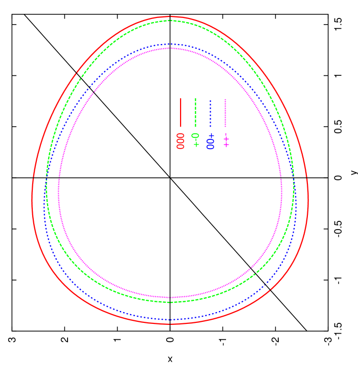
Figure 2: The phase space boundaries for the five different decays and the curves along which we will compare the amplitudes.

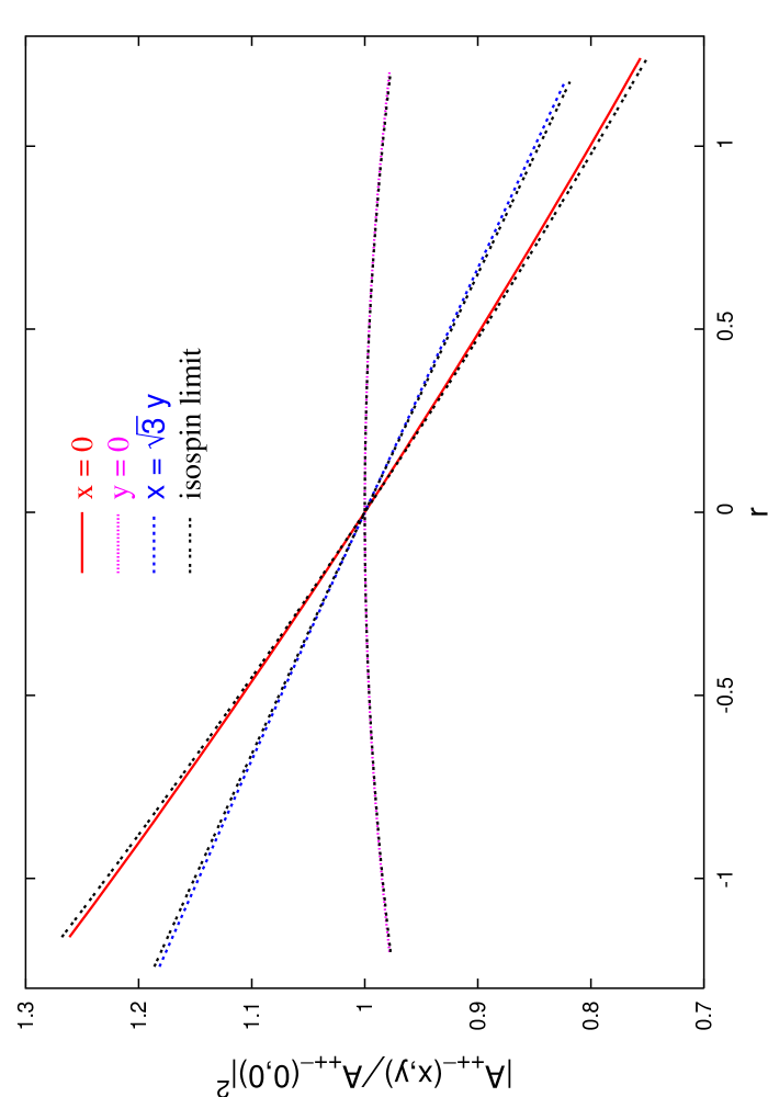
Figure 7: Comparison of $K^{+}\to\pi^{+}\pi^{+}\pi^{-}$ with and without strong isospin breaking.

Our main result is the comparison between the amplitudes in the isospin limit and including first order strong isospin breaking. In Fig. 2 we show the phase space boundaries for the five different decays and the three curves along which we will show results for the squared amplitudes with and without first order strong isospin breaking. The three curves are $x=0$, $y=0$ and $x=\sqrt{3}\,y$. In Fig. 3 to Fig. 7 we then plot the different squared amplitudes along these curves as a function of $r$, where $r=\pm\sqrt{y^{2}+\frac{x^{2}}{3}}$ and the sign is chosen in the natural way,

$$r=\left\{\begin{array}[]{ll}y,&x=0\\ x/\sqrt{3},&y=0\\ y\,\sqrt{2},&x=y\,\sqrt{3}\,.\end{array}\right.$$ (31)

Note that for all but $A^{S}_{+-0}$ the squared amplitudes are normalized to their value at the center of the Dalitz plot. A comparison of the central values themselves is shown in Table 5 together with the decay rates integrated over the Dalitz region. In Fig. 3 one can clearly see the thresholds introduced by the difference between $m^{2}_{\pi^{+}}$ and $m^{2}_{\pi^{0}}$ induced by the breaking of strong isospin invariance. These thresholds correspond to a new process being allowed where two of the neutral pions are produced through an intermediate on shell state with one positive and one negative pion.

$G_{8}$	$5.45$	$L_{1}^{r}$	$0.38\cdot 10^{-3}$	$\tilde{K}_{1}$	$0$
$G_{27}$	$0.392$	$L_{2}^{r}$	$1.59\cdot 10^{-3}$	$\tilde{K}_{2}/G_{8}$	$5.19\cdot 10^{-2}$
$G_{E}$	$-0.4$	$L_{3}^{r}$	$-2.91\cdot 10^{-3}$	$\tilde{K}_{3}/G_{8}$	$3.77\cdot 10^{-3}$
$\delta_{2}-\delta_{0}$	$-0.576$	$L_{4}^{r}$	$0$	$\tilde{K}_{4}$	0
$\sin\epsilon$	$1.19\cdot 10^{-2}$	$L_{5}^{r}$	$1.46\cdot 10^{-3}$	$\tilde{K}_{5}/G_{27}$	$-4.25\cdot 10^{-2}$
$Z$	$0.805$	$L_{6}^{r}$	$0$	$\tilde{K}_{6}/G_{27}$	$-1.66\cdot 10^{-1}$
$\mu$	0.77 GeV	$L_{7}^{r}$	$-0.49\cdot 10^{-3}$	$\tilde{K}_{7}/G_{27}$	$1.20\cdot 10^{-1}$
$F_{\pi}$	$0.0924$ GeV	$L_{8}^{r}$	$1.0\cdot 10^{-3}$	$\tilde{K}_{8}\ldots\tilde{K}_{11}$	0
$F_{K}$	$0.113$ GeV	$K_{1}\ldots K_{11}$	$0$	$\tilde{K}_{12}\ldots\tilde{K}_{30}$	$0$

Table 4: The various input values used.

The input values used to get the results can be seen in Table 4. $L_{1}^{r}$ to $L_{8}^{r}$ come from a one-loop fit in [17], $G_{8}$, $G_{27}$, $\delta_{2}-\delta_{0}$ and $\tilde{K}_{1}$ to $\tilde{K}_{11}$ from the isospin limit fit in [10], $G_{E}$ from [27] and $\sin\epsilon$ from [17]. For $Z$ we use the estimate

$$Z=\frac{1}{2\,F_{\pi}^{2}\,e^{2}}\,(m_{\pi^{+}}^{2}-m_{\pi^{0}}^{2}),$$ (32)

which corresponds to the value in Table 4. As usual, $\mu$ is chosen to be $0.77$ GeV.

Very little knowledge exists of the values of $K_{1}\ldots K_{11}$ and $\tilde{K}_{12}\ldots\tilde{K}_{30}$, so they are set equal to zero (tests were also made assigning order of magnitude estimates to them).

	Centralvalue		Decay Rate
	Isospin limit [10]	Strong iso-br	Isospin limit [10]	Strong iso-br
$K_{L}\to\pi^{0}\pi^{0}\pi^{0}$	$6.74\cdot 10^{-12}$	$6.97\cdot 10^{-12}$	$2.65\cdot 10^{-18}$	$2.74\cdot 10^{-18}$
$K_{L}\to\pi^{+}\pi^{-}\pi^{0}$	$7.46\cdot 10^{-13}$	$7.66\cdot 10^{-13}$	$1.63\cdot 10^{-18}$	$1.67\cdot 10^{-18}$
$K_{S}\to\pi^{+}\pi^{-}\pi^{0}$	$0$	$0$	$3.1\cdot 10^{-21}$	$3.2\cdot 10^{-21}$
$K^{+}\to\pi^{0}\pi^{0}\pi^{+}$	$9.33\cdot 10^{-13}$	$1.01\cdot 10^{-12}$	$9.11\cdot 10^{-19}$	$9.84\cdot 10^{-19}$
$K^{+}\to\pi^{+}\pi^{+}\pi^{-}$	$3.72\cdot 10^{-12}$	$4.00\cdot 10^{-12}$	$2.97\cdot 10^{-18}$	$3.19\cdot 10^{-18}$

Table 5: Comparison of the central values of the amplitudes squared and the decay rates.

There are various ways to treat the masses, especially in the isospin limit case. In [10] the masses used in the phase space were the physical masses occuring in the decays. However in the amplitudes the physical kaon mass of the kaon involved in the process was used and the pion mass was given by $m_{\pi}^{2}=\frac{1}{3}\sum_{i=1,3}m_{\pi^{i}}^{2}$ with $i=1,2,3$ being the three pions participating in the reaction. This allowed for the correct kinematical relation $s_{1}+s_{2}+s_{3}=m_{K}^{2}+3m_{\pi}^{2}$ to be satisfied while having the isospin limit in the amplitude but the physical masses in the phase space. The results presented used the Gell-Mann-Okubo (GMO) relation for the eta mass in the loops. Results with the physical eta mass gave small changes within the general errors given in [10]. In the present isospin breaking calculation all the pion and kaon masses were used correctly in the amplitude, but for the eta we again use the GMO relation, but now including isospin breaking,

$$m_{\eta}^{2}=\frac{2}{3}\,(m_{K^{+}}^{2}+m_{K^{0}}^{2}-m_{\pi^{+}}^{2})+\frac{1}{3}\,m_{\pi^{0}}^{2}\,.$$ (33)

The possible lowest order contributions from the eta mass have been removed from the amplitudes using the corresponding next-to-leading order relation.

Here follows a discussion of the results in somewhat more detail. In general the results are of a size as can be expected from this type of isospin breaking. They are of order a few, up to 5% in the amplitudes. The isospin breaking corrections tend to increase all decay rates somewhat but this can be compensated by small changes in the values of the fitted $\tilde{K}_{i}$ compared to the results of [10]. The number of significant digits quoted in Table 5 is higher than the expected precision of our results, but the trend and the general size of the change compared to the isospin conserving results are stable with respect to variations in dealing with the eta mass (physical or GMO).

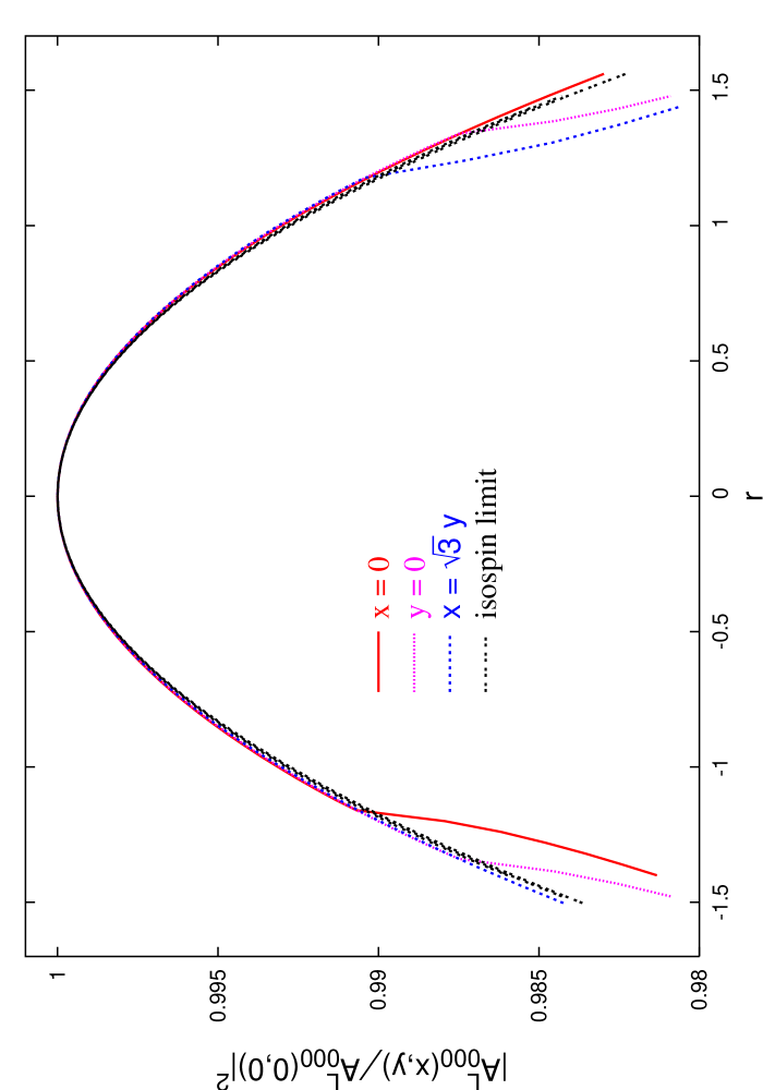
Figure 3: Comparison of $K_{L}\to\pi^{0}\pi^{0}\pi^{0}$ with and without strong isospin breaking.

For $K_{L}\to\pi^{0}\pi^{0}\pi^{0}$ the central value of the amplitude squared increases by about 3%. The change in the quadratic slope is similar but the total variation over the Dalitz plot is small so the total decay rate increases by about 3% as well. This decay is the one which has most variation in the amplitude when changing how one deals with the eta mass. The extreme case we have found was that this effect completely cancelled the change from isospin violation. For this decay the amplitude as presented in the paper is also the final one. There are no contributions from loops with photons for this decay. It will only be indirectly affected when the $\tilde{K}_{i}$ are determined from the decays involving charged particles which do have contributions from loops and tree level diagrams with photons. Note the scale in Fig. 3 when viewing the result.

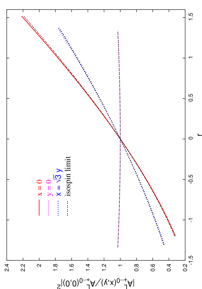
Figure 4: Comparison of $K_{L}\to\pi^{+}\pi^{-}\pi^{0}$ with and without strong isospin breaking.

The squared amplitude $K_{L}\to\pi^{+}\pi^{-}\pi^{0}$ increases by about 2.5% with very little variation with the eta mass treatment. The decay rate increases by the same amount. The changes in the Dalitz plot slopes are similar as can be judged from Fig. 4.

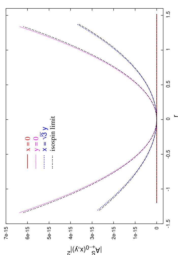
Figure 5: Comparison of $K_{S}\to\pi^{+}\pi^{-}\pi^{0}$ with and without strong isospin breaking.

For the decay $K_{S}\to\pi^{+}\pi^{-}\pi^{0}$ the amplitude in the center of the Dalitz plot vanishes because of the symmetries. The amplitude and the slopes increase by about 3% as can be seen in Fig. 5.

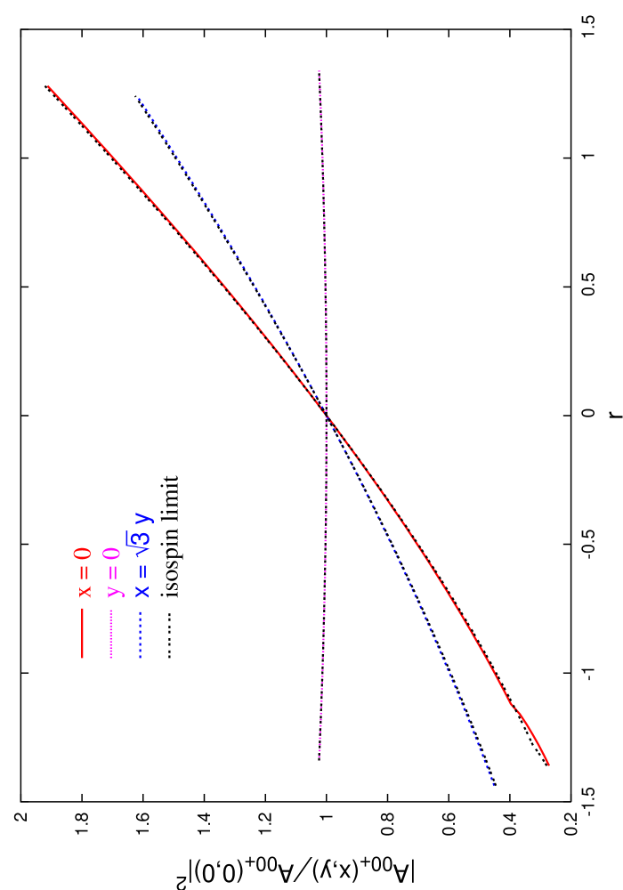
Figure 6: Comparison of $K^{+}\to\pi^{0}\pi^{0}\pi^{+}$ with and without strong isospin breaking.

The decay $K^{+}\to\pi^{0}\pi^{0}\pi^{+}$ has the largest increase. The squared amplitude in the center changes by about 11%. The linear slopes decrease somewhat leading to an increase of about 8% to the total decay rate when compared with the isospin conserved case.

The decay $K^{+}\to\pi^{+}\pi^{+}\pi^{-}$ has a change of about 7.5% upwards in the center of the Dalitz plot and a similar change in the decay rate. The slopes decrease somewhat.

The conclusions above do not seem to change qualitatively when we give the $K_{i}^{r}$ a value of about $0.001$ and the extra $\tilde{K}_{i}$ a value relative to $G_{8}$ and $G_{27}$ of $0.01$. However the changes induced by these values can be of the order of 10%, largest for $K_{L}\to\pi^{0}\pi^{0}\pi^{0}$.

It should be noted that the mentioned changes are with the values of $\tilde{K}_{i}$ determined using the isospin conserving fit. A new determination including isospin breaking effects is planned when the diagrams with photon propagators, both at tree level and one-loop level, have been taken into account. At present most of the changes found can probably be compensated by changes in the $\tilde{K}_{i}$.

7 Conclusions

We have calculated the $K\to 3\pi$ amplitudes to next-to-leading order ($p^{4},p^{2}\,m^{2},m^{4},p^{2}\,e^{2}$) in Chiral Perturbation Theory. A similar calculation was done in [10] in the isospin limit, but we have now included strong isospin breaking ($m_{u}\neq m_{d}$) and local electromagnetic isospin breaking in the amplitudes . This was done partly because it is interesting in general to see the possible importance of isospin breaking in this process, but also to investigate whether isospin violation will improve the fit to experimental data. Discrepancies between data and the quadratic slopes from CHPT were found in [10], and isospin breaking may be the cause of this.

We have tried to estimate the effects of the breaking by comparing the squared amplitudes with and without isospin violation. The effect seems to be at a few percent level, and probably not quite enough to solve the dicrepancies. However, to really investigate this a new full fit has to be done also including the explicit photon diagrams and the new data [25, 26] published after [10]. This is work in progress and will be presented in the future papers Isospin Breaking in $K\to 3\pi$ Decays II and III.

Appendix A The amplitude for $K_{L}\to\pi^{0}\pi^{0}\pi^{0}$.

We divide the $M_{0}(s)$ function defined in Eq. (4) as

$$M_{0}(s) = \left.M_{0}(s)\right|_{p^{2}}+i\frac{CF_{0}^{4}}{F_{\pi}^{3}F_{K}}\left\{\frac{G_{8}}{F_{\pi}^{2}}M_{0}^{8,F}(s)+\frac{G_{8}}{F_{\pi}^{2}}\,\frac{\sin\epsilon}{\sqrt{3}}M_{0}^{8,\epsilon}(s)+G_{8}\,e^{2}M_{0}^{8,e}(s)\right.$$ (A.1)

$$+ \left.\frac{G_{8}^{\prime}}{F_{\pi}^{2}}M_{0}^{8\prime}(s)+\frac{G_{27}}{F_{\pi}^{2}}M_{0}^{27,F}(s)+\frac{G_{27}}{F_{\pi}^{2}}\,\frac{\sin\epsilon}{\sqrt{3}}M_{0}^{27,\epsilon}(s)+G_{27}\,e^{2}M_{0}^{27,e}(s)\right\}\,.$$

The effect of $G_{8}^{\prime}$ cannot be distinguished from higher order coefficients in decays not involving external fields. This was known at tree level earlier and has been proven to one-loop in [5]. This means that terms proportinal to $G_{8}^{\prime}$ are effectively removed.

We have extensively used the first order isospin broken GMO relation,

$$m_{\eta}^{2}=\frac{2}{3}\,(m_{K^{+}}^{2}+m_{K^{0}}^{2}-m_{\pi^{+}}^{2})+\frac{1}{3}\,m_{\pi^{0}}^{2}\,,$$ (A.2)

in writing the amplitude in the form below.

The explicit expressions for $\overline{A}$, $\overline{B}$ and $\overline{B}_{1}$, the finite part of the loop functions, can be found in many places, e.g. [29].

The octet ones are:

$$M^{8,F}_{0}(s)=$$

$$\Big{(}2\,L^{r}_{1}+2\,L^{r}_{2}+L^{r}_{3}\Big{)}\,\Big{(}-8\,m_{\pi^{0}}^{4}-8/3\,m_{K^{0}}^{4}+8\,s^{2}\Big{)}+\Big{(}4\,L^{r}_{4}+L^{r}_{5}\Big{)}\,\Big{(}-8/3\,m_{\pi^{0}}^{2}\,m_{K^{0}}^{2}\Big{)}$$

$$+\Big{(}N^{r}_{1}+N^{r}_{2}+2\,N^{r}_{3}\Big{)}\,\Big{(}m_{\pi^{0}}^{4}+1/3\,m_{K^{0}}^{4}-s^{2}\Big{)}+N^{r}_{5}\,\Big{(}10/3\,m_{\pi^{0}}^{2}\,m_{K^{0}}^{2}+2/3\,m_{K^{0}}^{4}\Big{)}$$

$$+N^{r}_{7}\,\Big{(}4\,m_{\pi^{0}}^{2}\,m_{K^{0}}^{2}-4/3\,m_{K^{0}}^{4}\Big{)}+N^{r}_{8}\,\Big{(}10/3\,m_{\pi^{0}}^{2}\,m_{K^{0}}^{2}+4/3\,m_{K^{0}}^{4}\Big{)}$$

$$+N^{r}_{9}\,\Big{(}-2/3\,m_{\pi^{0}}^{2}\,m_{K^{0}}^{2}+2/3\,m_{K^{0}}^{4}\Big{)}+\Big{(}N^{r}_{10}+2\,N^{r}_{11}+N^{r}_{12}\Big{)}\,\Big{(}-4\,m_{\pi^{0}}^{2}\,m_{K^{0}}^{2}\Big{)}$$

$$+\Big{(}\overline{A}(m_{K^{0}}^{2})-\overline{A}(m_{K^{+}}^{2})\Big{)}\left(\frac{1/4\,m_{\pi}^{4}}{m_{\pi}^{2}-m_{K}^{2}}\right)$$

$$+\overline{A}(m_{\pi^{+}}^{2})\,\Big{(}1/4\,m_{\pi^{0}}^{2}-1/2\,m_{K^{0}}^{2}\Big{)}+\overline{A}(m_{\pi^{0}}^{2})\,\Big{(}17/24\,m_{K^{0}}^{2}\Big{)}$$

$$+\overline{A}(m_{K^{+}}^{2})\,\Big{(}5/36\,m_{\pi^{0}}^{2}+25/36\,m_{K^{0}}^{2}\Big{)}+\overline{A}(m_{K^{0}}^{2})\,\Big{(}-7/18\,m_{\pi^{0}}^{2}-1/36\,m_{K^{0}}^{2}\Big{)}$$

$$+\Big{(}\overline{A}(m_{K^{0}}^{2})-\overline{A}(m_{K^{+}}^{2})\Big{)}\,\Big{(}5/36\,m_{\pi}^{2}+5/18\,m_{K}^{2}\Big{)}+\overline{A}(m_{\eta}^{2})\,\Big{(}1/8\,m_{K^{0}}^{2}\Big{)}$$

$$+\overline{B}(m_{\pi^{+}}^{2},m_{\pi^{+}}^{2},s)\,\Big{(}-2\,m_{\pi^{0}}^{2}\,s+m_{\pi^{0}}^{4}+s^{2}\Big{)}+\overline{B}(m_{\pi^{+}}^{2},m_{K^{+}}^{2},s)\,\Big{(}5/4\,m_{\pi^{0}}^{2}\,m_{K^{0}}^{2}$$

$$~{}~{}-5/4\,m_{\pi^{0}}^{2}\,s-1/2\,m_{K^{0}}^{2}\,s-1/4\,m_{K^{0}}^{4}+3/4\,s^{2}\Big{)}$$

$$+\overline{B}(m_{\pi^{0}}^{2},m_{\pi^{0}}^{2},s)\,\Big{(}1/2\,m_{\pi^{0}}^{2}\,m_{K^{0}}^{2}\Big{)}$$

$$+\overline{B}(m_{\pi^{0}}^{2},m_{K^{0}}^{2},s)\,\Big{(}3/8\,m_{\pi^{0}}^{2}\,m_{K^{0}}^{2}-1/8\,m_{K^{0}}^{2}\,s+1/8\,m_{K^{0}}^{4}\Big{)}$$

$$+\overline{B}(m_{K^{+}}^{2},m_{K^{+}}^{2},s)\,\Big{(}1/4\,m_{\pi^{0}}^{2}\,s+1/4\,m_{K^{0}}^{2}\,s-1/4\,s^{2}\Big{)}$$

$$+\overline{B}(m_{K^{0}}^{2},m_{\eta}^{2},s)\,\Big{(}1/24\,m_{\pi^{0}}^{2}\,m_{K^{0}}^{2}+1/8\,m_{K^{0}}^{2}\,s-5/24\,m_{K^{0}}^{4}\Big{)}$$

$$+\overline{B}(m_{\eta}^{2},m_{\eta}^{2},s)\,\Big{(}1/18\,m_{\pi^{0}}^{2}\,m_{K^{0}}^{2}\Big{)}+\overline{B}_{1}(m_{\pi^{+}}^{2},m_{K^{+}}^{2},s)\,\Big{(}-1/2\,m_{\pi^{0}}^{2}\,m_{K^{0}}^{2}+1/2\,m_{\pi^{0}}^{4}\Big{)}$$

$$+\overline{B}_{1}(m_{\pi^{0}}^{2},m_{K^{0}}^{2},s)\,\Big{(}-1/4\,m_{\pi^{0}}^{2}\,m_{K^{0}}^{2}+1/4\,m_{K^{0}}^{4}\Big{)}$$

$$+\overline{B}_{1}(m_{K^{0}}^{2},m_{\eta}^{2},s)\,\Big{(}-1/4\,m_{\pi^{0}}^{2}\,m_{K^{0}}^{2}+1/4\,m_{K^{0}}^{4}\Big{)}$$

$$M^{8,\epsilon}_{0}(s)=$$

$$\Big{(}2\,L^{r}_{1}+2\,L^{r}_{2}+L^{r}_{3}\Big{)}\,\Big{(}-8\,m_{\pi}^{4}-8/3\,m_{K}^{4}+8\,s^{2}\Big{)}+L^{r}_{4}\,\Big{(}-32/3\,m_{\pi}^{2}\,m_{K}^{2}\Big{)}$$

$$+L^{r}_{5}\,\Big{(}-40/3\,m_{\pi}^{2}\,m_{K}^{2}+16/3\,m_{K}^{4}\Big{)}+L^{r}_{7}\,\Big{(}480\,m_{\pi}^{2}\,m_{K}^{2}-352\,m_{K}^{4}\Big{)}$$

$$+L^{r}_{8}\,\Big{(}224\,m_{\pi}^{2}\,m_{K}^{2}-160\,m_{K}^{4}\Big{)}$$

$$+\Big{(}N^{r}_{1}+N^{r}_{2}-2\,N^{r}_{3}+6\,N^{r}_{4}\Big{)}\,\Big{(}-m_{\pi}^{4}-1/3\,m_{K}^{4}+s^{2}\Big{)}+N^{r}_{5}\,\Big{(}-26/3\,m_{\pi}^{2}\,m_{K}^{2}+10\,m_{K}^{4}\Big{)}$$

$$+N^{r}_{6}\,\Big{(}-48\,m_{\pi}^{2}\,m_{K}^{2}+40\,m_{K}^{4}\Big{)}+N^{r}_{7}\,\Big{(}4\,m_{\pi}^{2}\,m_{K}^{2}-4/3\,m_{K}^{4}\Big{)}$$

$$+N^{r}_{8}\,\Big{(}22/3\,m_{\pi}^{2}\,m_{K}^{2}+4/3\,m_{K}^{4}\Big{)}+N^{r}_{9}\,\Big{(}10/3\,m_{\pi}^{2}\,m_{K}^{2}-10/3\,m_{K}^{4}\Big{)}$$

$$+N^{r}_{10}\,\Big{(}20\,m_{\pi}^{2}\,m_{K}^{2}-16\,m_{K}^{4}\Big{)}+N^{r}_{11}\,\Big{(}-8\,m_{\pi}^{2}\,m_{K}^{2}\Big{)}$$

$$+N^{r}_{12}\,\Big{(}68\,m_{\pi}^{2}\,m_{K}^{2}-64\,m_{K}^{4}\Big{)}+N^{r}_{13}\,\Big{(}96\,m_{\pi}^{2}\,m_{K}^{2}-80\,m_{K}^{4}\Big{)}$$

$$+\frac{1}{m_{\pi}^{2}-m_{K}^{2}}\,\Big{(}\overline{A}(m_{\pi}^{2})-\overline{A}(m_{K}^{2})\Big{)}\,\Big{(}m_{\pi}^{4}\Big{)}+\overline{A}(m_{\pi}^{2})\,\Big{(}-m_{\pi}^{2}+13/8\,m_{K}^{2}\Big{)}$$

$$+\overline{A}(m_{K}^{2})\,\Big{(}m_{\pi}^{2}+3/4\,m_{K}^{2}\Big{)}+\overline{A}(m_{\eta}^{2})\,\Big{(}5/8\,m_{K}^{2}\Big{)}$$

$$+\overline{B}(m_{\pi}^{2},m_{\pi}^{2},s)\,\Big{(}5/2\,m_{\pi}^{2}\,m_{K}^{2}-12\,m_{\pi}^{2}\,s+6\,m_{\pi}^{4}-m_{K}^{2}\,s+6\,s^{2}\Big{)}$$

$$+\overline{B}(m_{\pi}^{2},m_{K}^{2},s)\,\Big{(}-23/8\,m_{\pi}^{2}\,m_{K}^{2}-7\,m_{\pi}^{2}\,s+5\,m_{\pi}^{4}-3/8\,m_{K}^{2}\,s+27/8\,m_{K}^{4}+3\,s^{2}\Big{)}$$

$$+\overline{B}(m_{\pi}^{2},m_{\eta}^{2},s)\,\Big{(}4/3\,m_{\pi}^{2}\,m_{K}^{2}-4/3\,m_{K}^{4}\Big{)}$$

$$+\overline{B}(m_{K}^{2},m_{K}^{2},s)\,\Big{(}-2\,m_{\pi}^{2}\,m_{K}^{2}+3\,m_{\pi}^{2}\,s+4\,m_{K}^{2}\,s-2\,m_{K}^{4}-3\,s^{2}\Big{)}$$

$$+\overline{B}(m_{K}^{2},m_{\eta}^{2},s)\,\Big{(}-11/24\,m_{\pi}^{2}\,m_{K}^{2}-3/8\,m_{K}^{2}\,s+23/24\,m_{K}^{4}\Big{)}$$

$$+\overline{B}(m_{\eta}^{2},m_{\eta}^{2},s)\,\Big{(}-5/18\,m_{\pi}^{2}\,m_{K}^{2}\Big{)}+\overline{B}_{1}(m_{\pi}^{2},m_{K}^{2},s)\,\Big{(}5/4\,m_{\pi}^{2}\,m_{K}^{2}-5/4\,m_{K}^{4}\Big{)}$$

$$+\overline{B}_{1}(m_{K}^{2},m_{\eta}^{2},s)\,\Big{(}3/4\,m_{\pi}^{2}\,m_{K}^{2}-3/4\,m_{K}^{4}\Big{)}$$

$$M^{8,e}_{0}(s)=$$

$$\Big{(}3\,Z^{r}_{5}-2\,Z^{r}_{6}+2\,Z^{r}_{7}-3\,Z^{r}_{8}-3\,Z^{r}_{9}-2\,Z^{r}_{10}+2\,Z^{r}_{11}+2\,Z^{r}_{12}\Big{)}\Big{(}1/9\,m_{K}^{2}\Big{)}$$

$$\Big{(}-2\,K^{r}_{3}+K^{r}_{4}\Big{)}\,\Big{(}1/2\,m_{\pi}^{2}-m_{K}^{2}\Big{)}+\Big{(}K^{r}_{5}+K^{r}_{6}\Big{)}\,\Big{(}1/3\,m_{\pi}^{2}+2/9\,m_{K}^{2}\Big{)}$$

$$+\Big{(}K^{r}_{9}+K^{r}_{10}\Big{)}\,\Big{(}-1/3\,m_{\pi}^{2}\Big{)}+K^{r}_{12}\,\Big{(}8/3\,m_{K}^{2}\Big{)}$$

$$+\frac{m_{\pi}^{4}}{m_{\pi}^{2}-m_{K}^{2}}\,\Big{(}K^{r}_{3}-1/2\,K^{r}_{4}-1/3\,K^{r}_{5}-1/3\,K^{r}_{6}+1/3\,K^{r}_{9}+1/3\,K^{r}_{10}\Big{)}$$

$$+\frac{1}{m_{\pi}^{2}-m_{K}^{2}}\,\Big{(}\overline{A}(m_{\pi}^{2})-\overline{A}(m_{K}^{2})\Big{)}\,\Big{(}-m_{\pi}^{2}\,Z-1/2\,m_{\pi}^{2}\,\frac{G_{E}}{G_{8}}\Big{)}$$

$$+\frac{1}{m_{\pi}^{2}-m_{K}^{2}}\,\overline{B}(m_{\pi}^{2},m_{\pi}^{2},s)\,\Big{(}-7\,m_{\pi}^{2}\,Z\,s-7/2\,m_{\pi}^{2}\,\frac{G_{E}}{G_{8}}\,s$$

$$~{}~{}+4\,m_{\pi}^{4}\,Z+2\,m_{\pi}^{4}\,\frac{G_{E}}{G_{8}}+3\,Z\,s^{2}+3/2\,\frac{G_{E}}{G_{8}}\,s^{2}\Big{)}$$

$$+\frac{1}{m_{\pi}^{2}-m_{K}^{2}}\,\overline{B}(m_{\pi}^{2},m_{K}^{2},s)\,\Big{(}6\,m_{\pi}^{2}\,Z\,s+3\,m_{\pi}^{2}\,\frac{G_{E}}{G_{8}}\,s-4\,m_{\pi}^{4}\,Z$$

$$~{}~{}-2\,m_{\pi}^{4}\,\frac{G_{E}}{G_{8}}-9/4\,Z\,s^{2}-9/8\,\frac{G_{E}}{G_{8}}\,s^{2}\Big{)}$$

$$+\frac{1}{m_{\pi}^{2}-m_{K}^{2}}\,\overline{B}(m_{K}^{2},m_{K}^{2},s)\,\Big{(}m_{\pi}^{2}\,Z\,s+1/2\,m_{\pi}^{2}\,\frac{G_{E}}{G_{8}}\,s-3/4\,Z\,s^{2}-3/8\,\frac{G_{E}}{G_{8}}\,s^{2}\Big{)}$$

$$+\Big{(}\overline{A}(m_{\pi}^{2})-\overline{A}(m_{K}^{2})\Big{)}\,\Big{(}-1/4\,Z-1/8\,\frac{G_{E}}{G_{8}}\Big{)}$$

$$+\overline{B}(m_{\pi}^{2},m_{\pi}^{2},s)\,\Big{(}-m_{\pi}^{2}\,Z-1/2\,m_{\pi}^{2}\,\frac{G_{E}}{G_{8}}+Z\,s+1/2\,\frac{G_{E}}{G_{8}}\,s\Big{)}$$

$$+\overline{B}(m_{\pi}^{2},m_{K}^{2},s)\,\Big{(}7/2\,m_{\pi}^{2}\,Z+7/4\,m_{\pi}^{2}\,\frac{G_{E}}{G_{8}}-3/2\,m_{K}^{2}\,Z-3/4\,m_{K}^{2}\,\frac{G_{E}}{G_{8}}$$

$$~{}~{}-3/4\,Z\,s-3/8\,\frac{G_{E}}{G_{8}}\,s\Big{)}+\overline{B}(m_{K}^{2},m_{K}^{2},s)\,\Big{(}-1/4\,Z\,s-1/8\,\frac{G_{E}}{G_{8}}\,s\Big{)}$$

$$+\overline{B}_{1}(m_{\pi}^{2},m_{K}^{2},s)\,\Big{(}-5/2\,m_{\pi}^{2}\,Z-5/4\,m_{\pi}^{2}\,\frac{G_{E}}{G_{8}}+1/2\,m_{K}^{2}\,Z+1/4\,m_{K}^{2}\,\frac{G_{E}}{G_{8}}\Big{)}$$

And the 27-plets are:

$$M^{27,F}_{0}(s)=$$

$$\Big{(}2\,L^{r}_{1}+2\,L^{r}_{2}+L^{r}_{3}\Big{)}\,\Big{(}8\,m_{\pi^{0}}^{4}+8/3\,m_{K^{0}}^{4}-8\,s^{2}\Big{)}+\Big{(}4\,L^{r}_{4}+L^{r}_{5}\Big{)}\,\Big{(}8/3\,m_{\pi^{0}}^{2}\,m_{K^{0}}^{2}\Big{)}$$

$$+\Big{(}D^{r}_{1}-3\,D^{r}_{2}\Big{)}\,\Big{(}-4/3\,m_{\pi^{0}}^{2}\,m_{K^{0}}^{2}\Big{)}+D^{r}_{4}\,\Big{(}-11/3\,m_{\pi^{0}}^{2}\,m_{K^{0}}^{2}-1/3\,m_{K^{0}}^{4}\Big{)}$$

$$+D^{r}_{5}\,\Big{(}-1/3\,m_{\pi^{0}}^{2}\,m_{K^{0}}^{2}+1/3\,m_{K^{0}}^{4}\Big{)}+D^{r}_{6}\,\Big{(}7/9\,m_{\pi^{0}}^{2}\,m_{K^{0}}^{2}-1/3\,m_{K^{0}}^{4}\Big{)}$$

$$+D^{r}_{7}\,\Big{(}-10/3\,m_{\pi^{0}}^{2}\,m_{K^{0}}^{2}-4/3\,m_{K^{0}}^{4}\Big{)}$$

$$+\Big{(}D^{r}_{26}+4\,D^{r}_{27}-3\,D^{r}_{29}-6\,D^{r}_{30}-6\,D^{r}_{31}\Big{)}\,\Big{(}1/3\,m_{\pi^{0}}^{4}+1/9\,m_{K^{0}}^{4}-1/3\,s^{2}\Big{)}$$

$$+\frac{1}{m_{\pi}^{2}-m_{K}^{2}}\,\Big{(}\overline{A}(m_{K^{0}}^{2})-\overline{A}(m_{K^{+}}^{2})\Big{)}\,\Big{(}7/12\,m_{\pi}^{4}\Big{)}$$

$$+\frac{1}{m_{\pi^{0}}^{2}-m_{K^{0}}^{2}}\,\overline{A}(m_{\pi^{+}}^{2})\,\Big{(}-5/6\,m_{\pi^{0}}^{4}\Big{)}+\frac{1}{m_{\pi^{0}}^{2}-m_{K^{0}}^{2}}\,\overline{A}(m_{K^{+}}^{2})\,\Big{(}5/3\,m_{\pi^{0}}^{4}\Big{)}$$

$$+\frac{1}{m_{\pi^{0}}^{2}-m_{K^{0}}^{2}}\,\overline{A}(m_{K^{0}}^{2})\,\Big{(}-5/6\,m_{\pi^{0}}^{4}\Big{)}$$

$$+\frac{1}{m_{\pi^{0}}^{2}-m_{K^{0}}^{2}}\,\overline{B}(m_{\pi^{+}}^{2},m_{\pi^{+}}^{2},s)\,\Big{(}5/2\,m_{\pi^{0}}^{2}\,s^{2}-35/6\,m_{\pi^{0}}^{4}\,s+10/3\,m_{\pi^{0}}^{6}\Big{)}$$

$$+\frac{1}{m_{\pi^{0}}^{2}-m_{K^{0}}^{2}}\,\overline{B}(m_{\pi^{+}}^{2},m_{K^{+}}^{2},s)\,\Big{(}-15/8\,m_{\pi^{0}}^{2}\,s^{2}+5\,m_{\pi^{0}}^{4}\,s-10/3\,m_{\pi^{0}}^{6}\Big{)}$$

$$+\frac{1}{m_{\pi^{0}}^{2}-m_{K^{0}}^{2}}\,\overline{B}(m_{K^{+}}^{2},m_{K^{+}}^{2},s)\,\Big{(}-5/8\,m_{\pi^{0}}^{2}\,s^{2}+5/6\,m_{\pi^{0}}^{4}\,s\Big{)}$$

$$+\overline{A}(m_{\pi^{+}}^{2})\,\Big{(}m_{\pi^{0}}^{2}-109/72\,m_{K^{0}}^{2}\Big{)}+\overline{A}(m_{\pi^{0}}^{2})\,\Big{(}-17/24\,m_{K^{0}}^{2}\Big{)}$$

$$+\overline{A}(m_{K^{+}}^{2})\,\Big{(}-25/18\,m_{\pi^{0}}^{2}-25/72\,m_{K^{0}}^{2}\Big{)}+\overline{A}(m_{K^{0}}^{2})\,\Big{(}7/18\,m_{\pi^{0}}^{2}+1/36\,m_{K^{0}}^{2}\Big{)}$$

$$+\Big{(}\overline{A}(m_{K^{0}}^{2})-\overline{A}(m_{K^{+}}^{2})\Big{)}\,\Big{(}-5/36\,m_{\pi}^{2}-5/18\,m_{K}^{2}\Big{)}+\overline{A}(m_{\eta}^{2})\,\Big{(}-1/8\,m_{K^{0}}^{2}\Big{)}$$

$$+\overline{B}(m_{\pi^{+}}^{2},m_{\pi^{+}}^{2},s)\,\Big{(}5/6\,m_{\pi^{0}}^{2}\,m_{K^{0}}^{2}-13/6\,m_{\pi^{0}}^{2}\,s+2/3\,m_{\pi^{0}}^{4}$$

$$~{}~{}-5/6\,m_{K^{0}}^{2}\,s+3/2\,s^{2}\Big{)}$$

$$+\overline{B}(m_{\pi^{+}}^{2},m_{K^{+}}^{2},s)\,\Big{(}25/6\,m_{\pi^{0}}^{2}\,m_{K^{0}}^{2}-35/6\,m_{\pi^{0}}^{2}\,s+10/3\,m_{\pi^{0}}^{4}$$

$$~{}~{}-53/24\,m_{K^{0}}^{2}\,s-1/6\,m_{K^{0}}^{4}+19/8\,s^{2}\Big{)}$$

$$+\overline{B}(m_{\pi^{0}}^{2},m_{\pi^{0}}^{2},s)\,\Big{(}-1/2\,m_{\pi^{0}}^{2}\,m_{K^{0}}^{2}\Big{)}$$

$$+\overline{B}(m_{\pi^{0}}^{2},m_{K^{0}}^{2},s)\,\Big{(}-3/8\,m_{\pi^{0}}^{2}\,m_{K^{0}}^{2}+1/8\,m_{K^{0}}^{2}\,s-1/8\,m_{K^{0}}^{4}\Big{)}$$

$$+\overline{B}(m_{K^{+}}^{2},m_{K^{+}}^{2},s)\,\Big{(}-13/12\,m_{\pi^{0}}^{2}\,s-7/8\,m_{K^{0}}^{2}\,s+7/8\,s^{2}\Big{)}$$

$$+\overline{B}(m_{K^{0}}^{2},m_{\eta}^{2},s)\,\Big{(}-1/24\,m_{\pi^{0}}^{2}\,m_{K^{0}}^{2}-1/8\,m_{K^{0}}^{2}\,s+5/24\,m_{K^{0}}^{4}\Big{)}$$

$$+\overline{B}(m_{\eta}^{2},m_{\eta}^{2},s)\,\Big{(}-1/18\,m_{\pi^{0}}^{2}\,m_{K^{0}}^{2}\Big{)}$$

$$+\overline{B}_{1}(m_{\pi^{+}}^{2},m_{K^{+}}^{2},s)\,\Big{(}-19/12\,m_{\pi^{0}}^{2}\,m_{K^{0}}^{2}+1/3\,m_{\pi^{0}}^{4}-5/12\,m_{K^{0}}^{4}\Big{)}$$

$$+\Big{(}\overline{B}_{1}(m_{\pi^{0}}^{2},m_{K^{0}}^{2},s)+\overline{B}_{1}(m_{K^{0}}^{2},m_{\eta}^{2},s)\Big{)}\,\Big{(}1/4\,m_{\pi^{0}}^{2}\,m_{K^{0}}^{2}-1/4\,m_{K^{0}}^{4}\Big{)}$$

$$M^{27,\epsilon}_{0}(s)=$$

$$\Big{(}2\,L^{r}_{1}+2\,L^{r}_{2}+L^{r}_{3}\Big{)}\,\Big{(}8\,m_{\pi}^{4}+8/3\,m_{K}^{4}-8\,s^{2}\Big{)}$$

$$+L^{r}_{4}\,\Big{(}32/3\,m_{\pi}^{2}\,m_{K}^{2}\Big{)}+L^{r}_{5}\,\Big{(}40/3\,m_{\pi}^{2}\,m_{K}^{2}-16/3\,m_{K}^{4}\Big{)}$$

$$+L^{r}_{7}\,\Big{(}-480\,m_{\pi}^{2}\,m_{K}^{2}+352\,m_{K}^{4}\Big{)}+L^{r}_{8}\,\Big{(}-224\,m_{\pi}^{2}\,m_{K}^{2}+160\,m_{K}^{4}\Big{)}$$

$$+D^{r}_{1}\,\Big{(}-76/3\,m_{\pi}^{2}\,m_{K}^{2}+16\,m_{K}^{4}\Big{)}+D^{r}_{2}\,\Big{(}-4\,m_{\pi}^{2}\,m_{K}^{2}+32/3\,m_{K}^{4}\Big{)}$$

$$+D^{r}_{4}\,\Big{(}7/3\,m_{\pi}^{2}\,m_{K}^{2}-9\,m_{K}^{4}\Big{)}+D^{r}_{5}\,\Big{(}5/3\,m_{\pi}^{2}\,m_{K}^{2}-5/3\,m_{K}^{4}\Big{)}$$

$$+D^{r}_{6}\,\Big{(}73/9\,m_{\pi}^{2}\,m_{K}^{2}-5\,m_{K}^{4}\Big{)}+D^{r}_{7}\,\Big{(}-22/3\,m_{\pi}^{2}\,m_{K}^{2}-4/3\,m_{K}^{4}\Big{)}$$

$$+\Big{(}7\,D^{r}_{26}+28\,D^{r}_{27}-3\,D^{r}_{29}-6\,D^{r}_{30}-6\,D^{r}_{31}\Big{)}\,\Big{(}1/3\,m_{\pi}^{4}+1/9\,m_{K}^{4}-1/3\,s^{2}\Big{)}$$

$$+\frac{1}{m_{\pi}^{2}-m_{K}^{2}}\,\Big{(}\overline{A}(m_{\pi}^{2})-\overline{A}(m_{K}^{2})\Big{)}\,\Big{(}-41/6\,m_{\pi}^{4}\Big{)}$$

$$+\frac{1}{m_{\pi}^{2}-m_{K}^{2}}\,\overline{B}(m_{\pi}^{2},m_{\pi}^{2},s)\,\Big{(}25/2\,m_{\pi}^{2}\,s^{2}-175/6\,m_{\pi}^{4}\,s+50/3\,m_{\pi}^{6}\Big{)}$$

$$+\frac{1}{m_{\pi}^{2}-m_{K}^{2}}\,\overline{B}(m_{\pi}^{2},m_{K}^{2},s)\,\Big{(}-45/8\,m_{\pi}^{2}\,s^{2}+15\,m_{\pi}^{4}\,s-10\,m_{\pi}^{6}\Big{)}$$

$$+\frac{1}{m_{\pi}^{2}-m_{K}^{2}}\,\overline{B}(m_{K}^{2},m_{K}^{2},s)\,\Big{(}-55/8\,m_{\pi}^{2}\,s^{2}+85/6\,m_{\pi}^{4}\,s-20/3\,m_{\pi}^{6}\Big{)}$$

$$+\overline{A}(m_{\pi}^{2})\,\Big{(}41/6\,m_{\pi}^{2}+43/12\,m_{K}^{2}\Big{)}+\overline{A}(m_{K}^{2})\,\Big{(}-41/6\,m_{\pi}^{2}-263/24\,m_{K}^{2}\Big{)}$$

$$+\overline{A}(m_{\eta}^{2})\,\Big{(}-5/8\,m_{K}^{2}\Big{)}$$

$$+\overline{B}(m_{\pi}^{2},m_{\pi}^{2},s)\,\Big{(}127/6\,m_{\pi}^{2}\,s-38/3\,m_{\pi}^{4}-3/2\,m_{K}^{2}\,s-17/2\,s^{2}\Big{)}$$

$$+\overline{B}(m_{\pi}^{2},m_{K}^{2},s)\,\Big{(}-101/24\,m_{\pi}^{2}\,m_{K}^{2}-59/3\,m_{\pi}^{2}\,s+40/3\,m_{\pi}^{4}+7/2\,m_{K}^{2}\,s$$

$$~{}~{}-71/24\,m_{K}^{4}+61/8\,s^{2}\Big{)}+\overline{B}(m_{\pi}^{2},m_{\eta}^{2},s)\,\Big{(}-4/3\,m_{\pi}^{2}\,m_{K}^{2}+4/3\,m_{K}^{4}\Big{)}$$

$$+\overline{B}(m_{K}^{2},m_{K}^{2},s)\,\Big{(}26/3\,m_{\pi}^{2}\,m_{K}^{2}-191/12\,m_{\pi}^{2}\,s+20/3\,m_{\pi}^{4}$$

$$~{}~{}-311/24\,m_{K}^{2}\,s+7\,m_{K}^{4}+69/8\,s^{2}\Big{)}$$

$$+\overline{B}(m_{K}^{2},m_{\eta}^{2},s)\,\Big{(}11/24\,m_{\pi}^{2}\,m_{K}^{2}+3/8\,m_{K}^{2}\,s-23/24\,m_{K}^{4}\Big{)}$$

$$+\overline{B}(m_{\eta}^{2},m_{\eta}^{2},s)\,\Big{(}5/18\,m_{\pi}^{2}\,m_{K}^{2}\Big{)}+\overline{B}_{1}(m_{\pi}^{2},m_{K}^{2},s)\,\Big{(}-5/2\,m_{\pi}^{2}\,m_{K}^{2}+25/6\,m_{K}^{4}\Big{)}$$

$$+\overline{B}_{1}(m_{K}^{2},m_{\eta}^{2},s)\,\Big{(}-3/4\,m_{\pi}^{2}\,m_{K}^{2}+3/4\,m_{K}^{4}\Big{)}$$

$$M^{27,e}_{0}(s)=$$

$$\Big{(}2\,K^{r}_{3}-K^{r}_{4}\Big{)}\,\Big{(}1/2\,m_{\pi}^{2}-m_{K}^{2}\Big{)}+\Big{(}K^{r}_{5}+K^{r}_{6}\Big{)}\,\Big{(}-1/3\,m_{\pi}^{2}-2/9\,m_{K}^{2}\Big{)}$$

$$+\Big{(}K^{r}_{9}+K^{r}_{10}\Big{)}\,\Big{(}1/3\,m_{\pi}^{2}\Big{)}+K^{r}_{12}\,\Big{(}-8/3\,m_{K}^{2}\Big{)}$$

$$+\frac{m_{\pi}^{4}}{m_{\pi}^{2}-m_{K}^{2}}\,\Big{(}-K^{r}_{3}+1/2\,K^{r}_{4}+1/3\,K^{r}_{5}+1/3\,K^{r}_{6}-1/3\,K^{r}_{9}-1/3\,K^{r}_{10}\Big{)}$$

$$+\frac{1}{m_{\pi}^{2}-m_{K}^{2}}\,\Big{(}\overline{A}(m_{\pi}^{2})-\overline{A}(m_{K}^{2})\Big{)}\,\Big{(}-2/3\,m_{\pi}^{2}\,Z\Big{)}$$

$$+\frac{1}{m_{\pi}^{2}-m_{K}^{2}}\,\overline{B}(m_{\pi}^{2},m_{\pi}^{2},s)\,\Big{(}-14/3\,m_{\pi}^{2}\,Z\,s+8/3\,m_{\pi}^{4}\,Z+2\,Z\,s^{2}\Big{)}$$

$$+\frac{1}{m_{\pi}^{2}-m_{K}^{2}}\,\overline{B}(m_{\pi}^{2},m_{K}^{2},s)\,\Big{(}4\,m_{\pi}^{2}\,Z\,s-8/3\,m_{\pi}^{4}\,Z-3/2\,Z\,s^{2}\Big{)}$$

$$+\frac{1}{m_{\pi}^{2}-m_{K}^{2}}\,\overline{B}(m_{K}^{2},m_{K}^{2},s)\,\Big{(}2/3\,m_{\pi}^{2}\,Z\,s-1/2\,Z\,s^{2}\Big{)}$$

$$+\Big{(}\overline{A}(m_{\pi}^{2})-\overline{A}(m_{K}^{2})\Big{)}\,\Big{(}-1/6\,Z\Big{)}+\overline{B}(m_{\pi}^{2},m_{\pi}^{2},s)\,\Big{(}-2/3\,m_{\pi}^{2}\,Z+2/3\,Z\,s\Big{)}$$

$$+\overline{B}(m_{\pi}^{2},m_{K}^{2},s)\,\Big{(}7/3\,m_{\pi}^{2}\,Z-m_{K}^{2}\,Z-1/2\,Z\,s\Big{)}+\overline{B}(m_{K}^{2},m_{K}^{2},s)\,\Big{(}-1/6\,Z\,s\Big{)}$$

$$+\overline{B}_{1}(m_{\pi}^{2},m_{K}^{2},s)\,\Big{(}-5/3\,m_{\pi}^{2}\,Z+1/3\,m_{K}^{2}\,Z\Big{)}$$

$$-14/3\,m_{K}^{2}\,Z\left(\frac{1}{\epsilon}+\ln(4\pi)+\Gamma^{\prime}+1\right)\,\frac{1}{16\pi^{2}}\,.$$

The last term is the infinity remaining from the loops since we haven’t included the ${\cal O}(G_{27}\,e^{2}p^{2})$ Lagrangian.

References

- [1] S. Weinberg, Physica A 96 (1979) 327.
- [2] J. Gasser and H. Leutwyler, Annals Phys. 158 (1984) 142.
- [3] J. Gasser and H. Leutwyler, Nucl. Phys. B 250 (1985) 465.
-
[4]
Pich, A., Lectures at Les Houches Summer School in
Theoretical Physics, Session 68: Probing the Standard Model of Particle
Interactions, Les Houches, France, 28 Jul - 5 Sep 1997,
[hep-ph/9806303];
Ecker, G., Lectures given at Advanced School on Quantum Chromodynamics (QCD 2000), Benasque, Huesca, Spain, 3-6 Jul 2000, [hep-ph/0011026]. - [5] J. Kambor, J. Missimer and D. Wyler, Nucl. Phys. B 346 (1990) 17.
- [6] J. Kambor, J. Missimer and D. Wyler, Phys. Lett. B 261 (1991) 496.
- [7] J. Kambor, J. F. Donoghue, B. R. Holstein, J. Missimer and D. Wyler, Phys. Rev. Lett. 68 (1992) 1818.
-
[8]
G. Ecker,
Prog. Part. Nucl. Phys. 35 (1995) 1,
[hep-ph/9501357];
A. Pich, Rept. Prog. Phys. 58 (1995) 563, [hep-ph/9502366];
E. de Rafael, Lectures given at Theoretical Advanced Study Institute in Elementary Particle Physics (TASI 94): CP Violation and the limits of the Standard Model, Boulder, CO, 29 May - 24 Jun 1994, [hep-ph/9502254]. - [9] J. Bijnens, E. Pallante and J. Prades, Nucl. Phys. B 521 (1998) 305, [hep-ph/9801326].
- [10] J. Bijnens, P. Dhonte and F. Persson, Nucl. Phys. B 648 (2003) 317, [hep-ph/0205341].
- [11] E. Gamiz, J. Prades and I. Scimemi, JHEP 0310 (2003) 042 [hep-ph/0309172].
-
[12]
J. Bijnens and M. B. Wise,
Phys. Lett. B 137 (1984) 245;
B. R. Holstein, Phys. Rev. D 20 (1979) 1187. - [13] S. Gardner and G. Valencia, Phys. Rev. D 62 (2000) 094024, [hep-ph/0006240], Phys. Lett. B 466 (1999) 355, [hep-ph/9909202].
-
[14]
G. Ecker, G. Muller, H. Neufeld and A. Pich,
Phys. Lett. B 477 (2000) 88,
[hep-ph/9912264];
V. Cirigliano, A. Pich, G. Ecker and H. Neufeld, [hep-ph/0307030]. - [15] C. E. Wolfe and K. Maltman, Phys. Lett. B 482 (2000) 77 [hep-ph/9912254], Phys. Rev. D 63 (2001) 014008, [hep-ph/0007319].
- [16] V. Cirigliano, J. F. Donoghue and E. Golowich, Phys. Lett. B 450 (1999) 241, Eur. Phys. J. C 18 (2000) 83, [hep-ph/0008290], Phys. Rev. D 61 (2000) 093001, [Erratum-ibid. D 63 (2001) 059903], [hep-ph/9907341], Phys. Rev. D 61 (2000) 093002, [hep-ph/9909473].
- [17] G. Amorós, J. Bijnens, P. Talavera Nucl. Phys. B 602 (2001) 87,[hep-ph/0101127].
- [18] J. A. Cronin, Phys. Rev. 161 (1967) 1483.
- [19] G. Ecker, G. Isidori, G. Muller, H. Neufeld and A. Pich, Nucl. Phys. B 591 (2000) 419, [hep-ph/0006172].
- [20] V. Cirigliano, M. Knecht, H. Neufeld, H. Rupertsberger and P. Talavera, Eur. Phys. J. C 23, 121 (2002) [hep-ph/0110153].
- [21] G. Esposito-Farese, Z. Phys. C 50 (1991) 255.
- [22] G. Ecker, J. Kambor and D. Wyler, Nucl. Phys. B 394 (1993) 101, [hep-ph/0006172].
- [23] R. Urech, Nucl. Phys. B 433, 234 (1995) [hep-ph/9405341].
-
[24]
These can be downloaded
from
http://www.thep.lu.se/~bijnens/chpt.html. - [25] I. V. Ajinenko et al., Phys. Lett. B 567, 159 (2003) [hep-ex/0205027].
- [26] A. Aloisio et al. [KLOE Collaboration], hep-ex/0307054.
- [27] J. Bijnens and J. Prades, JHEP 0006 (2000) 035 [hep-ph/0005189].
- [28] J. A. Vermaseren, math-ph/0010025.
- [29] G. Amorós, J. Bijnens and P. Talavera, Nucl. Phys. B 568 (2000) 319, [hep-ph/9907264].