Strong and Yukawa two-loop contributions to Higgs scalar boson self-energies and pole masses in supersymmetry

Abstract

I present results for the two-loop self-energy functions for neutral and charged Higgs scalar bosons in minimal supersymmetry. The contributions given here include all terms involving the QCD coupling, and those following from Feynman diagrams involving Yukawa couplings and scalar interactions that do not vanish as the electroweak gauge couplings are turned off. The impact of these contributions on the computation of pole masses of the neutral and charged Higgs scalar bosons is studied in a few examples.

I Introduction

The small ratio of the electroweak symmetry breaking scale to other possible energy scales, including the Planck scale, is one of the most important puzzles in high-energy physics today. This hierarchy is stabilized by low-energy supersymmetryHaber:1984rc ; Gunion:1984yn ; Martin:1997ns , but only if it is within discovery reach of the Large Hadron Collider (LHC) and subject to detailed study at a future TeV-scale $e^{+}e^{-}$ linear collider (LC). It is a pleasant feature of supersymmetry that the Higgs sector is both perturbatively calculable, and highly sensitive to radiative corrections at least at two-loop order. The precision of measurements at the next generation of high-energy physics experiments will therefore allow precision tests of theoretical model frameworks for low-energy supersymmetry. For example, the mass of the lightest neutral Higgs scalar boson, $h^{0}$, may be obtained at the LHC with an uncertainty of perhaps 100-200 MeV HiggsLHC , and about 50 MeV at a LC HiggsLCa -HiggsLCj .

Much work (see for example Haber:1990aw -Heinemeyer:2004by and references therein) has already been done on radiative corrections to electroweak symmetry breaking in supersymmetry and on the related problem of evaluating the physical masses of the Higgs scalar bosons. The effective potential for the minimal supersymmetric standard model (MSSM) has now been evaluated at two-loop order effpot ; effpotMSSM . In addition to allowing an accurate implementation of electroweak symmetry breaking in the MSSM, this allows a calculation Martin:2002wn of the physical mass of the lightest neutral Higgs scalar, incorporating the complete one-loop results and all two-loop results in the effective potential approximation. This means that the two-loop self-energy contributions to the pole mass are estimated by setting the external momentum invariant equal to zero, instead of evaluating them at the pole in the renormalized propagator. This can be a good approximation for the lightest Higgs scalar, $h^{0}$, since it is much lighter than most of the virtual particles propagating in loops, in particular the top quark and the squarks. However, the error made in doing so is still significant compared to the eventual experimental uncertainty in the mass of a light Higgs scalar boson, as we will see below. Also, it is generally not a valid approximation for the other Higgs scalar bosons $H^{0},A^{0},H^{\pm}$, especially in the limit that they are heavy. In order to adequately compete with the accuracy that can be obtained at the LHC and an LC, it will probably be necessary to have the complete momentum-dependent set of corrections to the two-loop self energy, and the leading three-loop contributions in the effective potential approximation, at least for $h^{0}$.

In this paper, I extend previous work by presenting analytical expressions for some of the leading contributions to the two-loop self-energy functions for the Higgs scalars in the minimal supersymmetric standard model. My calculations use the mass-independent $\overline{\rm DR}^{\prime}$scheme DRbarprime based on regularization by dimensional reduction DRED . Of course, these results should eventually agree with calculations done in the on-shell type schemes for all questions posed in terms of physical observables, up to corrections of higher order. As a matter of opinion, I find the calculations in the $\overline{\rm DR}^{\prime}$scheme to be simpler than in the on-shell schemes, and more flexible in the sense that they can be performed once for generic field theories and then applied to all kinds of special cases. (In on-shell schemes, the organization of the calculations depends on a special choice of observable input parameters; this choice will be different for different particles and for different theories.) Indeed, the results presented below rely on calculations already performed in a generic renormalizable quantum field theory in ref. Martin:2003it . In that paper, formulas for the two-loop scalar self-energy diagrams involving up to two gauge couplings were presented in terms of a minimal basis of two-loop integrals. Explicit definitions and procedures for the efficient numerical evaluation of these basis integrals are described in ref. evaluation ; program . Comparisons with the predictions of specific models for very high-energy physics and supersymmetry breaking will require the evaluation of $\overline{\rm DR}^{\prime}$scheme parameters, by global fits of many observables to data.

The objects of interest in this paper are the one-loop and two-loop contributions to the self-energy function matrices for Higgs scalar fields $\phi_{i}$:

$$\Pi_{ij}(s)=\frac{1}{16\pi^{2}}\Pi^{(1)}_{ij}(s)+\frac{1}{(16\pi^{2})^{2}}\Pi^{(2)}_{ij}(s)+\ldots,$$ (1.1)

as functions of the squared-momentum invariant

$$s=-p^{2}.$$ (1.2)

using a metric of signature ($-$$+$$+$$+$). Here $s$ is always given an infinitesimal positive imaginary part to resolve branch cuts above thresholds. Then the gauge-invariant Willenbrock:1991hu -Gambino:1999ai complex pole masses of the Higgs scalar bosons,

$$s_{k}=M_{k}^{2}-i\Gamma_{k}M_{k},$$ (1.3)

can be found by iteratively solving the equation

$${\rm Det}\left[(m_{i}^{2}-s_{k})\delta_{ij}+\Pi_{ij}(s_{k})\right]=0,$$ (1.4)

where the $m_{i}^{2}$ are the tree-level renormalized running squared masses. Here, the self-energy function must be evaluated in the sense of a Taylor series around a nearby point on the real $s$ axis; in other words, the self-energy and its derivatives are first evaluated for $s$ with an infinitesimal positive imaginary part, and this data is then used to construct a Taylor series expansion for complex $s$. This is necessary because the imaginary part of the pole mass is negative, while the imaginary part of $s$ is always positive. One representation of the solution, which maintains manifest gauge invariance at each order in perturbation theory, is

$${\rm Det}\left[(m_{i}^{2}-s_{k})\delta_{ij}+[\widetilde{\Pi}_{k}]_{ij}\right]=0,$$ (1.5)

where, at one-loop order, the solution $s_{k}^{(1)}$ is obtained using

$$[\widetilde{\Pi}_{k}]_{ij}=\frac{1}{16\pi^{2}}\Pi^{(1)}_{ij}(m_{k}^{2}),$$ (1.6)

and then at two-loop order,

$$[\widetilde{\Pi}_{k}]_{ij} = \frac{1}{16\pi^{2}}\Pi^{(1)}_{ij}(m_{k}^{2})+\frac{1}{16\pi^{2}}(s_{k}^{(1)}-m_{k}^{2})\Pi^{(1)\prime}_{ij}(m_{k}^{2})$$ (1.7)

$$+\frac{1}{(16\pi^{2})^{2}}\Pi^{(2)}_{ij}(m_{k}^{2}).$$

Formally, the difference between this method and the method of iterating eq. (1.4) directly is of three-loop order. However, the tree-level value of $m_{h^{0}}^{2}$ runs quite rapidly with the renormalization scale $Q$, so performing a Taylor series expansion about it is formally valid but numerically suspect. The difference between these two methods for computing the pole masses of the Higgs scalars usually turns out to be small for the real parts, but the procedure of iterating eq. (1.4) directly gives a result for the imaginary part of the complex pole mass of $h^{0}$ that is much more stable with respect to changes in the renormalization scale $Q$.

The calculations used in this paper neglect the Yukawa couplings of the first two families, and the corresponding soft (scalar)³ interactions. Thus, I use as inputs the following 33 $\overline{\rm DR}^{\prime}$parameters at a specified renormalization scale $Q$:

$$v_{u},\>v_{d},$$ (1.8)

$$g_{3},\>g,\>g^{\prime},\>y_{t},\>y_{b},\>y_{\tau},$$ (1.9)

$$m_{Q_{i}}^{2},\>m_{L_{i}}^{2},\>m_{u_{i}}^{2},\>m_{d_{i}}^{2},\>m_{e_{i}}^{2},\qquad\!(i=1,2,3)\phantom{xxx}$$ (1.10)

$$m_{H_{u}}^{2},\>m_{H_{d}}^{2},\>b,\>\mu,$$ (1.11)

$$M_{3},\>M_{2},\>M_{1},\>a_{t},\>a_{b},\>a_{\tau},$$ (1.12)

in the notation of refs. Martin:1997ns ; effpotMSSM . No assumptions regarding CP-violating phases are made, so the last 7 parameters may be complex. The other parameters are always real, either by definition or by convention, without loss of generality. This means that the formulas below are valid for general CP violation in the soft terms of the MSSM, but neglecting the usual Cabibbo-Kobayashi-Maskawa CP violating parameter. At tree-level, there is no CP-violation in the Higgs sector, so one defines tree-level mass eigenstates $\phi^{0}_{i}=(h^{0},H^{0},G^{0},A^{0})$ and $\phi^{\pm}_{i}=(G^{\pm},H^{\pm})$ with the usual CP quantum number assignments. In general, the self-energy functions then consist of a $4\times 4$ matrix for the neutral scalars $\phi^{0}_{i}$, and a $2\times 2$ matrix for $\phi_{i}^{\pm}$. The parameters $v_{u}$ and $v_{d}$ are actually redundant; they are defined to be the Landau gauge vacuum expectation values of the Higgs fields at the minimum of the two-loop effective potential evaluated at $Q$. In practice, they can be taken as given and used to eliminate $b$ and $|\mu|$, or vice versa.

In calculating the effective potential, and the self-energies below, I use the Landau gauge for electroweak bosons, and a general covariant gauge for gluon propagators. The fact that $v_{u}$ and $v_{d}$ minimize the Landau gauge two-loop effective potential means that the sum of all tadpole diagrams, including the tree-level contributions, vanishes identically through the same order, so that they do not need to be included explicitly in perturbative calculations. As in ref. effpotMSSM , the tree-level neutral Higgs squared mass matrices are therefore given by:

$$m^{2}_{\phi_{R}^{0}} = \begin{pmatrix}|\mu|^{2}+m^{2}_{H_{u}}+(g^{2}+g^{\prime 2})(3v_{u}^{2}-v_{d}^{2})/4&-b-({g^{2}+g^{\prime 2}})v_{u}v_{d}/2\cr-b-({g^{2}+g^{\prime 2}})v_{u}v_{d}/2&|\mu|^{2}+m^{2}_{H_{d}}+(g^{2}+g^{\prime 2})(3v_{d}^{2}-v_{u}^{2})/4\end{pmatrix};$$ (1.13)

$$m^{2}_{\phi_{I}^{0}} = \begin{pmatrix}|\mu|^{2}+m^{2}_{H_{u}}+(g^{2}+g^{\prime 2})(v_{u}^{2}-v_{d}^{2})/4&b\cr b&|\mu|^{2}+m^{2}_{H_{d}}+(g^{2}+g^{\prime 2})(v_{d}^{2}-v_{u}^{2})/4\end{pmatrix},$$ (1.14)

in the $({\rm Re}[H_{u}^{0}],{\rm Re}[H_{d}^{0}])$ and $({\rm Im}[H_{u}^{0}],{\rm Im}[H_{d}^{0}])$ bases, respectively. Note that even in the presence of arbitrary CP violation, the tree-level squared mass matrices always seperate into $2\times 2$ blocks in this way, because of the freedom to choose $b$ real and positive at any given renormalization scale. The complex charge $\pm 1$ Higgs scalar tree-level squared masses are obtained by diagonalizing the matrix

$$m^{2}_{\phi^{\pm}} = \begin{pmatrix}|\mu|^{2}+m^{2}_{H_{u}}+(g^{2}+g^{\prime 2})v_{u}^{2}/4+(g^{2}-g^{\prime 2})v_{d}^{2}/4&b+{g^{2}}v_{u}v_{d}/2\cr b+{g^{2}}v_{u}v_{d}/2&|\mu|^{2}+m^{2}_{H_{d}}+(g^{2}+g^{\prime 2})v_{d}^{2}/4+(g^{2}-g^{\prime 2})v_{u}^{2}/4\end{pmatrix},\phantom{xxxx}$$ (1.15)

in the $(H_{u}^{+},H_{d}^{-*})$ basis.

There is another approach (see for example Appendix E of ref. Pierce:1996zz ) in which the condition of vanishing of the tadpoles is used to replace the tree-level masses with different expressions, by eliminating $|\mu|^{2}+m^{2}_{H_{u}}$ and $|\mu|^{2}+m^{2}_{H_{d}}$ in favor of combinations of $b$ and $m_{Z}^{2}$. In that approach, tadpole terms do appear explicitly in the loop-level part of the mass matrices. Of course, both approaches must agree in principle on their predictions for the physical masses, through whatever loop order one is working. In the approach followed here, the tree-level eigenvalues of the lightest neutral Higgs and the Goldstone bosons as obtained from eqs. (1.13)-(1.15) are rather strongly dependent on the choice of renormalization scale. These tree-level masses enter into the kinematic loop integral functions. However, as we will see below, the resulting scale dependences of the calculated physical Higgs scalar masses are very small. A wide range of renormalization scales gives consistent results for the physical masses, within the uncertainties inherent in the two-loop approximation. (It is also possible to expand the analytical formulas presented here around any choice of tree-level squared masses, treating the differences as perturbations. The one-loop integral functions are all known analytically, so this does not present any technical difficulties, but will not be explored in detail here.)

In this paper, I include all one-loop corrections to the Higgs scalar boson self-energies. The two-loop corrections that are included are of two types. First, I include all diagrams that involve the QCD coupling $g_{3}$. This includes all effects of order:

$$g_{3}^{2}y_{t}^{2},\>\>g_{3}^{2}y_{t}y_{b},\>\>g_{3}^{2}y_{b}^{2},\>\>g_{3}^{2}g^{2},\>\>g_{3}^{2}gg^{\prime},\>\>g_{3}^{2}g^{\prime 2},$$ (1.16)

and those related by replacing one or both powers of $y_{t}$ or $y_{b}$ by the corresponding soft coupling $a_{t}$ or $a_{b}$. This means all diagrams involving the gluon or the gluino, and also the diagrams involving the four-squark interactions proportional to $g_{3}^{2}$. Second, I include all diagrams that do not vanish when the electroweak gauge couplings are turned off. These include effects proportional to

$$y_{t}^{4},\>\>y_{t}^{3}y_{b},\>\>y_{t}^{2}y_{b}^{2},\>\>y_{t}y_{b}^{3},\>\>y_{b}^{4},\>\>y_{\tau}^{4},\>\>y_{b}^{2}y_{\tau}^{2},$$ (1.17)

and those related by replacing one or more Yukawa coupling(s) by the corresponding soft terms $a_{t},a_{b},a_{\tau}$. Also, I include electroweak effects whenever they contribute to the same Feynman diagrams as just mentioned. This includes both explicit factors of $g,g^{\prime}$ in the scalar couplings that also involve Yukawa couplings, and implicit factors in the mixing angles of the Higgs scalars, squarks, sleptons, neutralinos and charginos. (It would seem counterproductive to try to disentangle the latter anyway.) In the future when all of the two-loop self-energy contributions become available, it will just be a matter of adding in the contributions of the Feynman diagrams not considered here. It follows that some, but not all, effects of order e.g. $y_{t}^{2}g^{2}$ are included in the present paper. Thus, the formal level of approximation is to neglect electroweak effects not involving $g_{3}$ at two-loop order; but for future convenience some of them are included anyway. In the case of the lightest Higgs scalar boson $h^{0}$, all other two-loop corrections to the self-energy are included in the effective potential approximation, as in refs. effpot ; effpotMSSM ; Martin:2002wn .

In much of the parameter space of the MSSM, including the decoupling limit for the heavier Higgs scalars, the scalar $h^{0}$ is predominantly made out of the gauge eigenstate field that couples to the top quark, while $H^{0}$, $A^{0}$, and $H^{\pm}$ are predominantly made out of the gauge eigenstate field that has a Yukawa couplings to the bottom quark. Therefore, because of the large top mass compared to the other quarks and leptons, the effects detailed above are generally more significant for $h^{0}$ than for the other Higgs scalars, at least when $\tan\beta$ is moderate.

Figure 1: The one-loop and two-loop Feynman diagram topologies in this paper, by order of first appearance. Dashed lines are for scalars, solid lines for fermions, wavy lines for electroweak vector bosons and ghosts, and curly lines for gluons. The label on each diagram refers to a corresponding renormalized integral function, as defined in ref. Martin:2003it . There are 7 one-loop and 40 two-loop distinct topologies here, accounting for fermion mass insertions (indicated below with a bar over the appropriate subscript $F$), but not counting separately diagrams obtained by exchanging external lines or reversing all fermion chiralities.

The Feynman diagram topologies that play a role in this paper are shown in Figure 1. Each diagram shown that involves fermions actually refers to several distinct ones, with chirality-reversing fermion mass insertions inserted in all possible ways. For each diagram, there is a corresponding finite loop integral function, which also includes the $\overline{\rm DR}^{\prime}$counterterms for that diagram. The label on each diagram refers to that function, strictly following the notation and definitions found in Martin:2003it , which lists them in terms of the minimal set of basis functions. The numerical evaluation of the basis functions is in turn described in detail in ref. evaluation .

The rest of this paper is organized as follows. Section II presents the complete list of three- and four-particle couplings used in the calculations. The known one-loop results for the Higgs scalar self-energies are reviewed in section III. The two-loop self-energy contributions described above are given for the neutral Higgs scalars in IV, and for the charged Higgs scalars in V. Section VI briefly recounts some consistency checks, and studies some numerical results for specific model parameters.

II Couplings

In this section, I provide the list of three- and four-particle couplings needed in the rest of the paper. The conventions and notations for the MSSM Lagrangian parameters and mixing matrices strictly follow those given in section II of effpotMSSM , which will not be repeated here for brevity.

[The signs of some of the couplings listed here do differ from those listed in section III of effpotMSSM , namely equations (3.6)-(3.9), (3.11)-(3.13), (3.27)-(3.33), (3.35)-(3.38), and (3.44)-(3.47) of that paper. These sign conventions actually make no difference at all for ref. effpotMSSM , because three-particle couplings always appear squared in the two-loop effective potential. However, the signs are important in the present paper, and have been chosen to agree consistently with ref. Martin:2003it . To avoid confusion, all of the relevant couplings are listed here.]

The couplings of fermions to the Higgs scalar bosons $\phi_{i}^{0}=(h^{0},H^{0},G^{0},A^{0})$ and $\phi_{i}^{\pm}=(G^{\pm},H^{\pm})$ are:

$$Y_{t\overline{t}\phi_{i}^{0}} = y_{t}k_{u\phi_{i}^{0}}/\sqrt{2},$$ (2.1)

$$Y_{b\overline{b}\phi_{i}^{0}} = y_{b}k_{d\phi_{i}^{0}}/\sqrt{2},$$ (2.2)

$$Y_{\tau\overline{\tau}\phi_{i}^{0}} = y_{\tau}k_{d\phi_{i}^{0}}/\sqrt{2},$$ (2.3)

$$Y_{\overline{t}b\phi_{i}^{+}} = -y_{t}k_{u\phi_{i}^{+}},$$ (2.4)

$$Y_{\overline{b}t\phi_{i}^{-}} = -y_{b}k_{d\phi_{i}^{+}},$$ (2.5)

$$Y_{\overline{\tau}\nu_{\tau}\phi_{i}^{-}} = -y_{\tau}k_{d\phi_{i}^{+}}.$$ (2.6)

The fermion-neutralino-sfermion couplings are:

$$Y_{u\tilde{N}_{i}\tilde{u}^{*}_{L}} = (gN_{i2}^{*}+g^{\prime}N_{i1}^{*}/3)/\sqrt{2},$$ (2.7)

$$Y_{\overline{u}\tilde{N}_{i}\tilde{u}_{R}} = -2\sqrt{2}g^{\prime}N_{i1}^{*}/3,$$ (2.8)

$$Y_{d\tilde{N}_{i}\tilde{d}^{*}_{L}} = (-gN_{i2}^{*}+g^{\prime}N_{i1}^{*}/3)/\sqrt{2},$$ (2.9)

$$Y_{\overline{d}\tilde{N}_{i}\tilde{d}_{R}} = \sqrt{2}g^{\prime}N_{i1}^{*}/3,$$ (2.10)

$$Y_{e\tilde{N}_{i}\tilde{e}^{*}_{L}} = -(gN_{i2}^{*}+g^{\prime}N_{i1}^{*})/\sqrt{2},$$ (2.11)

$$Y_{\overline{e}\tilde{N}_{i}\tilde{e}_{R}} = \sqrt{2}g^{\prime}N_{i1}^{*},$$ (2.12)

$$Y_{\nu\tilde{N}_{i}\tilde{\nu}^{*}} = (gN_{i2}^{*}-g^{\prime}N_{i1}^{*})/\sqrt{2},$$ (2.13)

$$Y_{t\tilde{N}_{i}\tilde{t}^{*}_{j}} = L_{\tilde{t}_{j}}^{*}Y_{u\tilde{N}_{i}\tilde{u}^{*}_{L}}+R_{\tilde{t}_{j}}^{*}N_{i4}^{*}y_{t},$$ (2.14)

$$Y_{\overline{t}\tilde{N}_{i}\tilde{t}_{j}} = R_{\tilde{t}_{j}}Y_{\overline{u}\tilde{N}_{i}\tilde{u}_{R}}+L_{\tilde{t}_{j}}N_{i4}^{*}y_{t},$$ (2.15)

$$Y_{b\tilde{N}_{i}\tilde{b}^{*}_{j}} = L_{\tilde{b}_{j}}^{*}Y_{d\tilde{N}_{i}\tilde{d}^{*}_{L}}+R_{\tilde{b}_{j}}^{*}N_{i3}^{*}y_{b},$$ (2.16)

$$Y_{\overline{b}\tilde{N}_{i}\tilde{b}_{j}} = R_{\tilde{b}_{j}}Y_{\overline{d}\tilde{N}_{i}\tilde{d}_{R}}+L_{\tilde{b}_{j}}N_{i3}^{*}y_{b},$$ (2.17)

$$Y_{\tau\tilde{N}_{i}\tilde{\tau}^{*}_{j}} = L_{\tilde{\tau}_{j}}^{*}Y_{e\tilde{N}_{i}\tilde{e}^{*}_{L}}+R_{\tilde{\tau}_{j}}^{*}N_{i3}^{*}y_{\tau},$$ (2.18)

$$Y_{\overline{\tau}\tilde{N}_{i}\tilde{\tau}_{j}} = R_{\tilde{\tau}_{j}}Y_{\overline{e}\tilde{N}_{i}\tilde{e}_{R}}+L_{\tilde{\tau}_{j}}N_{i3}^{*}y_{\tau}.$$ (2.19)

The fermion-chargino-sfermion couplings are:

$$Y_{d\tilde{C}_{i}\tilde{u}_{L}^{*}} = Y_{e\tilde{C}_{i}\tilde{\nu}_{e}^{*}}\,=\,Y_{\tau\tilde{C}_{i}\tilde{\nu}_{\tau}^{*}}\,=\,gV_{i1}^{*},$$ (2.20)

$$Y_{u\tilde{C}_{i}\tilde{d}_{L}^{*}} = Y_{\nu_{e}\tilde{C}_{i}\tilde{e}_{L}^{*}}\,=\,gU_{i1}^{*},$$ (2.21)

$$Y_{b\tilde{C}_{i}\tilde{t}_{j}^{*}} = L^{*}_{\tilde{t}_{j}}gV_{i1}^{*}-R^{*}_{\tilde{t}_{j}}V_{i2}^{*}y_{t},$$ (2.22)

$$Y_{\overline{b}\tilde{C}_{i}\tilde{t}_{j}} = -L_{\tilde{t}_{j}}U_{i2}^{*}y_{b},$$ (2.23)

$$Y_{t\tilde{C}_{i}\tilde{b}_{j}^{*}} = L^{*}_{\tilde{b}_{j}}gU_{i1}^{*}-R^{*}_{\tilde{b}_{j}}U_{i2}^{*}y_{b},$$ (2.24)

$$Y_{\overline{t}\tilde{C}_{i}\tilde{b}_{j}} = -L_{\tilde{b}_{j}}V_{i2}^{*}y_{t},$$ (2.25)

$$Y_{\nu_{\tau}\tilde{C}_{i}\tilde{\tau}_{j}^{*}} = L^{*}_{\tilde{\tau}_{j}}gU_{i1}^{*}-R^{*}_{\tilde{\tau}_{j}}U_{i2}^{*}y_{\tau},$$ (2.26)

$$Y_{\overline{\tau}\tilde{C}_{i}\tilde{\nu}_{\tau}} = -y_{\tau}U_{i2}^{*}.$$ (2.27)

The neutralino and chargino couplings to Higgs scalar bosons are:

$$Y_{\tilde{C}_{i}^{+}\tilde{C}_{j}^{-}\phi^{0}_{k}} = g(k_{d\phi^{0}_{k}}^{*}V_{i1}^{*}U_{j2}^{*}+k_{u\phi^{0}_{k}}^{*}V_{i2}^{*}U_{j1}^{*})/\sqrt{2},\phantom{xxxx}$$ (2.28)

$$Y_{\tilde{N}_{i}\tilde{N}_{j}\phi^{0}_{k}} = (gN_{i2}^{*}-g^{\prime}N_{i1}^{*})(k^{*}_{d\phi^{0}_{k}}N_{j3}^{*}$$ (2.29)

$$-k^{*}_{u\phi^{0}_{k}}N_{j4}^{*})/2+(i\leftrightarrow j),$$

$$Y_{\tilde{C}_{i}^{+}\tilde{N}_{j}\phi^{-}_{k}} = k_{u\phi^{+}_{k}}[gV_{i1}^{*}N_{j4}^{*}$$ (2.30)

$$+V_{i2}^{*}(gN_{j2}^{*}+g^{\prime}N_{j1}^{*})/\sqrt{2}],$$

$$Y_{\tilde{C}_{i}^{-}\tilde{N}_{j}\phi^{+}_{k}} = k_{d\phi^{+}_{k}}[gU_{i1}^{*}N_{j3}^{*}$$ (2.31)

$$-U_{i2}^{*}(gN_{j2}^{*}+g^{\prime}N_{j1}^{*})/\sqrt{2}].$$

The couplings of electroweak gauge bosons to each other and to the Higgs scalar bosons are:

$$\!\!\!\!\!\!\!\!\!\!\!\!\!\!\!g_{W\phi^{0}_{j}\phi^{+}_{k}}=ig(k_{d\phi^{0}_{j}}k_{d\phi^{+}_{k}}-k_{u\phi^{0}_{j}}^{*}k_{u\phi^{+}_{k}})/2,$$ (2.32)

$$\!\!\!\!\!\!\!\!\!\!\!\!\!\!\!g_{Z\phi^{0}_{j}\phi^{0}_{k}}=\sqrt{g^{2}+g^{\prime 2}}{\rm Im}[k_{u\phi^{0}_{j}}k_{u\phi^{0}_{k}}^{*}-k_{d\phi^{0}_{j}}k_{d\phi^{0}_{k}}^{*}]/2,$$ (2.33)

$$\!\!\!\!\!\!\!\!\!\!\!\!\!\!\!g_{Z\phi^{+}_{j}\phi^{-}_{k}}=i\delta_{jk}(g^{2}-g^{\prime 2})/2\sqrt{g^{2}+g^{\prime 2}},\phantom{\biggl{[}\biggr{]}}$$ (2.34)

$$\!\!\!\!\!\!\!g_{WW\phi^{0}_{i}\phi^{0}_{j}}=\delta_{ij}g^{2}/2,$$ (2.35)

$$\!\!\!\!\!\!\!g_{WW\phi^{+}_{i}\phi^{-}_{j}}=\delta_{ij}g^{2}/2,$$ (2.36)

$$\!\!\!\!\!\!\!g_{ZZ\phi^{0}_{i}\phi^{0}_{j}}=\delta_{ij}(g^{2}+g^{\prime 2})/2,$$ (2.37)

$$\!\!\!\!\!\!\!g_{ZZ\phi^{+}_{i}\phi^{-}_{j}}=\delta_{ij}(g^{2}-g^{\prime 2})^{2}/2(g^{2}+g^{\prime 2}),$$ (2.38)

$$\!\!\!\!\!\!\!\!\!\!g_{ZZ\phi^{0}_{i}}=(g^{2}+g^{\prime 2}){\rm Re}[v_{u}k_{u\phi^{0}_{i}}+v_{d}k_{d\phi^{0}_{i}}]/\sqrt{2},$$ (2.39)

$$\!\!\!\!\!\!\!\!\!\!g_{WW\phi^{0}_{i}}=g^{2}{\rm Re}[v_{u}k_{u\phi^{0}_{i}}+v_{d}k_{d\phi^{0}_{i}}]/\sqrt{2},$$ (2.40)

$$\!\!\!\!\!\!\!\!\!\!g_{WA\phi^{+}_{i}}=eg(v_{u}k_{u\phi^{+}_{i}}-v_{d}k_{d\phi^{+}_{i}})/\sqrt{2},$$ (2.41)

$$\!\!\!\!\!\!\!\!\!\!g_{WZ\phi^{+}_{i}}=-eg^{\prime}(v_{u}k_{u\phi^{+}_{i}}-v_{d}k_{d\phi^{+}_{i}})/\sqrt{2},$$ (2.42)

where $e=g^{\prime}g/\sqrt{g^{2}+g^{\prime 2}}$ is the QED coupling. The couplings of four Higgs scalar bosons are given by:

$$\lambda_{\phi^{0}_{i}\phi^{0}_{j}\phi^{0}_{k}\phi^{0}_{m}} = (g^{2}+g^{\prime 2}){\rm Re}[k_{u\phi^{0}_{i}}k_{u\phi^{0}_{j}}^{*}-k_{d\phi^{0}_{i}}k_{d\phi^{0}_{j}}^{*}]{\rm Re}[k_{u\phi^{0}_{k}}k_{u\phi^{0}_{m}}^{*}-k_{d\phi^{0}_{k}}k_{d\phi^{0}_{m}}^{*}]/4+(i\leftrightarrow k)+(i\leftrightarrow m),$$ (2.43)

$$\lambda_{\phi^{0}_{i}\phi^{0}_{j}\phi^{+}_{k}\phi^{-}_{m}} = \Bigl{[}g^{2}(\delta_{ij}\delta_{km}+2k_{u\phi^{0}_{i}}k_{d\phi^{0}_{j}}k_{d\phi^{+}_{k}}k_{u\phi^{+}_{m}}+2k_{u\phi^{0}_{i}}^{*}k_{d\phi^{0}_{j}}^{*}k_{u\phi^{+}_{k}}k_{d\phi^{+}_{m}})$$ (2.44)

$$+g^{\prime 2}(k_{u\phi^{0}_{i}}k_{u\phi^{0}_{j}}^{*}-k_{d\phi^{0}_{i}}k_{d\phi^{0}_{j}}^{*})(k_{u\phi^{+}_{k}}k_{u\phi^{+}_{m}}-k_{d\phi^{+}_{k}}k_{d\phi^{+}_{m}})\Bigr{]}/8+(i\leftrightarrow j),$$

$$\lambda_{\phi^{+}_{i}\phi^{+}_{j}\phi^{-}_{k}\phi^{-}_{m}} = (g^{2}+g^{\prime 2})(2k_{u\phi^{+}_{i}}k_{u\phi^{+}_{j}}k_{u\phi^{+}_{k}}k_{u\phi^{+}_{m}}-k_{u\phi^{+}_{i}}k_{d\phi^{+}_{j}}k_{u\phi^{+}_{k}}k_{d\phi^{+}_{m}}-k_{d\phi^{+}_{i}}k_{u\phi^{+}_{j}}k_{u\phi^{+}_{k}}k_{d\phi^{+}_{m}})/4+(u\leftrightarrow d).\phantom{xx}$$ (2.45)

and the couplings of three Higgs scalars are:

$$\lambda_{\phi^{0}_{i}\phi^{0}_{j}\phi^{0}_{k}} = (g^{2}+g^{\prime 2}){\rm Re}[k_{u\phi^{0}_{i}}k_{u\phi^{0}_{j}}^{*}-k_{d\phi^{0}_{i}}k_{d\phi^{0}_{j}}^{*}]{\rm Re}[k_{u\phi^{0}_{k}}v_{u}-k_{d\phi^{0}_{k}}v_{d}]/2\sqrt{2}+(k\leftrightarrow i)+(k\leftrightarrow j)$$

$$\lambda_{\phi^{0}_{i}\phi^{+}_{j}\phi^{-}_{k}} = \bigl{\{}g^{2}\bigl{(}[v_{d}k_{u\phi^{0}_{i}}+v_{u}k_{d\phi^{0}_{i}}]k_{d\phi^{+}_{j}}k_{u\phi^{+}_{k}}+[v_{d}k_{u\phi^{0}_{i}}^{*}+v_{u}k_{d\phi^{0}_{i}}^{*}]k_{u\phi^{+}_{j}}k_{d\phi^{+}_{k}}+\delta_{jk}{\rm Re}[v_{d}k_{d\phi^{0}_{i}}+v_{u}k_{u\phi^{0}_{i}}]\bigr{)}$$ (2.46)

$$+g^{\prime 2}[k_{d\phi^{+}_{j}}k_{d\phi^{+}_{k}}-k_{u\phi^{+}_{j}}k_{u\phi^{+}_{k}}]{\rm Re}[v_{d}k_{d\phi^{0}_{i}}-v_{u}k_{u\phi^{0}_{i}}]\bigr{\}}/2\sqrt{2}.$$

The couplings involving sfermions are conveniently written using the quantities $I_{\tilde{f}}$ and $Y_{\tilde{f}}$, defined to be the third component of weak isospin and the weak hypercharge of the left-handed chiral superfield containing the squark or slepton $\tilde{f}$:

	$\tilde{u}_{L}$	$\tilde{d}_{L}$	$\tilde{\nu}_{e}$	$\tilde{e}_{L}$	$\tilde{u}_{R}$	$\tilde{d}_{R}$	$\tilde{e}_{R}$
$I_{\tilde{f}}$	X$1/2$X	X$-1/2$X	X$1/2$ X	X$-1/2$X	X$0$X	X$0$X	X$0$X
$Y_{\tilde{f}}$	X$1/6$X	X$1/6$X	X$-1/2$X	X$-1/2$X	X$-2/3$X	X$1/3$ X	X$1$X

Then we have for the couplings of two neutral Higgs scalars to sfermion-antisfermion pairs

$$\lambda_{\phi^{0}_{i}\phi^{0}_{j}\tilde{f}\tilde{f}^{*}} = (I_{\tilde{f}}g^{2}-Y_{\tilde{f}}g^{\prime 2}){\rm Re}[k_{d\phi^{0}_{i}}k_{d\phi^{0}_{j}}^{*}-k_{u\phi^{0}_{i}}k_{u\phi^{0}_{j}}^{*}]/2$$ (2.47)

for the sfermions $\tilde{f}$ of the first and second families and $\tilde{\nu}_{\tau}$, and

$$\lambda_{\phi^{0}_{i}\phi^{0}_{j}\tilde{t}_{k}\tilde{t}_{m}^{*}} = {\rm Re}[k_{u\phi^{0}_{i}}k_{u\phi^{0}_{j}}^{*}]y_{t}^{2}\delta_{km}+L_{\tilde{t}_{k}}L^{*}_{\tilde{t}_{m}}\lambda_{\phi^{0}_{i}\phi^{0}_{j}\tilde{u}_{L}\tilde{u}_{L}^{*}}+R_{\tilde{t}_{k}}R^{*}_{\tilde{t}_{m}}\lambda_{\phi^{0}_{i}\phi^{0}_{j}\tilde{u}_{R}\tilde{u}_{R}^{*}},$$ (2.48)

$$\lambda_{\phi^{0}_{i}\phi^{0}_{j}\tilde{b}_{k}\tilde{b}_{m}^{*}} = {\rm Re}[k_{d\phi^{0}_{i}}k_{d\phi^{0}_{j}}^{*}]y_{b}^{2}\delta_{km}+L_{\tilde{b}_{k}}L^{*}_{\tilde{b}_{m}}\lambda_{\phi^{0}_{i}\phi^{0}_{j}\tilde{d}_{L}\tilde{d}_{L}^{*}}+R_{\tilde{b}_{k}}R^{*}_{\tilde{b}_{m}}\lambda_{\phi^{0}_{i}\phi^{0}_{j}\tilde{d}_{R}\tilde{d}_{R}^{*}},$$ (2.49)

$$\lambda_{\phi^{0}_{i}\phi^{0}_{j}\tilde{\tau}_{k}\tilde{\tau}_{m}^{*}} = {\rm Re}[k_{d\phi^{0}_{i}}k_{d\phi^{0}_{j}}^{*}]y_{\tau}^{2}\delta_{km}+L_{\tilde{\tau}_{k}}L^{*}_{\tilde{\tau}_{m}}\lambda_{\phi^{0}_{i}\phi^{0}_{j}\tilde{e}_{L}\tilde{e}_{L}^{*}}+R_{\tilde{\tau}_{k}}R^{*}_{\tilde{\tau}_{m}}\lambda_{\phi^{0}_{i}\phi^{0}_{j}\tilde{e}_{R}\tilde{e}_{R}^{*}}$$ (2.50)

for the other sfermions of the third family. The neutral Higgs-sfermion-antisfermion couplings are similarly given by

$$\lambda_{\phi^{0}_{i}\tilde{f}\tilde{f}^{*}} = (I_{\tilde{f}}g^{2}-Y_{\tilde{f}}g^{\prime 2}){\rm Re}[k_{d\phi^{0}_{i}}v_{d}-k_{u\phi^{0}_{i}}v_{u}]/\sqrt{2}$$ (2.51)

for the first two families and $\tilde{\nu}_{\tau}$, and by

$$\lambda_{\phi^{0}_{i}\tilde{t}_{k}\tilde{t}_{m}^{*}} = \sqrt{2}v_{u}y_{t}^{2}{\rm Re}[k_{u\phi^{0}_{i}}]\delta_{km}+L_{\tilde{t}_{k}}R^{*}_{\tilde{t}_{m}}(k_{u\phi^{0}_{i}}a_{t}-k_{d\phi^{0}_{i}}^{*}\mu^{*}y_{t})/\sqrt{2}+R_{\tilde{t}_{k}}L^{*}_{\tilde{t}_{m}}(k_{u\phi^{0}_{i}}^{*}a_{t}^{*}-k_{d\phi^{0}_{i}}\mu y_{t})/\sqrt{2}$$ (2.52)

$$+L_{\tilde{t}_{k}}L^{*}_{\tilde{t}_{m}}\lambda_{\phi^{0}_{i}\tilde{u}_{L}\tilde{u}_{L}^{*}}+R_{\tilde{t}_{k}}R^{*}_{\tilde{t}_{m}}\lambda_{\phi^{0}_{i}\tilde{u}_{R}\tilde{u}_{R}^{*}},$$

$$\lambda_{\phi^{0}_{i}\tilde{b}_{k}\tilde{b}_{m}^{*}} = \sqrt{2}v_{d}y_{b}^{2}{\rm Re}[k_{d\phi^{0}_{i}}]\delta_{km}+L_{\tilde{b}_{k}}R^{*}_{\tilde{b}_{m}}(k_{d\phi^{0}_{i}}a_{b}-k_{u\phi^{0}_{i}}^{*}\mu^{*}y_{b})/\sqrt{2}+R_{\tilde{b}_{k}}L^{*}_{\tilde{b}_{m}}(k_{d\phi^{0}_{i}}^{*}a_{b}^{*}-k_{u\phi^{0}_{i}}\mu y_{b})/\sqrt{2}$$ (2.53)

$$+L_{\tilde{b}_{k}}L^{*}_{\tilde{b}_{m}}\lambda_{\phi^{0}_{i}\tilde{d}_{L}\tilde{d}_{L}^{*}}+R_{\tilde{b}_{k}}R^{*}_{\tilde{b}_{m}}\lambda_{\phi^{0}_{i}\tilde{d}_{R}\tilde{d}_{R}^{*}},$$

$$\lambda_{\phi^{0}_{i}\tilde{\tau}_{k}\tilde{\tau}_{m}^{*}} = \sqrt{2}v_{d}y_{\tau}^{2}{\rm Re}[k_{d\phi^{0}_{i}}]\delta_{km}+L_{\tilde{\tau}_{k}}R^{*}_{\tilde{\tau}_{m}}(k_{d\phi^{0}_{i}}a_{\tau}-k_{u\phi^{0}_{i}}^{*}\mu^{*}y_{\tau})/\sqrt{2}+R_{\tilde{\tau}_{k}}L^{*}_{\tilde{\tau}_{m}}(k_{d\phi^{0}_{i}}^{*}a_{\tau}^{*}-k_{u\phi^{0}_{i}}\mu y_{\tau})/\sqrt{2}$$ (2.54)

$$+L_{\tilde{\tau}_{k}}L^{*}_{\tilde{\tau}_{m}}\lambda_{\phi^{0}_{i}\tilde{e}_{L}\tilde{e}_{L}^{*}}+R_{\tilde{\tau}_{k}}R^{*}_{\tilde{\tau}_{m}}\lambda_{\phi^{0}_{i}\tilde{e}_{R}\tilde{e}_{R}^{*}}$$

for the other third family sfermions. The couplings of pairs of charged Higgs scalars to sfermions of the first two families are

$$\lambda_{\phi^{+}_{i}\phi^{-}_{j}\tilde{f}\tilde{f}^{*}}=(I_{\tilde{f}}g^{2}+Y_{\tilde{f}}g^{\prime 2})(k_{u\phi^{+}_{i}}k_{u\phi^{+}_{j}}-k_{d\phi^{+}_{i}}k_{d\phi^{+}_{j}})/2.$$ (2.55)

For the sfermions of the third family,

$$\lambda_{\phi^{+}_{i}\phi^{-}_{j}\tilde{t}_{k}\tilde{t}_{m}^{*}} = R_{\tilde{t}_{k}}R_{\tilde{t}_{m}}^{*}(y_{t}^{2}k_{u\phi^{+}_{i}}k_{u\phi^{+}_{j}}+\lambda_{\phi^{+}_{i}\phi^{-}_{j}\tilde{u}_{R}\tilde{u}_{R}^{*}})+L_{\tilde{t}_{k}}L_{\tilde{t}_{m}}^{*}(y_{b}^{2}k_{d\phi^{+}_{i}}k_{d\phi^{+}_{j}}+\lambda_{\phi^{+}_{i}\phi^{-}_{j}\tilde{u}_{L}\tilde{u}_{L}^{*}}),$$ (2.56)

$$\lambda_{\phi^{+}_{i}\phi^{-}_{j}\tilde{b}_{k}\tilde{b}_{m}^{*}} = L_{\tilde{b}_{k}}L_{\tilde{b}_{m}}^{*}(y_{t}^{2}k_{u\phi^{+}_{i}}k_{u\phi^{+}_{j}}+\lambda_{\phi^{+}_{i}\phi^{-}_{j}\tilde{d}_{L}\tilde{d}_{L}^{*}})+R_{\tilde{b}_{k}}R_{\tilde{b}_{m}}^{*}(y_{b}^{2}k_{d\phi^{+}_{i}}k_{d\phi^{+}_{j}}+\lambda_{\phi^{+}_{i}\phi^{-}_{j}\tilde{d}_{R}\tilde{d}_{R}^{*}}),$$ (2.57)

$$\lambda_{\phi^{+}_{i}\phi^{-}_{j}\tilde{\nu}_{\tau}\tilde{\nu}_{\tau}^{*}} = (y_{\tau}^{2}k_{d\phi^{+}_{i}}k_{d\phi^{+}_{j}}+\lambda_{\phi^{+}_{i}\phi^{-}_{j}\tilde{\nu}\tilde{\nu}^{*}}),$$ (2.58)

$$\lambda_{\phi^{+}_{i}\phi^{-}_{j}\tilde{\tau}_{k}\tilde{\tau}_{m}^{*}} = L_{\tilde{\tau}_{k}}L_{\tilde{\tau}_{m}}^{*}\lambda_{\phi^{+}_{i}\phi^{-}_{j}\tilde{e}_{L}\tilde{e}_{L}^{*}}+R_{\tilde{\tau}_{k}}R_{\tilde{\tau}_{m}}^{*}(y_{\tau}^{2}k_{d\phi^{+}_{i}}k_{d\phi^{+}_{j}}+\lambda_{\phi^{+}_{i}\phi^{-}_{j}\tilde{e}_{R}\tilde{e}_{R}^{*}}).$$ (2.59)

The charged Higgs-sfermion-antisfermion couplings are

$$\lambda_{\phi^{+}_{i}\tilde{d}_{L}\tilde{u}_{L}^{*}}=\lambda_{\phi^{+}_{i}\tilde{e}_{L}\tilde{\nu}_{e}^{*}} = g^{2}(k_{u\phi^{+}_{i}}v_{u}+k_{d\phi^{+}_{i}}v_{d})/2$$ (2.60)

for the first two families, and

$$\lambda_{\phi^{+}_{i}\tilde{b}_{k}\tilde{t}_{m}^{*}} = L_{\tilde{b}_{k}}L^{*}_{\tilde{t}_{m}}(\lambda_{\phi^{+}_{i}\tilde{d}_{L}\tilde{u}_{L}^{*}}-y_{t}^{2}v_{u}k_{u\phi^{+}_{i}}-y_{b}^{2}v_{d}k_{d\phi^{+}_{i}})-R_{\tilde{b}_{k}}R^{*}_{\tilde{t}_{m}}y_{t}y_{b}(k_{d\phi^{+}_{i}}v_{u}+k_{u\phi^{+}_{i}}v_{d})$$ (2.61)

$$-L_{\tilde{b}_{k}}R^{*}_{\tilde{t}_{m}}(k_{u\phi^{+}_{i}}a_{t}+k_{d\phi^{+}_{i}}\mu^{*}y_{t})-R_{\tilde{b}_{k}}L^{*}_{\tilde{t}_{m}}(k_{d\phi^{+}_{i}}a_{b}^{*}+k_{u\phi^{+}_{i}}\mu y_{b}),$$

$$\lambda_{\phi^{+}_{i}\tilde{\tau}_{k}\tilde{\nu}_{\tau}^{*}} = L_{\tilde{\tau}_{k}}(\lambda_{\phi^{+}_{i}\tilde{e}_{L}\tilde{\nu}_{e}^{*}}-y_{\tau}^{2}v_{d}k_{d\phi^{+}_{i}})-R_{\tilde{\tau}_{k}}(k_{d\phi^{+}_{i}}a_{\tau}^{*}+k_{u\phi^{+}_{i}}\mu y_{\tau}).$$ (2.62)

for the third family. The charged Higgs-neutral Higgs-sfermion-antisfermion couplings are

$$\lambda_{\phi^{0}_{i}\phi^{+}_{j}\tilde{d}_{L}\tilde{u}_{L}^{*}}=\lambda_{\phi^{0}_{i}\phi^{+}_{j}\tilde{e}_{L}\tilde{\nu}^{*}}=g^{2}(k_{u\phi^{0}_{i}}^{*}k_{u\phi^{+}_{j}}+k_{d\phi^{0}_{i}}k_{d\phi^{+}_{j}})/2\sqrt{2}$$ (2.63)

for the first two families, and

$$\lambda_{\phi^{0}_{i}\phi^{+}_{j}\tilde{b}_{k}\tilde{t}_{m}^{*}} = L_{\tilde{b}_{k}}L_{\tilde{t}_{m}}^{*}(\lambda_{\phi^{0}_{i}\phi^{+}_{j}\tilde{d}_{L}\tilde{u}_{L}^{*}}-[y_{t}^{2}k_{u\phi^{0}_{i}}^{*}k_{u\phi^{+}_{j}}+y_{b}^{2}k_{d\phi^{0}_{i}}k_{d\phi^{+}_{j}}]/\sqrt{2})$$ (2.64)

$$-R_{\tilde{b}_{k}}R_{\tilde{t}_{m}}^{*}y_{t}y_{b}(k_{u\phi^{0}_{i}}k_{d\phi^{+}_{j}}+k_{d\phi^{0}_{i}}^{*}k_{u\phi^{+}_{j}})/\sqrt{2},$$

$$\lambda_{\phi^{0}_{i}\phi^{+}_{j}\tilde{\tau}_{k}\tilde{\nu}_{\tau}^{*}} = L_{\tilde{\tau}_{k}}(\lambda_{\phi^{0}_{i}\phi^{+}_{j}\tilde{e}_{L}\tilde{\nu}^{*}}-y_{\tau}^{2}k_{d\phi^{0}_{i}}k_{d\phi^{+}_{j}}/\sqrt{2})$$ (2.65)

for the third family.

The sfermion-antisfermion-sfermion-antisfermion couplings in the Lagrangian are written as

$$-{\cal L}=\frac{1}{2}\lambda_{\tilde{f}_{i}\tilde{f}_{j}^{*}\tilde{f}_{k}\tilde{f}_{m}^{*}}(\tilde{f}_{i}\tilde{f}_{j}^{*})(\tilde{f}_{k}\tilde{f}_{m}^{*}),$$ (2.66)

where each combination in parentheses forms a color singlet. Then

$$\lambda_{\tilde{f}_{i}\tilde{f}_{j}^{*}\tilde{f}_{k}\tilde{f}_{m}^{*}}=X_{\tilde{f}_{i}\tilde{f}_{j}^{*}\tilde{f}_{k}\tilde{f}_{m}^{*}}+g^{2}\sum_{n=1}^{3}x^{(n)}_{\tilde{f}_{i}\tilde{f}_{j}^{*}}x^{(n)}_{\tilde{f}_{k}\tilde{f}_{m}^{*}}+g^{\prime 2}x^{\prime}_{\tilde{f}_{i}\tilde{f}_{j}^{*}}x^{\prime}_{\tilde{f}_{k}\tilde{f}_{m}^{*}},$$ (2.67)

where the non-zero Yukawa $F$-term contributions are:

$$X_{\tilde{t}_{i}\tilde{t}_{j}^{*}\tilde{t}_{k}\tilde{t}_{m}^{*}}=y_{t}^{2}(L_{\tilde{t}_{i}}R_{\tilde{t}_{j}}^{*}R_{\tilde{t}_{k}}L_{\tilde{t}_{m}}^{*}+R_{\tilde{t}_{i}}L_{\tilde{t}_{j}}^{*}L_{\tilde{t}_{k}}R_{\tilde{t}_{m}}^{*}),$$ (2.68)

$$X_{\tilde{b}_{i}\tilde{b}_{j}^{*}\tilde{b}_{k}\tilde{b}_{m}^{*}}=y_{b}^{2}(L_{\tilde{b}_{i}}R_{\tilde{b}_{j}}^{*}R_{\tilde{b}_{k}}L_{\tilde{b}_{m}}^{*}+R_{\tilde{b}_{i}}L_{\tilde{b}_{j}}^{*}L_{\tilde{b}_{k}}R_{\tilde{b}_{m}}^{*}),$$ (2.69)

$$X_{\tilde{\tau}_{i}\tilde{\tau}_{j}^{*}\tilde{\tau}_{k}\tilde{\tau}_{m}^{*}}=y_{\tau}^{2}(L_{\tilde{\tau}_{i}}R_{\tilde{\tau}_{j}}^{*}R_{\tilde{\tau}_{k}}L_{\tilde{\tau}_{m}}^{*}+R_{\tilde{\tau}_{i}}L_{\tilde{\tau}_{j}}^{*}L_{\tilde{\tau}_{k}}R_{\tilde{\tau}_{m}}^{*}),$$ (2.70)

$$X_{\tilde{t}_{i}\tilde{b}_{j}^{*}\tilde{b}_{k}\tilde{t}_{m}^{*}}=X_{\tilde{b}_{k}\tilde{t}_{m}^{*}\tilde{t}_{i}\tilde{b}_{j}^{*}}=y_{t}^{2}R_{\tilde{t}_{i}}L_{\tilde{b}_{j}}^{*}L_{\tilde{b}_{k}}R_{\tilde{t}_{m}}^{*}+y_{b}^{2}L_{\tilde{t}_{i}}R_{\tilde{b}_{j}}^{*}R_{\tilde{b}_{k}}L_{\tilde{t}_{m}}^{*},$$ (2.71)

$$X_{\tilde{\nu}_{\tau}\tilde{\tau}_{j}^{*}\tilde{\tau}_{k}\tilde{\nu}_{\tau}^{*}}=X_{\tilde{\tau}_{k}\tilde{\nu}_{\tau}^{*}\tilde{\nu}_{\tau}\tilde{\tau}_{j}^{*}}=y_{\tau}^{2}R_{\tilde{\tau}_{j}}^{*}R_{\tilde{\tau}_{k}},$$ (2.72)

$$X_{\tilde{b}_{i}\tilde{b}_{j}^{*}\tilde{\tau}_{k}\tilde{\tau}_{m}^{*}}=X_{\tilde{\tau}_{k}\tilde{\tau}_{m}^{*}\tilde{b}_{i}\tilde{b}_{j}^{*}}=y_{b}y_{\tau}(L_{\tilde{b}_{i}}R_{\tilde{b}_{j}}^{*}R_{\tilde{\tau}_{k}}L_{\tilde{\tau}_{m}}^{*}+R_{\tilde{b}_{i}}L_{\tilde{b}_{j}}^{*}L_{\tilde{\tau}_{k}}R_{\tilde{\tau}_{m}}^{*}),$$ (2.73)

$$X_{\tilde{t}_{i}\tilde{b}_{j}^{*}\tilde{\tau}_{k}\tilde{\nu}_{\tau}^{*}}=X_{\tilde{\tau}_{k}\tilde{\nu}_{\tau}^{*}\tilde{t}_{i}\tilde{b}_{j}^{*}}=(X_{\tilde{b}_{j}\tilde{t}_{i}^{*}\tilde{\nu}_{\tau}\tilde{\tau}_{k}^{*}})^{*}=(X_{\tilde{\nu}_{\tau}\tilde{\tau}_{k}^{*}\tilde{b}_{j}\tilde{t}_{i}^{*}})^{*}=y_{b}y_{\tau}L_{\tilde{t}_{i}}R_{\tilde{b}_{j}}^{*}R_{\tilde{\tau}_{k}}.$$ (2.74)

The electroweak $U(1)_{Y}$ $D$-term contributions to eq. (2.67) are:

$$x^{\prime}_{\tilde{f}\tilde{f}^{*}} = Y_{\tilde{f}}$$ (2.75)

for the sfermions of the first two families, and

$$x^{\prime}_{\tilde{t}_{j}\tilde{t}_{k}^{*}} = L_{\tilde{t}_{j}}L_{\tilde{t}_{k}}^{*}/6-2R_{\tilde{t}_{j}}R_{\tilde{t}_{k}}^{*}/3,$$ (2.76)

$$x^{\prime}_{\tilde{b}_{j}\tilde{b}_{k}^{*}} = L_{\tilde{b}_{j}}L_{\tilde{b}_{k}}^{*}/6+R_{\tilde{b}_{j}}R_{\tilde{b}_{k}}^{*}/3,$$ (2.77)

$$x^{\prime}_{\tilde{\tau}_{j}\tilde{\tau}_{k}^{*}} = -L_{\tilde{\tau}_{j}}L_{\tilde{\tau}_{k}}^{*}/2+R_{\tilde{\tau}_{j}}R_{\tilde{\tau}_{k}}^{*},$$ (2.78)

for the third family sfermions. The $SU(2)_{L}$ $D$-term contributions to eq. (2.67) are

$$x^{(1)}_{\tilde{u}_{L}\tilde{d}_{L}^{*}}=x^{(1)}_{\tilde{d}_{L}\tilde{u}_{L}^{*}}=x^{(1)}_{\tilde{\nu}_{e}\tilde{e}_{L}^{*}}=x^{(1)}_{\tilde{e}_{L}\tilde{\nu}_{e}^{*}} = 1/2,\phantom{xx}$$ (2.79)

$$x^{(2)}_{\tilde{u}_{L}\tilde{d}_{L}^{*}}=-x^{(2)}_{\tilde{d}_{L}\tilde{u}_{L}^{*}}=x^{(2)}_{\tilde{\nu}_{e}\tilde{e}_{L}^{*}}=-x^{(2)}_{\tilde{e}_{L}\tilde{\nu}_{e}^{*}} = i/2,$$ (2.80)

$$x^{(3)}_{\tilde{u}_{L}\tilde{u}_{L}^{*}}=-x^{(3)}_{\tilde{d}_{L}\tilde{d}_{L}^{*}}=x^{(3)}_{\tilde{\nu}_{e}\tilde{\nu}_{e}^{*}}=-x^{(3)}_{\tilde{e}_{L}\tilde{e}_{L}^{*}} = 1/2$$ (2.81)

for the first two family sfermions, and

$$x^{(1)}_{\tilde{t}_{j}\tilde{b}_{k}^{*}}=(x^{(1)}_{\tilde{b}_{k}\tilde{t}_{j}^{*}})^{*} = L_{\tilde{t}_{j}}L_{\tilde{b}_{k}}^{*}/2,$$ (2.82)

$$x^{(1)}_{\tilde{\nu}_{\tau}\tilde{\tau}_{j}^{*}}=(x^{(1)}_{\tilde{\tau}_{j}\tilde{\nu}_{\tau}^{*}})^{*} = L_{\tilde{\tau}_{j}}^{*}/2,$$ (2.83)

$$x^{(2)}_{\tilde{t}_{j}\tilde{b}_{k}^{*}}=(x^{(2)}_{\tilde{b}_{k}\tilde{t}_{j}^{*}})^{*} = iL_{\tilde{t}_{j}}L_{\tilde{b}_{k}}^{*}/2,$$ (2.84)

$$x^{(2)}_{\tilde{\nu}_{\tau}\tilde{\tau}_{j}^{*}}=(x^{(2)}_{\tilde{\tau}_{j}\tilde{\nu}_{\tau}^{*}})^{*} = iL_{\tilde{\tau}_{j}}^{*}/2,$$ (2.85)

$$x^{(3)}_{\tilde{t}_{j}\tilde{t}_{k}^{*}} = L_{\tilde{t}_{j}}L_{\tilde{t}_{k}}^{*}/2,$$ (2.86)

$$x^{(3)}_{\tilde{\nu}_{\tau}\tilde{\nu}_{\tau}^{*}} = 1/2,$$ (2.87)

$$x^{(3)}_{\tilde{b}_{j}\tilde{b}_{k}^{*}} = -L_{\tilde{b}_{j}}L_{\tilde{b}_{k}}^{*}/2,$$ (2.88)

$$x^{(3)}_{\tilde{\tau}_{j}\tilde{\tau}_{k}^{*}} = -L_{\tilde{\tau}_{j}}L_{\tilde{\tau}_{k}}^{*}/2.$$ (2.89)

for the third family sfermions. The $SU(3)_{c}$ $D$-term contributions to squark-antisquark-squark-antisquark couplings are not included above, and will be kept track of separately in the following.

I conclude this section with a few other important conventions to be observed throughout this paper. The symbol $\tilde{f}$ refers to a generic sfermion mass eigenstate. The symbol $\tilde{q}$ refers only to the 8 first and second family squarks, $(\tilde{u}_{L},\tilde{d}_{L},\tilde{u}_{R},\tilde{d}_{R},\tilde{c}_{L},\tilde{s}_{L},\tilde{c}_{R},\tilde{s}_{R})$, which are always assumed to be mass eigenstates. Indices $i,j$ are used for the external Higgs scalars. Indices $k,m,n,p,\ldots$ for virtual particles are always implicitly summed over all possible values, namely $1,2,3,4$ for neutral Higgs scalars and neutralinos, or $1,2$ for charged Higgs scalars, charginos, top squarks, bottom squarks, and tau sleptons, or over the 21 distinct sfermion mass eigenstates $\tilde{f}_{k}$. The symbol $n_{f}$ or $n_{\tilde{f}}$ refers to the number of colors, and is always equal to 3 or 1 in the obvious way. The name of a particle is always used in place of its renormalized, tree-level squared mass when appearing as the argument of a loop function, so for example ${\rm M}_{SFS\overline{F}F}(\tilde{t}_{k},t,\tilde{t}_{m},t,\tilde{g})$ means ${\rm M}_{SFS\overline{F}F}(m^{2}_{\tilde{t}_{k}},m^{2}_{t},m^{2}_{\tilde{t}_{m}},m^{2}_{t},m^{2}_{\tilde{g}})$. Each of the integral functions also has an implicit dependence on $s$ and $Q$, as in ref. Martin:2003it . All of the couplings and masses appearing below are tree-level running $\overline{\rm DR}^{\prime}$  parameters in the MSSM with no particles decoupled.

III One-loop contributions to Higgs scalar boson self-energies

In this section, I review the known results for the one-loop self-energies of the Higgs scalar bosons. The Feynman gauge versions of these formulas can be found in ref. Pierce:1996zz , but here we use the Landau gauge results in order to agree with the two-loop calculation of the effective potential.

For the neutral Higgs scalar bosons $\phi_{i}^{0}=(h^{0},H^{0},G^{0},A^{0})$,

$$\Pi^{(1)}_{\phi^{0}_{i}\phi^{0}_{j}} = \frac{1}{2}\lambda_{\phi^{0}_{i}\phi^{0}_{j}\phi^{0}_{k}\phi^{0}_{k}}{\rm A}_{S}(\phi^{0}_{k})+\lambda_{\phi^{0}_{i}\phi^{0}_{j}\phi^{+}_{k}\phi^{-}_{k}}{\rm A}_{S}(\phi^{+}_{k})+\sum_{\tilde{f}}n_{\tilde{f}}\lambda_{\phi^{0}_{i}\phi^{0}_{j}\tilde{f}\tilde{f}^{*}}{\rm A}_{S}(\tilde{f})+\lambda_{\phi^{0}_{i}\phi^{+}_{k}\phi^{-}_{m}}\lambda_{\phi^{0}_{j}\phi^{+}_{m}\phi^{-}_{k}}{\rm B}_{SS}(\phi^{+}_{k},\phi^{+}_{m})$$ (3.1)

$$+\frac{1}{2}\lambda_{\phi^{0}_{i}\phi^{0}_{k}\phi^{0}_{m}}\lambda_{\phi^{0}_{j}\phi^{0}_{k}\phi^{0}_{m}}{\rm B}_{SS}(\phi^{0}_{k},\phi^{0}_{m})+\sum_{\tilde{f},\tilde{f}^{\prime}}n_{\tilde{f}}\lambda_{\phi^{0}_{i}\tilde{f}\tilde{f}^{\prime*}}\lambda_{\phi^{0}_{j}\tilde{f}^{\prime}\tilde{f}^{*}}{\rm B}_{SS}(\tilde{f},\tilde{f}^{\prime})$$

$$+2{\rm Re}[Y_{\tilde{C}_{k}^{+}\tilde{C}_{m}^{-}\phi^{0}_{i}}Y^{*}_{\tilde{C}_{k}^{+}\tilde{C}_{m}^{-}\phi^{0}_{j}}]{\rm B}_{FF}(\tilde{C}_{k},\tilde{C}_{m})+2{\rm Re}[Y_{\tilde{C}_{k}^{+}\tilde{C}_{m}^{-}\phi^{0}_{i}}Y_{\tilde{C}_{m}^{+}\tilde{C}_{k}^{-}\phi^{0}_{j}}]m_{\tilde{C}_{k}}m_{\tilde{C}_{m}}{\rm B}_{\overline{F}\overline{F}}(\tilde{C}_{k},\tilde{C}_{m})$$

$$+{\rm Re}[Y_{\tilde{N}_{k}\tilde{N}_{m}\phi^{0}_{i}}Y^{*}_{\tilde{N}_{k}\tilde{N}_{m}\phi^{0}_{j}}]{\rm B}_{FF}(\tilde{N}_{k},\tilde{N}_{m})+{\rm Re}[Y_{\tilde{N}_{k}\tilde{N}_{m}\phi^{0}_{i}}Y_{\tilde{N}_{k}\tilde{N}_{m}\phi^{0}_{j}}]m_{\tilde{N}_{k}}m_{\tilde{N}_{m}}{\rm B}_{\overline{F}\overline{F}}(\tilde{N}_{k},\tilde{N}_{m})$$

$$+6{\rm Re}[Y_{t\overline{t}\phi^{0}_{i}}Y_{t\overline{t}\phi^{0}_{j}}^{*}]{\rm B}_{FF}(t,t)+6{\rm Re}[Y_{t\overline{t}\phi^{0}_{i}}Y_{t\overline{t}\phi^{0}_{j}}]m_{t}^{2}{\rm B}_{\overline{F}\overline{F}}(t,t)+6{\rm Re}[Y_{b\overline{b}\phi^{0}_{i}}Y_{b\overline{b}\phi^{0}_{j}}^{*}]{\rm B}_{FF}(b,b)$$

$$+6{\rm Re}[Y_{b\overline{b}\phi^{0}_{i}}Y_{b\overline{b}\phi^{0}_{j}}]m_{b}^{2}{\rm B}_{\overline{F}\overline{F}}(b,b)+2{\rm Re}[Y_{\tau\overline{\tau}\phi^{0}_{i}}Y_{\tau\overline{\tau}\phi^{0}_{j}}^{*}]{\rm B}_{\overline{F}\overline{F}}(\tau,\tau)+2{\rm Re}[Y_{\tau\overline{\tau}\phi^{0}_{i}}Y_{\tau\overline{\tau}\phi^{0}_{j}}]m_{\tau}^{2}{\rm B}_{FF}(\tau,\tau)$$

$$+\frac{1}{2}g_{ZZ\phi^{0}_{i}\phi^{0}_{j}}{\rm A}_{V}(Z)+g_{WW\phi^{0}_{i}\phi^{0}_{j}}{\rm A}_{V}(W)+2{\rm Re}[g_{W\phi^{0}_{i}\phi^{+}_{k}}g_{W\phi^{0}_{j}\phi^{+}_{k}}^{*}]{\rm B}_{SV}(\phi^{+}_{k},W)$$

$$+g_{Z\phi^{0}_{i}\phi^{0}_{k}}g_{Z\phi^{0}_{j}\phi^{0}_{k}}{\rm B}_{SV}(\phi^{0}_{k},Z)+\frac{1}{2}g_{ZZ\phi^{0}_{i}}g_{ZZ\phi^{0}_{j}}{\rm B}_{VV}(Z,Z)+g_{WW\phi^{0}_{i}}g_{WW\phi^{0}_{j}}{\rm B}_{VV}(W,W).$$

In general, this is a $4\times 4$ matrix. It has the form of two block-diagonal $2\times 2$ matrices in the special case of no CP violation. The couplings here are as defined in section II. The renormalized and finite loop-integral functions ${\rm A}_{S}(x)$, ${\rm A}_{SS}(x,y)$, ${\rm B}_{SS}(x,y)$, ${\rm B}_{FF}(x,y)$, ${\rm B}_{\overline{F}\overline{F}}(x,y)$, ${\rm A}_{V}(x,y)$, ${\rm B}_{SV}(x,y)$, and ${\rm B}_{VV}(x,y)$ are explicitly functions of the tree-level squared masses of the virtual particles in the loops, and they are all also implicitly functions of $s$. They can be found in section III of ref. Martin:2003it .

For the charged Higgs scalar bosons $\phi_{i}^{\pm}=(G^{\pm},H^{\pm})$, the result is a $2\times 2$ matrix:

$$\Pi^{(1)}_{\phi^{+}_{i}\phi^{-}_{j}} = \frac{1}{2}\lambda_{\phi^{0}_{k}\phi^{0}_{k}\phi^{+}_{i}\phi^{-}_{j}}{\rm A}_{S}(\phi^{0}_{k})+\lambda_{\phi^{+}_{i}\phi^{+}_{k}\phi^{-}_{j}\phi^{-}_{k}}{\rm A}_{S}(\phi^{+}_{k})+\sum_{\tilde{f}}n_{\tilde{f}}\lambda_{\phi^{+}_{i}\phi^{-}_{j}\tilde{f}\tilde{f}^{*}}{\rm A}_{S}(\tilde{f})$$ (3.2)

$$+\lambda_{\phi^{0}_{m}\phi^{+}_{i}\phi^{-}_{k}}\lambda_{\phi^{0}_{m}\phi^{+}_{k}\phi^{-}_{j}}{\rm B}_{SS}(\phi^{+}_{k},\phi^{0}_{m})+\sum_{\tilde{f},\tilde{f}^{\prime}}n_{\tilde{f}}\lambda_{\phi^{+}_{i}\tilde{f}\tilde{f}^{\prime*}}\lambda^{*}_{\phi^{+}_{j}\tilde{f}\tilde{f}^{\prime*}}{\rm B}_{SS}(\tilde{f},\tilde{f}^{\prime})$$

$$+(Y_{\tilde{C}_{k}^{-}\tilde{N}_{m}\phi^{+}_{i}}Y^{*}_{\tilde{C}_{k}^{-}\tilde{N}_{m}\phi^{+}_{j}}+Y_{\tilde{C}_{k}^{+}\tilde{N}_{m}\phi^{-}_{i}}^{*}Y_{\tilde{C}_{k}^{+}\tilde{N}_{m}\phi^{-}_{j}}){\rm B}_{FF}(\tilde{C}_{k},\tilde{N}_{m})$$

$$+(Y_{\tilde{C}_{k}^{-}\tilde{N}_{m}\phi^{+}_{i}}Y_{\tilde{C}_{k}^{+}\tilde{N}_{m}\phi^{-}_{j}}+Y_{\tilde{C}_{k}^{+}\tilde{N}_{m}\phi^{-}_{i}}^{*}Y_{\tilde{C}_{k}^{-}\tilde{N}_{m}\phi^{+}_{j}}^{*})m_{\tilde{C}_{k}}m_{\tilde{N}_{m}}{\rm B}_{\overline{F}\overline{F}}(\tilde{C}_{k},\tilde{N}_{m})$$

$$+3(Y_{\overline{t}b\phi^{+}_{i}}Y_{\overline{t}b\phi^{+}_{j}}+Y_{\overline{b}t\phi^{-}_{i}}Y_{\overline{b}t\phi^{-}_{j}}){\rm B}_{FF}(t,b)+3(Y_{\overline{t}b\phi^{+}_{i}}Y_{\overline{b}t\phi^{-}_{j}}+Y_{\overline{b}t\phi^{-}_{i}}Y_{\overline{t}b\phi^{+}_{j}})m_{b}m_{t}{\rm B}_{\overline{F}\overline{F}}(t,b)$$

$$+Y_{\overline{\tau}\nu_{\tau}\phi^{-}_{i}}Y_{\overline{\tau}\nu_{\tau}\phi^{-}_{j}}{\rm B}_{FF}(0,\tau)+\frac{1}{2}g_{ZZ\phi^{+}_{i}\phi^{-}_{j}}{\rm A}_{V}(Z)+g_{WW\phi^{+}_{i}\phi^{-}_{j}}{\rm A}_{V}(W)$$

$$+e^{2}\delta_{ij}{\rm B}_{SV}(\phi^{+}_{i},0)+g_{W\phi^{0}_{k}\phi^{+}_{i}}g_{W\phi^{0}_{k}\phi^{+}_{j}}^{*}{\rm B}_{SV}(\phi^{0}_{k},W)-g_{Z\phi^{+}_{i}\phi^{-}_{k}}g_{Z\phi^{+}_{k}\phi^{-}_{j}}{\rm B}_{SV}(\phi^{+}_{k},Z)$$

$$+g_{WA\phi^{+}_{i}}g_{WA\phi^{+}_{j}}{\rm B}_{VV}(0,W)+g_{WZ\phi^{+}_{i}}g_{WZ\phi^{+}_{j}}{\rm B}_{VV}(Z,W).$$

IV Two-loop contributions to neutral Higgs scalar boson self-energies

In this section, I present analytical formulas for the contributions to the two-loop self-energies of the neutral Higgs scalars. These are labeled in the form $\Pi^{(2),N}_{\phi^{0}_{i}\phi^{0}_{j}}$, where $N$ is used to distinguish the various contributions and will be equal to the equation number.

IV.1 Strong contributions

The contributions to the neutral Higgs scalar boson self-energy matrix involving the gluon are:

$$\Pi^{(2),1}_{\phi^{0}_{i}\phi^{0}_{j}} = 4g_{3}^{2}\Bigl{\{}\Bigl{(}2{\rm Re}[Y_{t\overline{t}\phi^{0}_{i}}Y_{t\overline{t}\phi^{0}_{j}}^{*}]G_{FF}(t,t)+2{\rm Re}[Y_{t\overline{t}\phi^{0}_{i}}Y_{t\overline{t}\phi^{0}_{j}}]m_{t}^{2}G_{\overline{F}\overline{F}}(t,t)$$ (4.1)

$$+\lambda_{\phi^{0}_{i}\tilde{t}_{k}\tilde{t}_{m}^{*}}\lambda_{\phi^{0}_{j}\tilde{t}_{m}\tilde{t}_{k}^{*}}G_{SS}(\tilde{t}_{k},\tilde{t}_{m})+\lambda_{\phi^{0}_{i}\phi^{0}_{j}\tilde{t}_{k}\tilde{t}_{k}^{*}}{\rm W}_{SSSV}(\tilde{t}_{k},\tilde{t}_{k},\tilde{t}_{k},0)\Bigr{)}+(t\rightarrow b)$$

$$+\sum_{\tilde{q}}\lambda_{\phi^{0}_{i}\tilde{q}\tilde{q}^{*}}\lambda_{\phi^{0}_{j}\tilde{q}\tilde{q}^{*}}G_{SS}(\tilde{q},\tilde{q})+\sum_{\tilde{q}}\lambda_{\phi^{0}_{i}\phi^{0}_{j}\tilde{q}\tilde{q}^{*}}{\rm W}_{SSSV}(\tilde{q},\tilde{q},\tilde{q},0)\Bigr{\}}.$$

The functions $G_{FF}(x,y)$, $G_{\overline{F}\overline{F}}(x,y)$, and $G_{SS}(x,y)$ are defined in section V of Martin:2003it ; they follow from the Feynman diagrams labeled ${\rm M}_{FFFFV}$, ${\rm V}_{FFFFV}$ (with fermion mass insertions in all possible ways) and ${\rm M}_{SSSSV}$, ${\rm V}_{SSSSV}$ in figure 1 of the present paper. The contributions involving the gluino are given by:

$$\Pi^{(2),2}_{\phi^{0}_{i}\phi^{0}_{j}} = 16g_{3}^{2}\Bigl{\{}\Bigr{[}{\rm Re}[(Y_{t\overline{t}\phi^{0}_{i}}L_{\tilde{t}_{k}}L_{\tilde{t}_{m}}^{*}+Y^{*}_{t\overline{t}\phi^{0}_{i}}R_{\tilde{t}_{k}}R_{\tilde{t}_{m}}^{*})\lambda_{\phi^{0}_{j}\tilde{t}_{m}\tilde{t}_{k}^{*}}]m_{t}{\rm M}_{SFS\overline{F}F}(\tilde{t}_{k},t,\tilde{t}_{m},t,\tilde{g})$$ (4.2)

$$-{\rm Re}[Y_{t\overline{t}\phi^{0}_{i}}L_{\tilde{t}_{m}}R^{*}_{\tilde{t}_{k}}\lambda_{\phi^{0}_{j}\tilde{t}_{k}\tilde{t}_{m}^{*}}]m_{\tilde{g}}{\rm M}_{SFSF\overline{F}}(\tilde{t}_{k},t,\tilde{t}_{m},t,\tilde{g})$$

$$-{\rm Re}[Y^{*}_{t\overline{t}\phi^{0}_{i}}L_{\tilde{t}_{m}}R^{*}_{\tilde{t}_{k}}\lambda_{\phi^{0}_{j}\tilde{t}_{k}\tilde{t}_{m}^{*}}]m_{t}^{2}m_{\tilde{g}}{\rm M}_{S\overline{F}S\overline{F}\overline{F}}(\tilde{t}_{k},t,\tilde{t}_{m},t,\tilde{g})\Bigl{]}+\bigl{(}i\leftrightarrow j\bigr{)}\Bigr{\}}+\bigl{(}t\rightarrow b\bigr{)},$$

$$\Pi^{(2),3}_{\phi^{0}_{i}\phi^{0}_{j}} = 16g_{3}^{2}\Bigl{\{}{\rm Re}[Y_{t\overline{t}\phi^{0}_{i}}Y_{t\overline{t}\phi^{0}_{j}}^{*}]\left[{\rm V}_{FFFFS}(t,t,t,\tilde{g},\tilde{t}_{k})+m_{t}^{2}{\rm V}_{F\overline{F}\overline{F}FS}(t,t,t,\tilde{g},\tilde{t}_{k})\right]$$ (4.3)

$$+2{\rm Re}[Y_{t\overline{t}\phi^{0}_{i}}Y_{t\overline{t}\phi^{0}_{j}}]m_{t}^{2}{\rm V}_{\overline{F}F\overline{F}FS}(t,t,t,\tilde{g},\tilde{t}_{k})-4{\rm Re}[Y_{t\overline{t}\phi^{0}_{i}}Y_{t\overline{t}\phi^{0}_{j}}^{*}]{\rm Re}[L_{\tilde{t}_{k}}R^{*}_{\tilde{t}_{k}}]m_{t}m_{\tilde{g}}{\rm V}_{FF\overline{F}\overline{F}S}(t,t,t,\tilde{g},\tilde{t}_{k})$$

$$-2{\rm Re}[Y_{t\overline{t}\phi^{0}_{i}}Y_{t\overline{t}\phi^{0}_{j}}L_{\tilde{t}_{k}}R^{*}_{\tilde{t}_{k}}]m_{t}m_{\tilde{g}}{\rm V}_{\overline{F}FF\overline{F}S}(t,t,t,\tilde{g},\tilde{t}_{k})$$

$$-2{\rm Re}[Y_{t\overline{t}\phi^{0}_{i}}Y_{t\overline{t}\phi^{0}_{j}}L^{*}_{\tilde{t}_{k}}R_{\tilde{t}_{k}}]m_{t}^{3}m_{\tilde{g}}{\rm V}_{\overline{F}\overline{F}\overline{F}\overline{F}S}(t,t,t,\tilde{g},\tilde{t}_{k})\Bigr{\}}+(t\rightarrow b),$$

$$\Pi^{(2),4}_{\phi^{0}_{i}\phi^{0}_{j}} = 8g_{3}^{2}\Bigl{\{}\Bigl{[}\lambda_{\phi^{0}_{i}\phi^{0}_{j}\tilde{t}_{k}\tilde{t}_{k}^{*}}{\rm W}_{SSFF}(\tilde{t}_{k},\tilde{t}_{k},t,\tilde{g})-2{\rm Re}[\lambda_{\phi^{0}_{i}\phi^{0}_{j}\tilde{t}_{k}\tilde{t}_{m}^{*}}L_{\tilde{t}_{k}}^{*}R_{\tilde{t}_{m}}]m_{t}m_{\tilde{g}}{\rm W}_{SS\overline{F}\overline{F}}(\tilde{t}_{k},\tilde{t}_{m},t,\tilde{g})$$ (4.4)

$$+2{\rm Re}[\lambda_{\phi^{0}_{i}\tilde{t}_{k}\tilde{t}_{m}^{*}}\lambda_{\phi^{0}_{j}\tilde{t}_{m}\tilde{t}_{k}^{*}}]{\rm V}_{SSSFF}(\tilde{t}_{k},\tilde{t}_{m},\tilde{t}_{m},t,\tilde{g})$$

$$-2{\rm Re}[\lambda_{\phi^{0}_{i}\tilde{t}_{k}\tilde{t}_{m}^{*}}\lambda_{\phi^{0}_{j}\tilde{t}_{n}\tilde{t}_{k}^{*}}(L_{\tilde{t}_{m}}R_{\tilde{t}_{n}}^{*}+R_{\tilde{t}_{m}}L_{\tilde{t}_{n}}^{*})]m_{t}m_{\tilde{g}}{\rm V}_{SSS\overline{F}\overline{F}}(\tilde{t}_{k},\tilde{t}_{m},\tilde{t}_{n},t,\tilde{g})\Bigr{]}+(t\rightarrow b)$$

$$+\sum_{\tilde{q}}\lambda_{\phi^{0}_{i}\phi^{0}_{j}\tilde{q}\tilde{q}^{*}}{\rm W}_{SSFF}(\tilde{q},\tilde{q},0,\tilde{g})+2\sum_{\tilde{q}}{\rm Re}[\lambda_{\phi^{0}_{i}\tilde{q}\tilde{q}^{*}}\lambda_{\phi^{0}_{j}\tilde{q}\tilde{q}^{*}}]{\rm V}_{SSSFF}(\tilde{q},\tilde{q},\tilde{q},0,\tilde{g})\Bigr{\}}.$$

Finally, the contributions from squark-antisquark-squark-antisquark interactions proportional to $g_{3}^{2}$ are:

$$\Pi^{(2),5}_{\phi^{0}_{i}\phi^{0}_{j}} = 4g_{3}^{2}\Bigl{\{}\Bigl{[}\lambda_{\phi^{0}_{i}\phi^{0}_{j}\tilde{t}_{k}\tilde{t}_{m}^{*}}(L^{*}_{\tilde{t}_{k}}L_{\tilde{t}_{n}}-R^{*}_{\tilde{t}_{k}}R_{\tilde{t}_{n}})(L_{\tilde{t}_{m}}L^{*}_{\tilde{t}_{n}}-R_{\tilde{t}_{m}}R^{*}_{\tilde{t}_{n}}){\rm X}_{SSS}(\tilde{t}_{k},\tilde{t}_{m},\tilde{t}_{n})$$ (4.5)

$$+2{\rm Re}[\lambda_{\phi^{0}_{i}\tilde{t}_{k}\tilde{t}_{m}^{*}}\lambda_{\phi^{0}_{j}\tilde{t}_{n}\tilde{t}_{k}^{*}}(L_{\tilde{t}_{m}}L^{*}_{\tilde{t}_{p}}-R_{\tilde{t}_{m}}R^{*}_{\tilde{t}_{p}})(L_{\tilde{t}_{p}}L^{*}_{\tilde{t}_{n}}-R_{\tilde{t}_{p}}R^{*}_{\tilde{t}_{n}})]{\rm Y}_{SSSS}(\tilde{t}_{k},\tilde{t}_{m},\tilde{t}_{n},\tilde{t}_{p})$$

$$+\lambda_{\phi^{0}_{i}\tilde{t}_{k}\tilde{t}_{m}^{*}}\lambda_{\phi^{0}_{j}\tilde{t}_{n}\tilde{t}_{p}^{*}}(L_{\tilde{t}_{m}}L^{*}_{\tilde{t}_{n}}-R_{\tilde{t}_{m}}R^{*}_{\tilde{t}_{n}})(L_{\tilde{t}_{p}}L^{*}_{\tilde{t}_{k}}-R_{\tilde{t}_{p}}R^{*}_{\tilde{t}_{k}}){\rm Z}_{SSSS}(\tilde{t}_{k},\tilde{t}_{m},\tilde{t}_{n},\tilde{t}_{p})\Bigr{]}+(t\rightarrow b)$$

$$+\sum_{\tilde{q}}\left(\lambda_{\phi^{0}_{i}\phi^{0}_{j}\tilde{q}\tilde{q}^{*}}{\rm X}_{SSS}(\tilde{q},\tilde{q},\tilde{q})+\lambda_{\phi^{0}_{i}\tilde{q}\tilde{q}^{*}}\lambda_{\phi^{0}_{j}\tilde{q}\tilde{q}^{*}}[2{\rm Y}_{SSSS}(\tilde{q},\tilde{q},\tilde{q},\tilde{q})+{\rm Z}_{SSSS}(\tilde{q},\tilde{q},\tilde{q},\tilde{q})]\right)\Bigr{\}}.$$

IV.2 Yukawa and related contributions

In this section, I present contributions to the neutral Higgs scalar boson two-loop self energy that involve Yukawa couplings and the corresponding soft (scalar)³ interactions, as specified in the Introduction.

The contributions involving charginos and neutralinos are given by:

$$\Pi^{(2),6}_{\phi^{0}_{i}\phi^{0}_{j}} = 2n_{t}\Bigl{[}\Bigl{(}{\rm Re}[Y_{t\overline{t}\phi^{0}_{i}}\lambda_{\phi^{0}_{j}\tilde{t}_{m}\tilde{t}_{n}^{*}}Y_{t\tilde{N}_{k}\tilde{t}_{n}^{*}}^{*}Y_{\overline{t}\tilde{N}_{k}\tilde{t}_{m}}^{*}]m_{\tilde{N}_{k}}{\rm M}_{SFSF\overline{F}}(\tilde{t}_{m},t,\tilde{t}_{n},t,\tilde{N}_{k})$$ (4.6)

$$+{\rm Re}[Y_{t\overline{t}\phi^{0}_{i}}\lambda_{\phi^{0}_{j}\tilde{t}_{m}\tilde{t}_{n}^{*}}(Y_{t\tilde{N}_{k}\tilde{t}_{n}^{*}}^{*}Y_{t\tilde{N}_{k}\tilde{t}_{m}^{*}}+Y_{\overline{t}\tilde{N}_{k}\tilde{t}_{m}}^{*}Y_{\overline{t}\tilde{N}_{k}\tilde{t}_{n}})]m_{t}{\rm M}_{SFS\overline{F}F}(\tilde{t}_{n},t,\tilde{t}_{m},t,\tilde{N}_{k})$$

$$+{\rm Re}[Y_{t\overline{t}\phi^{0}_{i}}\lambda_{\phi^{0}_{j}\tilde{t}_{m}\tilde{t}_{n}^{*}}Y_{t\tilde{N}_{k}\tilde{t}_{m}^{*}}Y_{\overline{t}\tilde{N}_{k}\tilde{t}_{n}}]m_{t}^{2}m_{\tilde{N}_{k}}{\rm M}_{S\overline{F}S\overline{F}\overline{F}}(\tilde{t}_{m},t,\tilde{t}_{n},t,\tilde{N}_{k})\Bigr{)}+(i\leftrightarrow j)\Bigr{]}+\bigl{(}t\rightarrow b\bigr{)}+\bigl{(}t\rightarrow\tau\bigr{)},\phantom{xxx}$$

$$\Pi^{(2),7}_{\phi^{0}_{i}\phi^{0}_{j}} = 2\Bigl{[}3\Bigl{(}{\rm Re}[Y_{t\overline{t}\phi^{0}_{i}}\lambda_{\phi^{0}_{j}\tilde{b}_{m}\tilde{b}_{n}^{*}}Y_{t\tilde{C}_{k}\tilde{b}_{n}^{*}}^{*}Y_{\overline{t}\tilde{C}_{k}\tilde{b}_{m}}^{*}]m_{\tilde{C}_{k}}{\rm M}_{SFSF\overline{F}}(\tilde{b}_{m},t,\tilde{b}_{n},t,\tilde{C}_{k})$$ (4.7)

$$+{\rm Re}[Y_{t\overline{t}\phi^{0}_{i}}\lambda_{\phi^{0}_{j}\tilde{b}_{m}\tilde{b}_{n}^{*}}(Y_{t\tilde{C}_{k}\tilde{b}_{n}^{*}}^{*}Y_{t\tilde{C}_{k}\tilde{b}_{m}^{*}}+Y_{\overline{t}\tilde{C}_{k}\tilde{b}_{m}}^{*}Y_{\overline{t}\tilde{C}_{k}\tilde{b}_{n}})]m_{t}{\rm M}_{SFS\overline{F}F}(\tilde{b}_{n},t,\tilde{b}_{m},t,\tilde{C}_{k})$$

$$+{\rm Re}[Y_{t\overline{t}\phi^{0}_{i}}\lambda_{\phi^{0}_{j}\tilde{b}_{m}\tilde{b}_{n}^{*}}Y_{t\tilde{C}_{k}\tilde{b}_{m}^{*}}Y_{\overline{t}\tilde{C}_{k}\tilde{b}_{n}}]m_{t}^{2}m_{\tilde{C}_{k}}{\rm M}_{S\overline{F}S\overline{F}\overline{F}}(\tilde{b}_{m},t,\tilde{b}_{n},t,\tilde{C}_{k})\Bigr{)}+(t\leftrightarrow b)$$

$$+{\rm Re}[Y_{\tau\overline{\tau}\phi^{0}_{i}}\lambda_{\phi^{0}_{j}\tilde{\nu}\tilde{\nu}^{*}}Y_{\tau\tilde{C}_{k}\tilde{\nu}_{\tau}^{*}}^{*}Y_{\overline{\tau}\tilde{C}_{k}\tilde{\nu}_{\tau}}^{*}]m_{\tilde{C}_{k}}{\rm M}_{SFSF\overline{F}}(\tilde{\nu}_{\tau},\tau,\tilde{\nu}_{\tau},\tau,\tilde{C}_{k})$$

$$+{\rm Re}[Y_{\tau\overline{\tau}\phi^{0}_{i}}\lambda_{\phi^{0}_{j}\tilde{\nu}\tilde{\nu}^{*}}](|Y_{\tau\tilde{C}_{k}\tilde{\nu}_{\tau}^{*}}|^{2}+|Y_{\overline{\tau}\tilde{C}_{k}\tilde{\nu}_{\tau}}|^{2})m_{\tau}{\rm M}_{SFS\overline{F}F}(\tilde{\nu}_{\tau},\tau,\tilde{\nu}_{\tau},\tau,\tilde{C}_{k})$$

$$+{\rm Re}[Y_{\tau\overline{\tau}\phi^{0}_{i}}\lambda_{\phi^{0}_{j}\tilde{\nu}\tilde{\nu}^{*}}Y_{\tau\tilde{C}_{k}\tilde{\nu}_{\tau}^{*}}Y_{\overline{\tau}\tilde{C}_{k}\tilde{\nu}_{\tau}}^{*}]m_{\tau}^{2}m_{\tilde{C}_{k}}{\rm M}_{S\overline{F}S\overline{F}\overline{F}}(\tilde{\nu}_{\tau},\tau,\tilde{\nu}_{\tau},\tau,\tilde{C}_{k})\Bigr{]}+(i\leftrightarrow j),\phantom{xxx}$$

$$\Pi^{(2),8}_{\phi^{0}_{i}\phi^{0}_{j}} = 2n_{t}\Bigl{\{}(|Y_{t\tilde{N}_{k}\tilde{t}_{m}^{*}}|^{2}+|Y_{\overline{t}\tilde{N}_{k}\tilde{t}_{m}}|^{2})\Bigl{[}{\rm Re}[Y_{t\overline{t}\phi^{0}_{i}}Y_{t\overline{t}\phi^{0}_{j}}^{*}]\{{\rm V}_{FFFFS}(t,t,t,\tilde{N}_{k},\tilde{t}_{m})+m_{t}^{2}{\rm V}_{F\overline{F}\overline{F}FS}(t,t,t,\tilde{N}_{k},\tilde{t}_{m})\}$$ (4.8)

$$+2{\rm Re}[Y_{t\overline{t}\phi^{0}_{i}}Y_{t\overline{t}\phi^{0}_{j}}]m_{t}^{2}{\rm V}_{\overline{F}F\overline{F}FS}(t,t,t,\tilde{N}_{k},\tilde{t}_{m})\Bigr{]}$$

$$+2m_{t}m_{\tilde{N}_{k}}\Bigl{[}{\rm Re}[Y_{t\overline{t}\phi^{0}_{i}}^{*}Y_{t\overline{t}\phi^{0}_{j}}^{*}Y_{t\tilde{N}_{k}\tilde{t}_{m}^{*}}Y_{\overline{t}\tilde{N}_{k}\tilde{t}_{m}}]{\rm V}_{\overline{F}FF\overline{F}S}(t,t,t,\tilde{N}_{k},\tilde{t}_{m})$$

$$+2{\rm Re}[Y_{t\overline{t}\phi^{0}_{i}}Y_{t\overline{t}\phi^{0}_{j}}^{*}]{\rm Re}[Y_{t\tilde{N}_{k}\tilde{t}_{m}^{*}}Y_{\overline{t}\tilde{N}_{k}\tilde{t}_{m}}]{\rm V}_{FF\overline{F}\overline{F}S}(t,t,t,\tilde{N}_{k},\tilde{t}_{m})$$

$$+{\rm Re}[Y_{t\overline{t}\phi^{0}_{i}}Y_{t\overline{t}\phi^{0}_{j}}Y_{t\tilde{N}_{k}\tilde{t}_{m}^{*}}Y_{\overline{t}\tilde{N}_{k}\tilde{t}_{m}}]m_{t}^{2}{\rm V}_{\overline{F}\overline{F}\overline{F}\overline{F}S}(t,t,t,\tilde{N}_{k},\tilde{t}_{m})\Bigr{]}\Bigr{\}}+(t\rightarrow b)+(t\rightarrow\tau),$$

$$\Pi^{(2),9}_{\phi^{0}_{i}\phi^{0}_{j}} = 2n_{t}\Bigl{[}(|Y_{t\tilde{C}_{k}\tilde{b}_{m}^{*}}|^{2}+|Y_{\overline{t}\tilde{C}_{k}\tilde{b}_{m}}|^{2})\Bigl{(}{\rm Re}[Y_{t\overline{t}\phi^{0}_{i}}Y_{t\overline{t}\phi^{0}_{j}}^{*}]\{{\rm V}_{FFFFS}(t,t,t,\tilde{C}_{k},\tilde{b}_{m})+m_{t}^{2}{\rm V}_{F\overline{F}\overline{F}FS}(t,t,t,\tilde{C}_{k},\tilde{b}_{m})\}$$ (4.9)

$$+2{\rm Re}[Y_{t\overline{t}\phi^{0}_{i}}Y_{t\overline{t}\phi^{0}_{j}}]m_{t}^{2}{\rm V}_{\overline{F}F\overline{F}FS}(t,t,t,\tilde{C}_{k},\tilde{b}_{m})\Bigr{)}$$

$$+2m_{t}m_{\tilde{C}_{k}}\Bigl{(}{\rm Re}[Y_{t\overline{t}\phi^{0}_{i}}^{*}Y_{t\overline{t}\phi^{0}_{j}}^{*}Y_{t\tilde{C}_{k}\tilde{b}_{m}^{*}}Y_{\overline{t}\tilde{C}_{k}\tilde{b}_{m}}]{\rm V}_{\overline{F}FF\overline{F}S}(t,t,t,\tilde{C}_{k},\tilde{b}_{m})$$

$$+2{\rm Re}[Y_{t\overline{t}\phi^{0}_{i}}Y_{t\overline{t}\phi^{0}_{j}}^{*}]{\rm Re}[Y_{t\tilde{C}_{k}\tilde{b}_{m}^{*}}Y_{\overline{t}\tilde{C}_{k}\tilde{b}_{m}}]{\rm V}_{FF\overline{F}\overline{F}S}(t,t,t,\tilde{C}_{k},\tilde{b}_{m})$$

$$+{\rm Re}[Y_{t\overline{t}\phi^{0}_{i}}Y_{t\overline{t}\phi^{0}_{j}}Y_{t\tilde{C}_{k}\tilde{b}_{m}^{*}}Y_{\overline{t}\tilde{C}_{k}\tilde{b}_{m}}]m_{t}^{2}{\rm V}_{\overline{F}\overline{F}\overline{F}\overline{F}S}(t,t,t,\tilde{C}_{k},\tilde{b}_{m})\Bigr{)}\Bigr{]}+\bigl{(}t\leftrightarrow b\bigr{)}+\bigl{(}t\leftrightarrow\tau\bigr{)},$$

$$\Pi^{(2),10}_{\phi^{0}_{i}\phi^{0}_{j}} = n_{t}\Bigl{\{}2{\rm Re}[\lambda_{\phi^{0}_{i}\tilde{t}_{m}\tilde{t}_{n}^{*}}\lambda_{\phi^{0}_{j}\tilde{t}_{p}\tilde{t}_{m}^{*}}(Y_{t\tilde{N}_{k}\tilde{t}_{n}^{*}}^{*}Y_{t\tilde{N}_{k}\tilde{t}_{p}^{*}}+Y_{\overline{t}\tilde{N}_{k}\tilde{t}_{n}}Y_{\overline{t}\tilde{N}_{k}\tilde{t}_{p}}^{*})]{\rm V}_{SSSFF}(\tilde{t}_{m},\tilde{t}_{n},\tilde{t}_{p},t,\tilde{N}_{k})$$ (4.10)

$$+2{\rm Re}[\lambda_{\phi^{0}_{i}\tilde{t}_{m}\tilde{t}_{n}^{*}}\lambda_{\phi^{0}_{j}\tilde{t}_{p}\tilde{t}_{m}^{*}}(Y_{\overline{t}\tilde{N}_{k}\tilde{t}_{n}}Y_{t\tilde{N}_{k}\tilde{t}_{p}^{*}}+Y_{\overline{t}\tilde{N}_{k}\tilde{t}_{p}}^{*}Y_{t\tilde{N}_{k}\tilde{t}_{n}^{*}}^{*})]m_{t}m_{\tilde{N}_{k}}{\rm V}_{SSS\overline{F}\overline{F}}(\tilde{t}_{m},\tilde{t}_{n},\tilde{t}_{p},t,\tilde{N}_{k})$$

$$+\lambda_{\phi^{0}_{i}\phi^{0}_{j}\tilde{t}_{m}\tilde{t}_{n}^{*}}\bigl{[}\bigl{(}Y_{t\tilde{N}_{k}\tilde{t}_{m}^{*}}Y_{t\tilde{N}_{k}\tilde{t}_{n}^{*}}^{*}+Y_{\overline{t}\tilde{N}_{k}\tilde{t}_{m}}^{*}Y_{\overline{t}\tilde{N}_{k}\tilde{t}_{n}}\bigr{)}{\rm W}_{SSFF}(\tilde{t}_{m},\tilde{t}_{n},t,\tilde{N}_{k})$$

$$+\bigl{(}Y_{t\tilde{N}_{k}\tilde{t}_{m}^{*}}Y_{\overline{t}\tilde{N}_{k}\tilde{t}_{n}}+Y_{\overline{t}\tilde{N}_{k}\tilde{t}_{m}}^{*}Y_{t\tilde{N}_{k}\tilde{t}_{n}^{*}}^{*}\bigr{)}m_{t}m_{\tilde{N}_{k}}{\rm W}_{SS\overline{F}\overline{F}}(\tilde{t}_{m},\tilde{t}_{n},t,\tilde{N}_{k})\bigr{]}\Bigr{\}}+(t\rightarrow b)+(t\rightarrow\tau)$$

$$+|Y_{\nu\tilde{N}_{k}\tilde{\nu}^{*}}|^{2}\bigl{[}2\lambda_{\phi^{0}_{i}\tilde{\nu}\tilde{\nu}^{*}}\lambda_{\phi^{0}_{j}\tilde{\nu}_{\tau}\tilde{\nu}^{*}}{\rm V}_{SSSFF}(\tilde{\nu}_{\tau},\tilde{\nu}_{\tau},\tilde{\nu}_{\tau},0,\tilde{N}_{k})+\lambda_{\phi^{0}_{i}\phi^{0}_{j}\tilde{\nu}\tilde{\nu}^{*}}{\rm W}_{SSFF}(\tilde{\nu}_{\tau},\tilde{\nu}_{\tau},0,\tilde{N}_{k})\bigr{]},$$

$$\Pi^{(2),11}_{\phi^{0}_{i}\phi^{0}_{j}} = 3\Bigl{\{}2{\rm Re}[\lambda_{\phi^{0}_{i}\tilde{b}_{m}\tilde{b}_{n}^{*}}\lambda_{\phi^{0}_{j}\tilde{b}_{p}\tilde{b}_{m}^{*}}(Y_{t\tilde{C}_{k}\tilde{b}_{n}^{*}}^{*}Y_{t\tilde{C}_{k}\tilde{b}_{p}^{*}}+Y_{\overline{t}\tilde{C}_{k}\tilde{b}_{n}}Y_{\overline{t}\tilde{C}_{k}\tilde{b}_{p}}^{*})]{\rm V}_{SSSFF}(\tilde{b}_{m},\tilde{b}_{n},\tilde{b}_{p},t,\tilde{C}_{k})$$ (4.11)

$$+2{\rm Re}[\lambda_{\phi^{0}_{i}\tilde{b}_{m}\tilde{b}_{n}^{*}}\lambda_{\phi^{0}_{j}\tilde{b}_{p}\tilde{b}_{m}^{*}}(Y_{\overline{t}\tilde{C}_{k}\tilde{b}_{n}}Y_{t\tilde{C}_{k}\tilde{b}_{p}^{*}}+Y_{\overline{t}\tilde{C}_{k}\tilde{b}_{p}}^{*}Y_{t\tilde{C}_{k}\tilde{b}_{n}^{*}}^{*})]m_{t}m_{\tilde{C}_{k}}{\rm V}_{SSS\overline{F}\overline{F}}(\tilde{b}_{m},\tilde{b}_{n},\tilde{b}_{p},t,\tilde{C}_{k})$$

$$+\lambda_{\phi^{0}_{i}\phi^{0}_{j}\tilde{b}_{m}\tilde{b}_{n}^{*}}\Bigl{[}\bigl{(}Y_{t\tilde{C}_{k}\tilde{b}_{m}^{*}}Y_{t\tilde{C}_{k}\tilde{b}_{n}^{*}}^{*}+Y_{\overline{t}\tilde{C}_{k}\tilde{b}_{m}}^{*}Y_{\overline{t}\tilde{C}_{k}\tilde{b}_{n}}\bigr{)}{\rm W}_{SSFF}(\tilde{b}_{m},\tilde{b}_{n},t,\tilde{C}_{k})$$

$$+\bigl{(}Y_{t\tilde{C}_{k}\tilde{b}_{m}^{*}}Y_{\overline{t}\tilde{C}_{k}\tilde{b}_{n}}+Y_{\overline{t}\tilde{C}_{k}\tilde{b}_{m}}^{*}Y_{t\tilde{C}_{k}\tilde{b}_{n}^{*}}^{*}\bigr{)}m_{t}m_{\tilde{C}_{k}}{\rm W}_{SS\overline{F}\overline{F}}(\tilde{b}_{m},\tilde{b}_{n},t,\tilde{C}_{k})\Bigr{]}\Bigr{\}}+(t\leftrightarrow b)$$

$$+2\lambda_{\phi^{0}_{i}\tilde{\nu}\tilde{\nu}^{*}}\lambda_{\phi^{0}_{j}\tilde{\nu}\tilde{\nu}^{*}}(|Y_{\tau\tilde{C}_{k}\tilde{\nu}_{\tau}^{*}}|^{2}+|Y_{\overline{\tau}\tilde{C}_{k}\tilde{\nu}_{\tau}}|^{2}){\rm V}_{SSSFF}(\tilde{\nu}_{\tau},\tilde{\nu}_{\tau},\tilde{\nu}_{\tau},\tau,\tilde{C}_{k})$$

$$+4\lambda_{\phi^{0}_{i}\tilde{\nu}\tilde{\nu}^{*}}\lambda_{\phi^{0}_{j}\tilde{\nu}\tilde{\nu}^{*}}{\rm Re}[Y_{\overline{\tau}\tilde{C}_{k}\tilde{\nu}_{\tau}}Y_{\tau\tilde{C}_{k}\tilde{\nu}_{\tau}^{*}}]m_{\tau}m_{\tilde{C}_{k}}{\rm V}_{SSS\overline{F}\overline{F}}(\tilde{\nu}_{\tau},\tilde{\nu}_{\tau},\tilde{\nu}_{\tau},\tau,\tilde{C}_{k})$$

$$+\lambda_{\phi^{0}_{i}\phi^{0}_{j}\tilde{\nu}\tilde{\nu}^{*}}\Bigl{[}\bigl{(}|Y_{\tau\tilde{C}_{k}\tilde{\nu}_{\tau}^{*}}|^{2}+|Y_{\overline{\tau}\tilde{C}_{k}\tilde{\nu}_{\tau}}|^{2}\bigr{)}{\rm W}_{SSFF}(\tilde{\nu}_{\tau},\tilde{\nu}_{\tau},\tau,\tilde{C}_{k})$$

$$+2{\rm Re}[Y_{\tau\tilde{C}_{k}\tilde{\nu}_{\tau}^{*}}Y_{\overline{\tau}\tilde{C}_{k}\tilde{\nu}_{\tau}}]m_{\tau}m_{\tilde{C}_{k}}{\rm W}_{SS\overline{F}\overline{F}}(\tilde{\nu}_{\tau},\tilde{\nu}_{\tau},\tau,\tilde{C}_{k})\Bigr{]}$$

$$+2{\rm Re}[\lambda_{\phi^{0}_{i}\tilde{\tau}_{m}\tilde{\tau}_{n}^{*}}\lambda_{\phi^{0}_{j}\tilde{\tau}_{p}\tilde{\tau}_{m}^{*}}Y_{\nu_{\tau}\tilde{C}_{k}\tilde{\tau}_{n}^{*}}^{*}Y_{\nu_{\tau}\tilde{C}_{k}\tilde{\tau}_{p}^{*}}]{\rm V}_{SSSFF}(\tilde{\tau}_{m},\tilde{\tau}_{n},\tilde{\tau}_{p},0,\tilde{C}_{k})$$

$$+\lambda_{\phi^{0}_{i}\phi^{0}_{j}\tilde{\tau}_{m}\tilde{\tau}_{n}^{*}}Y_{\nu_{\tau}\tilde{C}_{k}\tilde{\tau}_{m}^{*}}Y_{\nu_{\tau}\tilde{C}_{k}\tilde{\tau}_{n}^{*}}^{*}{\rm W}_{SSFF}(\tilde{\tau}_{m},\tilde{\tau}_{n},0,\tilde{C}_{k}).$$

The contributions involving virtual Higgs scalar bosons and third-family fermions are:

$$\Pi^{(2),12}_{\phi^{0}_{i}\phi^{0}_{j}} = 4n_{t}\Bigl{[}{\rm Re}[Y_{t\overline{t}\phi^{0}_{i}}Y_{t\overline{t}\phi^{0}_{j}}^{*}]|Y_{t\overline{t}\phi^{0}_{k}}|^{2}\{{\rm V}_{FFFFS}(t,t,t,t,\phi^{0}_{k})+m_{t}^{2}{\rm V}_{F\overline{F}\overline{F}FS}(t,t,t,t,\phi^{0}_{k})\}$$ (4.12)

$$+2{\rm Re}[Y_{t\overline{t}\phi^{0}_{i}}Y_{t\overline{t}\phi^{0}_{j}}]|Y_{t\overline{t}\phi^{0}_{k}}|^{2}m_{t}^{2}{\rm V}_{\overline{F}F\overline{F}FS}(t,t,t,t,\phi^{0}_{k})+{\rm Re}[Y_{t\overline{t}\phi^{0}_{i}}Y_{t\overline{t}\phi^{0}_{j}}(Y_{t\overline{t}\phi^{0}_{k}}^{*})^{2}]m_{t}^{2}{\rm V}_{\overline{F}FF\overline{F}S}(t,t,t,t,\phi^{0}_{k})$$

$$+2{\rm Re}[Y_{t\overline{t}\phi^{0}_{i}}Y_{t\overline{t}\phi^{0}_{j}}^{*}]{\rm Re}[(Y_{t\overline{t}\phi^{0}_{k}})^{2}]m_{t}^{2}{\rm V}_{FF\overline{F}\overline{F}S}(t,t,t,t,\phi^{0}_{k})+{\rm Re}[Y_{t\overline{t}\phi^{0}_{i}}Y_{t\overline{t}\phi^{0}_{j}}(Y_{t\overline{t}\phi^{0}_{k}})^{2}]m_{t}^{4}{\rm V}_{\overline{F}\overline{F}\overline{F}\overline{F}S}(t,t,t,t,\phi^{0}_{k})$$

$$+{\rm Re}[Y_{t\overline{t}\phi^{0}_{i}}Y_{t\overline{t}\phi^{0}_{j}}(Y_{t\overline{t}\phi^{0}_{k}}^{*})^{2}]{\rm M}_{FFFFS}(t,t,t,t,\phi^{0}_{k})/2+{\rm Re}[Y_{t\overline{t}\phi^{0}_{i}}Y_{t\overline{t}\phi^{0}_{j}}^{*}]{\rm Re}[(Y_{t\overline{t}\phi^{0}_{k}})^{2}]m_{t}^{2}{\rm M}_{F\overline{F}F\overline{F}S}(t,t,t,t,\phi^{0}_{k})$$

$$+{\rm Re}[Y_{t\overline{t}\phi^{0}_{i}}Y_{t\overline{t}\phi^{0}_{j}}^{*}]|Y_{t\overline{t}\phi^{0}_{k}}|^{2}m_{t}^{2}{\rm M}_{F\overline{F}\overline{F}FS}(t,t,t,t,\phi^{0}_{k})+{\rm Re}[Y_{t\overline{t}\phi^{0}_{i}}Y_{t\overline{t}\phi^{0}_{j}}]|Y_{t\overline{t}\phi^{0}_{k}}|^{2}m_{t}^{2}{\rm M}_{FF\overline{F}\overline{F}S}(t,t,t,t,\phi^{0}_{k})$$

$$+{\rm Re}[Y_{t\overline{t}\phi^{0}_{i}}Y_{t\overline{t}\phi^{0}_{j}}(Y_{t\overline{t}\phi^{0}_{k}})^{2}]m_{t}^{4}{\rm M}_{\overline{F}\overline{F}\overline{F}\overline{F}S}(t,t,t,t,\phi^{0}_{k})/2\Bigr{]}+(t\rightarrow b)+(t\rightarrow\tau),$$

$$\Pi^{(2),13}_{\phi^{0}_{i}\phi^{0}_{j}} = 6\Bigl{[}(Y_{\overline{t}b\phi^{+}_{k}}^{2}+Y_{\overline{b}t\phi^{-}_{k}}^{2})\bigl{\{}{\rm Re}[Y_{t\overline{t}\phi^{0}_{i}}Y_{t\overline{t}\phi^{0}_{j}}^{*}][{\rm V}_{FFFFS}(t,t,t,b,\phi^{+}_{k})+m_{t}^{2}{\rm V}_{F\overline{F}\overline{F}FS}(t,t,t,b,\phi^{+}_{k})]$$ (4.13)

$$+2{\rm Re}[Y_{t\overline{t}\phi^{0}_{i}}Y_{t\overline{t}\phi^{0}_{j}}]m_{t}^{2}{\rm V}_{\overline{F}F\overline{F}FS}(t,t,t,b,\phi^{+}_{k})+(t\leftrightarrow b)\bigr{\}}$$

$$+2Y_{\overline{t}b\phi^{+}_{k}}Y_{\overline{b}t\phi^{-}_{k}}m_{t}m_{b}\bigl{\{}{\rm Re}[Y_{t\overline{t}\phi^{0}_{i}}Y_{t\overline{t}\phi^{0}_{j}}][{\rm V}_{\overline{F}FF\overline{F}S}(t,t,t,b,\phi^{+}_{k})+m_{t}^{2}{\rm V}_{\overline{F}\overline{F}\overline{F}\overline{F}S}(t,t,t,b,\phi^{+}_{k})]$$

$$+2{\rm Re}[Y_{t\overline{t}\phi^{0}_{i}}Y_{t\overline{t}\phi^{0}_{j}}^{*}]{\rm V}_{FF\overline{F}\overline{F}S}(t,t,t,b,\phi^{+}_{k})+(t\leftrightarrow b)\bigr{\}}\Bigl{]}$$

$$+2Y_{\overline{\tau}\nu_{\tau}\phi^{-}_{k}}^{2}\bigl{\{}{\rm Re}[Y_{\tau\overline{\tau}\phi^{0}_{i}}Y_{\tau\overline{\tau}\phi^{0}_{j}}^{*}][{\rm V}_{FFFFS}(\tau,\tau,\tau,0,\phi^{+}_{k})+m_{\tau}^{2}{\rm V}_{F\overline{F}\overline{F}FS}(\tau,\tau,\tau,0,\phi^{+}_{k})]$$

$$+2{\rm Re}[Y_{\tau\overline{\tau}\phi^{0}_{i}}Y_{\tau\overline{\tau}\phi^{0}_{j}}]m_{\tau}^{2}{\rm V}_{\overline{F}F\overline{F}FS}(\tau,\tau,\tau,0,\phi^{+}_{k})\bigr{\}},$$

$$\Pi^{(2),14}_{\phi^{0}_{i}\phi^{0}_{j}} = 6\Bigl{[}(Y_{\overline{t}b\phi^{+}_{k}}^{2}+Y_{\overline{b}t\phi^{-}_{k}}^{2})m_{t}m_{b}\bigl{\{}{\rm Re}[Y_{t\overline{t}\phi^{0}_{i}}Y_{b\overline{b}\phi^{0}_{j}}^{*}]{\rm M}_{F\overline{F}\overline{F}FS}(b,t,b,t,\phi^{+}_{k})+{\rm Re}[Y_{t\overline{t}\phi^{0}_{i}}Y_{b\overline{b}\phi^{0}_{j}}]{\rm M}_{FF\overline{F}\overline{F}S}(t,b,t,b,\phi^{+}_{k})\bigr{\}}$$ (4.14)

$$+Y_{\overline{t}b\phi^{+}_{k}}Y_{\overline{b}t\phi^{-}_{k}}\bigl{\{}{\rm Re}[Y_{t\overline{t}\phi^{0}_{i}}Y_{b\overline{b}\phi^{0}_{j}}][{\rm M}_{FFFFS}(t,b,t,b,\phi^{+}_{k})+m_{t}^{2}m_{b}^{2}{\rm M}_{\overline{F}\overline{F}\overline{F}\overline{F}S}(t,b,t,b,\phi^{+}_{k})]$$

$$+{\rm Re}[Y_{t\overline{t}\phi^{0}_{i}}Y_{b\overline{b}\phi^{0}_{j}}^{*}][m_{t}^{2}{\rm M}_{F\overline{F}F\overline{F}S}(b,t,b,t,\phi^{+}_{k})+m_{b}^{2}{\rm M}_{F\overline{F}F\overline{F}S}(t,b,t,b,\phi^{+}_{k})]\bigr{\}}\Bigr{]}+(i\leftrightarrow j).$$

Contributions involving virtual Higgs scalar bosons and third-family sfermions are:

$$\Pi^{(2),15}_{\phi^{0}_{i}\phi^{0}_{j}} = n_{\tilde{t}}\Bigl{[}\lambda_{\phi^{0}_{i}\tilde{t}_{m}\tilde{t}_{p}^{*}}\lambda_{\phi^{0}_{j}\tilde{t}_{q}\tilde{t}_{n}^{*}}\lambda_{\phi^{0}_{k}\tilde{t}_{p}\tilde{t}_{q}^{*}}\lambda_{\phi^{0}_{k}\tilde{t}_{n}\tilde{t}_{m}^{*}}{\rm M}_{SSSSS}(\tilde{t}_{m},\tilde{t}_{n},\tilde{t}_{p},\tilde{t}_{q},\phi^{0}_{k})+\lambda_{\phi^{0}_{i}\phi^{0}_{k}\tilde{t}_{m}\tilde{t}_{n}^{*}}\lambda_{\phi^{0}_{j}\phi^{0}_{k}\tilde{t}_{n}\tilde{t}_{m}^{*}}{\rm S}_{SSS}(\phi^{0}_{k},\tilde{t}_{m},\tilde{t}_{n})$$ (4.15)

$$+2{\rm Re}[\lambda_{\phi^{0}_{i}\tilde{t}_{m}\tilde{t}_{n}^{*}}\lambda_{\phi^{0}_{j}\tilde{t}_{p}\tilde{t}_{m}^{*}}\lambda_{\phi^{0}_{k}\tilde{t}_{n}\tilde{t}_{q}^{*}}\lambda_{\phi^{0}_{k}\tilde{t}_{q}\tilde{t}_{p}^{*}}]{\rm V}_{SSSSS}(\tilde{t}_{m},\tilde{t}_{n},\tilde{t}_{p},\tilde{t}_{q},\phi^{0}_{k})$$

$$+2{\rm Re}[(\lambda_{\phi^{0}_{i}\tilde{t}_{m}\tilde{t}_{n}^{*}}\lambda_{\phi^{0}_{j}\phi^{0}_{k}\tilde{t}_{p}\tilde{t}_{m}^{*}}+\lambda_{\phi^{0}_{j}\tilde{t}_{m}\tilde{t}_{n}^{*}}\lambda_{\phi^{0}_{i}\phi^{0}_{k}\tilde{t}_{p}\tilde{t}_{m}^{*}})\lambda_{\phi^{0}_{k}\tilde{t}_{n}\tilde{t}_{p}^{*}}]{\rm U}_{SSSS}(\tilde{t}_{m},\tilde{t}_{n},\tilde{t}_{p},\phi^{0}_{k})$$

$$+\lambda_{\phi^{0}_{i}\phi^{0}_{j}\tilde{t}_{m}\tilde{t}_{n}^{*}}\lambda_{\phi^{0}_{k}\tilde{t}_{n}\tilde{t}_{p}^{*}}\lambda_{\phi^{0}_{k}\tilde{t}_{p}\tilde{t}_{m}^{*}}{\rm W}_{SSSS}(\tilde{t}_{m},\tilde{t}_{n},\tilde{t}_{p},\phi^{0}_{k})+\frac{1}{2}\lambda_{\phi^{0}_{i}\phi^{0}_{j}\tilde{t}_{m}\tilde{t}_{n}^{*}}\lambda_{\phi^{0}_{k}\phi^{0}_{k}\tilde{t}_{n}\tilde{t}_{m}^{*}}{\rm X}_{SSS}(\tilde{t}_{m},\tilde{t}_{n},\phi^{0}_{k})$$

$$+{\rm Re}[\lambda_{\phi^{0}_{i}\tilde{t}_{m}\tilde{t}_{n}^{*}}\lambda_{\phi^{0}_{j}\tilde{t}_{p}\tilde{t}_{m}^{*}}\lambda_{\phi^{0}_{k}\phi^{0}_{k}\tilde{t}_{n}\tilde{t}_{p}^{*}}]{\rm Y}_{SSSS}(\tilde{t}_{m},\tilde{t}_{n},\tilde{t}_{p},\phi^{0}_{k})\Bigr{]}+(\tilde{t}\rightarrow\tilde{b})+(\tilde{t}\rightarrow\tilde{\tau})+(\tilde{t}\rightarrow\tilde{\nu}_{\tau}),$$

$$\Pi^{(2),16}_{\phi^{0}_{i}\phi^{0}_{j}} = n_{\tilde{t}}\Bigl{[}(\lambda_{\phi^{0}_{i}\tilde{t}_{m}\tilde{t}_{p}^{*}}\lambda_{\phi^{0}_{j}\tilde{b}_{q}\tilde{b}_{n}^{*}}+\lambda_{\phi^{0}_{j}\tilde{t}_{m}\tilde{t}_{p}^{*}}\lambda_{\phi^{0}_{i}\tilde{b}_{q}\tilde{b}_{n}^{*}})\lambda_{\phi^{+}_{k}\tilde{b}_{n}\tilde{t}_{m}^{*}}\lambda_{\phi^{+}_{k}\tilde{b}_{q}\tilde{t}_{p}^{*}}^{*}{\rm M}_{SSSSS}(\tilde{t}_{m},\tilde{b}_{n},\tilde{t}_{p},\tilde{b}_{q},\phi^{+}_{k})$$ (4.16)

$$+2{\rm Re}[\lambda_{\phi^{0}_{i}\tilde{t}_{m}\tilde{t}_{n}^{*}}\lambda_{\phi^{0}_{j}\tilde{t}_{p}\tilde{t}_{m}^{*}}\lambda_{\phi^{+}_{k}\tilde{b}_{q}\tilde{t}_{n}^{*}}^{*}\lambda_{\phi^{+}_{k}\tilde{b}_{q}\tilde{t}_{p}^{*}}]{\rm V}_{SSSSS}(\tilde{t}_{m},\tilde{t}_{n},\tilde{t}_{p},\tilde{b}_{q},\phi^{+}_{k})$$

$$+2{\rm Re}[\lambda_{\phi^{0}_{i}\tilde{b}_{m}\tilde{b}_{n}^{*}}\lambda_{\phi^{0}_{j}\tilde{b}_{p}\tilde{b}_{m}^{*}}\lambda_{\phi^{+}_{k}\tilde{b}_{p}\tilde{t}_{q}^{*}}^{*}\lambda_{\phi^{+}_{k}\tilde{b}_{n}\tilde{t}_{q}^{*}}]{\rm V}_{SSSSS}(\tilde{b}_{m},\tilde{b}_{n},\tilde{b}_{p},\tilde{t}_{q},\phi^{+}_{k})$$

$$+2{\rm Re}[(\lambda_{\phi^{0}_{i}\tilde{t}_{m}\tilde{t}_{n}^{*}}\lambda_{\phi^{0}_{j}\phi^{+}_{k}\tilde{b}_{p}\tilde{t}_{m}^{*}}+\lambda_{\phi^{0}_{j}\tilde{t}_{m}\tilde{t}_{n}^{*}}\lambda_{\phi^{0}_{i}\phi^{+}_{k}\tilde{b}_{p}\tilde{t}_{m}^{*}})\lambda_{\phi^{+}_{k}\tilde{b}_{p}\tilde{t}_{n}^{*}}^{*}]{\rm U}_{SSSS}(\tilde{t}_{m},\tilde{t}_{n},\tilde{b}_{p},\phi^{+}_{k})$$

$$+2{\rm Re}[(\lambda_{\phi^{0}_{i}\tilde{b}_{m}\tilde{b}_{n}^{*}}\lambda_{\phi^{0}_{j}\phi^{+}_{k}\tilde{b}_{m}\tilde{t}_{p}^{*}}^{*}+\lambda_{\phi^{0}_{j}\tilde{b}_{m}\tilde{b}_{n}^{*}}\lambda_{\phi^{0}_{i}\phi^{+}_{k}\tilde{b}_{m}\tilde{t}_{p}^{*}}^{*})\lambda_{\phi^{+}_{k}\tilde{b}_{n}\tilde{t}_{p}^{*}}]{\rm U}_{SSSS}(\tilde{b}_{m},\tilde{b}_{n},\tilde{t}_{p},\phi^{+}_{k})$$

$$+\lambda_{\phi^{0}_{i}\phi^{0}_{j}\tilde{t}_{m}\tilde{t}_{n}^{*}}\lambda_{\phi^{+}_{k}\tilde{b}_{p}\tilde{t}_{m}^{*}}\lambda_{\phi^{+}_{k}\tilde{b}_{p}\tilde{t}_{n}^{*}}^{*}{\rm W}_{SSSS}(\tilde{t}_{m},\tilde{t}_{n},\tilde{b}_{p},\phi^{+}_{k})+\lambda_{\phi^{0}_{i}\phi^{0}_{j}\tilde{b}_{m}\tilde{b}_{n}^{*}}\lambda_{\phi^{+}_{k}\tilde{b}_{n}\tilde{t}_{p}^{*}}\lambda_{\phi^{+}_{k}\tilde{b}_{m}\tilde{t}_{p}^{*}}^{*}{\rm W}_{SSSS}(\tilde{b}_{m},\tilde{b}_{n},\tilde{t}_{p},\phi^{+}_{k})$$

$$+\lambda_{\phi^{0}_{i}\phi^{0}_{j}\tilde{t}_{m}\tilde{t}_{n}^{*}}\lambda_{\phi^{+}_{k}\phi^{-}_{k}\tilde{t}_{n}\tilde{t}_{m}^{*}}{\rm X}_{SSS}(\tilde{t}_{m},\tilde{t}_{n},\phi^{+}_{k})+2{\rm Re}[\lambda_{\phi^{0}_{i}\tilde{t}_{m}\tilde{t}_{n}^{*}}\lambda_{\phi^{0}_{j}\tilde{t}_{p}\tilde{t}_{m}^{*}}\lambda_{\phi^{+}_{k}\phi^{-}_{k}\tilde{t}_{n}\tilde{t}_{p}^{*}}]{\rm Y}_{SSSS}(\tilde{t}_{m},\tilde{t}_{n},\tilde{t}_{p},\phi^{+}_{k})$$

$$+\lambda_{\phi^{0}_{i}\phi^{0}_{j}\tilde{b}_{m}\tilde{b}_{n}^{*}}\lambda_{\phi^{+}_{k}\phi^{-}_{k}\tilde{b}_{n}\tilde{b}_{m}^{*}}{\rm X}_{SSS}(\tilde{b}_{m},\tilde{b}_{n},\phi^{+}_{k})+2{\rm Re}[\lambda_{\phi^{0}_{i}\tilde{b}_{m}\tilde{b}_{n}^{*}}\lambda_{\phi^{0}_{j}\tilde{b}_{p}\tilde{b}_{m}^{*}}\lambda_{\phi^{+}_{k}\phi^{-}_{k}\tilde{b}_{n}\tilde{b}_{p}^{*}}]{\rm Y}_{SSSS}(\tilde{b}_{m},\tilde{b}_{n},\tilde{b}_{p},\phi^{+}_{k})$$

$$+2{\rm Re}[\lambda_{\phi^{0}_{i}\phi^{+}_{k}\tilde{b}_{m}\tilde{t}_{n}^{*}}\lambda_{\phi^{0}_{j}\phi^{+}_{k}\tilde{b}_{m}\tilde{t}_{n}^{*}}^{*}]{\rm S}_{SSS}(\phi^{+}_{k},\tilde{b}_{m},\tilde{t}_{n})\Bigr{]}+(\tilde{t}\rightarrow\tilde{\nu}_{\tau},\tilde{b}\rightarrow\tilde{\tau}).$$

Finally, the contributions involving only virtual sfermions are given by:

$$\Pi^{(2),17}_{\phi^{0}_{i}\phi^{0}_{j}} = \lambda_{\phi^{0}_{i}\phi^{0}_{j}\tilde{f}_{k}\tilde{f}_{m}^{*}}[n_{\tilde{f}_{k}}n_{\tilde{f}_{n}}\lambda_{\tilde{f}_{m}\tilde{f}_{k}^{*}\tilde{f}_{n}\tilde{f}_{n}^{*}}+n_{\tilde{f}_{k}}\lambda_{\tilde{f}_{m}\tilde{f}_{n}^{*}\tilde{f}_{n}\tilde{f}_{k}^{*}}]{\rm X}_{SSS}(\tilde{f}_{k},\tilde{f}_{m},\tilde{f}_{n})$$ (4.17)

$$+2{\rm Re}[\lambda_{\phi^{0}_{i}\tilde{f}_{k}\tilde{f}_{m}^{*}}\lambda_{\phi^{0}_{j}\tilde{f}_{n}\tilde{f}_{k}^{*}}(n_{\tilde{f}_{k}}n_{\tilde{f}_{p}}\lambda_{\tilde{f}_{m}\tilde{f}_{n}^{*}\tilde{f}_{p}\tilde{f}_{p}^{*}}+n_{\tilde{f}_{k}}\lambda_{\tilde{f}_{m}\tilde{f}_{p}^{*}\tilde{f}_{p}\tilde{f}_{n}^{*}})]{\rm Y}_{SSSS}(\tilde{f}_{k},\tilde{f}_{m},\tilde{f}_{n},\tilde{f}_{p})$$

$$+\lambda_{\phi^{0}_{i}\tilde{f}_{k}\tilde{f}_{m}^{*}}\lambda_{\phi^{0}_{j}\tilde{f}_{n}\tilde{f}_{p}^{*}}(n_{\tilde{f}_{k}}n_{\tilde{f}_{n}}\lambda_{\tilde{f}_{m}\tilde{f}_{k}^{*}\tilde{f}_{p}\tilde{f}_{n}^{*}}+n_{\tilde{f}_{k}}\lambda_{\tilde{f}_{m}\tilde{f}_{n}^{*}\tilde{f}_{p}\tilde{f}_{k}^{*}}){\rm Z}_{SSSS}(\tilde{f}_{k},\tilde{f}_{m},\tilde{f}_{n},\tilde{f}_{p}).$$

This expression includes the contributions for the sfermions of the first two families, which only have gauge interactions. In the numerical results of section VI, only the third-family sfermion contributions from eq. (4.17) are included.

V Two-loop contributions to charged Higgs scalar boson self-energies

In this section, I present analytical formulas for two-loop contributions to the charged Higgs scalar boson self-energies, as specified in the Introduction. They are labeled in the form $\Pi^{(2),N}_{\phi^{+}_{i}\phi^{-}_{j}}$, where $N$ is the equation number.

V.1 Strong contributions

The contributions to the two-loop charged Higgs scalar boson self-energy involving the gluon are:

$$\Pi^{(2),1}_{\phi^{+}_{i}\phi^{-}_{j}} = 4g_{3}^{2}\Bigl{(}[Y_{\overline{t}b\phi^{+}_{i}}Y_{\overline{t}b\phi^{+}_{j}}+Y_{\overline{b}t\phi^{-}_{i}}Y_{\overline{b}t\phi^{-}_{j}}]G_{FF}(t,b)+[Y_{\overline{t}b\phi^{+}_{i}}Y_{\overline{b}t\phi^{-}_{j}}+Y_{\overline{b}t\phi^{-}_{i}}Y_{\overline{t}b\phi^{+}_{j}}]m_{t}m_{b}G_{\overline{F}\overline{F}}(t,b)$$ (5.1)

$$+\lambda_{\phi^{+}_{i}\tilde{b}_{k}\tilde{t}_{m}^{*}}\lambda^{*}_{\phi^{+}_{j}\tilde{b}_{k}\tilde{t}_{m}^{*}}G_{SS}(\tilde{b}_{k},\tilde{t}_{m})+\lambda_{\phi^{+}_{i}\phi^{-}_{j}\tilde{t}_{k}\tilde{t}_{k}^{*}}{\rm W}_{SSSV}(\tilde{t}_{k},\tilde{t}_{k},\tilde{t}_{k},0)+\lambda_{\phi^{+}_{i}\phi^{-}_{j}\tilde{b}_{k}\tilde{b}_{k}^{*}}{\rm W}_{SSSV}(\tilde{b}_{k},\tilde{b}_{k},\tilde{b}_{k},0)$$

$$+\lambda_{\phi^{+}_{i}\tilde{d}_{L}\tilde{u}_{L}^{*}}\lambda_{\phi^{+}_{j}\tilde{d}_{L}\tilde{u}_{L}^{*}}[G_{SS}(\tilde{d}_{L},\tilde{u}_{L})+G_{SS}(\tilde{s}_{L},\tilde{c}_{L})]+\sum_{\tilde{q}}\lambda_{\phi^{+}_{i}\phi^{-}_{j}\tilde{q}\tilde{q}^{*}}{\rm W}_{SSSV}(\tilde{q},\tilde{q},\tilde{q},0)\Bigr{)}.$$

The contributions involving the gluino are:

$$\Pi^{(2),2}_{\phi^{+}_{i}\phi^{-}_{j}} = 8g_{3}^{2}\lambda_{\phi^{+}_{i}\tilde{b}_{k}\tilde{t}_{m}^{*}}\Bigl{\{}(Y_{\overline{b}t\phi^{-}_{j}}R_{\tilde{t}_{m}}R_{\tilde{b}_{k}}^{*}+Y_{\overline{t}b\phi^{+}_{j}}L_{\tilde{t}_{m}}L_{\tilde{b}_{k}}^{*})m_{t}{\rm M}_{SFS\overline{F}F}(\tilde{b}_{k},b,\tilde{t}_{m},t,\tilde{g})$$ (5.2)

$$+(Y_{\overline{b}t\phi^{-}_{j}}L_{\tilde{t}_{m}}L_{\tilde{b}_{k}}^{*}+Y_{\overline{t}b\phi^{+}_{j}}R_{\tilde{t}_{m}}R_{\tilde{b}_{k}}^{*})m_{b}{\rm M}_{SFS\overline{F}F}(\tilde{t}_{m},t,\tilde{b}_{k},b,\tilde{g})$$

$$-(Y_{\overline{b}t\phi^{-}_{j}}L_{\tilde{t}_{m}}R_{\tilde{b}_{k}}^{*}+Y_{\overline{t}b\phi^{+}_{j}}R_{\tilde{t}_{m}}L_{\tilde{b}_{k}}^{*})m_{\tilde{g}}{\rm M}_{SFSF\overline{F}}(\tilde{b}_{k},b,\tilde{t}_{m},t,\tilde{g})$$

$$-(Y_{\overline{b}t\phi^{-}_{j}}R_{\tilde{t}_{m}}L_{\tilde{b}_{k}}^{*}+Y_{\overline{t}b\phi^{+}_{j}}L_{\tilde{t}_{m}}R_{\tilde{b}_{k}}^{*})m_{b}m_{t}m_{\tilde{g}}{\rm M}_{S\overline{F}S\overline{F}\overline{F}}(\tilde{b}_{k},b,\tilde{t}_{m},t,\tilde{g})\Bigr{\}}+(i\leftrightarrow j)^{*},$$

$$\Pi^{(2),3}_{\phi^{+}_{i}\phi^{-}_{j}} = 8g_{3}^{2}\Bigl{\{}(Y_{\overline{t}b\phi^{+}_{i}}Y_{\overline{t}b\phi^{+}_{j}}|L_{\tilde{b}_{k}}|^{2}+Y_{\overline{b}t\phi^{-}_{i}}Y_{\overline{b}t\phi^{-}_{j}}|R_{\tilde{b}_{k}}|^{2}){\rm V}_{FFFFS}(t,b,b,\tilde{g},\tilde{b}_{k})$$ (5.3)

$$+(Y_{\overline{t}b\phi^{+}_{i}}Y_{\overline{t}b\phi^{+}_{j}}|R_{\tilde{b}_{k}}|^{2}+Y_{\overline{b}t\phi^{-}_{i}}Y_{\overline{b}t\phi^{-}_{j}}|L_{\tilde{b}_{k}}|^{2})m_{b}^{2}{\rm V}_{F\overline{F}\overline{F}FS}(t,b,b,\tilde{g},\tilde{b}_{k})$$

$$+(Y_{\overline{t}b\phi^{+}_{i}}Y_{\overline{b}t\phi^{-}_{j}}+Y_{\overline{b}t\phi^{-}_{i}}Y_{\overline{t}b\phi^{+}_{j}})m_{t}m_{b}{\rm V}_{\overline{F}F\overline{F}FS}(t,b,b,\tilde{g},\tilde{b}_{k})$$

$$-2(Y_{\overline{t}b\phi^{+}_{i}}Y_{\overline{t}b\phi^{+}_{j}}+Y_{\overline{b}t\phi^{-}_{i}}Y_{\overline{b}t\phi^{-}_{j}}){\rm Re}[L_{\tilde{b}_{k}}R_{\tilde{b}_{k}}^{*}]m_{b}m_{\tilde{g}}{\rm V}_{FF\overline{F}\overline{F}S}(t,b,b,\tilde{g},\tilde{b}_{k})$$

$$-(Y_{\overline{t}b\phi^{+}_{i}}Y_{\overline{b}t\phi^{-}_{j}}L_{\tilde{b}_{k}}R_{\tilde{b}_{k}}^{*}+Y_{\overline{b}t\phi^{-}_{i}}Y_{\overline{t}b\phi^{+}_{j}}R_{\tilde{b}_{k}}L_{\tilde{b}_{k}}^{*})m_{t}m_{\tilde{g}}{\rm V}_{\overline{F}FF\overline{F}S}(t,b,b,\tilde{g},\tilde{b}_{k})$$

$$-(Y_{\overline{t}b\phi^{+}_{i}}Y_{\overline{b}t\phi^{-}_{j}}R_{\tilde{b}_{k}}L_{\tilde{b}_{k}}^{*}+Y_{\overline{b}t\phi^{-}_{i}}Y_{\overline{t}b\phi^{+}_{j}}L_{\tilde{b}_{k}}R_{\tilde{b}_{k}}^{*})m_{b}^{2}m_{t}m_{\tilde{g}}{\rm V}_{\overline{F}\overline{F}\overline{F}\overline{F}S}(t,b,b,\tilde{g},\tilde{b}_{k})\Bigr{\}}+(t\leftrightarrow b,\>\phi^{+}\leftrightarrow\phi^{-}),$$

$$\Pi^{(2),4}_{\phi^{+}_{i}\phi^{-}_{j}} = 8g_{3}^{2}\Bigl{\{}\Bigl{[}\lambda_{\phi^{+}_{i}\phi^{-}_{j}\tilde{t}_{k}\tilde{t}_{k}^{*}}{\rm W}_{SSFF}(\tilde{t}_{k},\tilde{t}_{k},t,\tilde{g})-\lambda_{\phi^{+}_{i}\phi^{-}_{j}\tilde{t}_{k}\tilde{t}_{m}^{*}}[L_{\tilde{t}_{k}}^{*}R_{\tilde{t}_{m}}+R_{\tilde{t}_{k}}^{*}L_{\tilde{t}_{m}}]m_{t}m_{\tilde{g}}{\rm W}_{SS\overline{F}\overline{F}}(\tilde{t}_{k},\tilde{t}_{m},t,\tilde{g})\Bigr{]}$$ (5.4)

$$+(t\rightarrow b)\,+\lambda_{\phi^{+}_{i}\tilde{b}_{k}\tilde{t}_{m}^{*}}\lambda^{*}_{\phi^{+}_{j}\tilde{b}_{k}\tilde{t}_{m}^{*}}[{\rm V}_{SSSFF}(\tilde{b}_{k},\tilde{t}_{m},\tilde{t}_{m},t,\tilde{g})+{\rm V}_{SSSFF}(\tilde{t}_{m},\tilde{b}_{k},\tilde{b}_{k},b,\tilde{g})]$$

$$-\lambda_{\phi^{+}_{i}\tilde{b}_{k}\tilde{t}_{m}^{*}}\lambda^{*}_{\phi^{+}_{j}\tilde{b}_{k}\tilde{t}_{n}^{*}}(L_{\tilde{t}_{m}}R_{\tilde{t}_{n}}^{*}+R_{\tilde{t}_{m}}L_{\tilde{t}_{n}}^{*})m_{t}m_{\tilde{g}}{\rm V}_{SSS\overline{F}\overline{F}}(\tilde{b}_{k},\tilde{t}_{m},\tilde{t}_{n},t,\tilde{g})$$

$$-\lambda_{\phi^{+}_{i}\tilde{b}_{m}\tilde{t}_{k}^{*}}\lambda^{*}_{\phi^{+}_{j}\tilde{b}_{n}\tilde{t}_{k}^{*}}(L^{*}_{\tilde{b}_{m}}R_{\tilde{b}_{n}}+R^{*}_{\tilde{b}_{m}}L_{\tilde{b}_{n}})m_{b}m_{\tilde{g}}{\rm V}_{SSS\overline{F}\overline{F}}(\tilde{t}_{k},\tilde{b}_{m},\tilde{b}_{n},b,\tilde{g})$$

$$+\sum_{\tilde{q}}\lambda_{\phi^{+}_{i}\phi^{-}_{j}\tilde{q}\tilde{q}^{*}}{\rm W}_{SSFF}(\tilde{q},\tilde{q},0,\tilde{g})+\lambda_{\phi^{+}_{i}\tilde{d}_{L}\tilde{u}_{L}^{*}}\lambda_{\phi^{+}_{j}\tilde{d}_{L}\tilde{u}_{L}^{*}}[{\rm V}_{SSSFF}(\tilde{u}_{L},\tilde{d}_{L},\tilde{d}_{L},0,\tilde{g})$$

$$+{\rm V}_{SSSFF}(\tilde{d}_{L},\tilde{u}_{L},\tilde{u}_{L},0,\tilde{g})+{\rm V}_{SSSFF}(\tilde{c}_{L},\tilde{s}_{L},\tilde{s}_{L},0,\tilde{g})+{\rm V}_{SSSFF}(\tilde{s}_{L},\tilde{c}_{L},\tilde{c}_{L},0,\tilde{g})]\Bigr{\}}.$$

In eq. (5.2) and in the following, the symbol $(i\leftrightarrow j)^{*}$ means the preceding expression with $i$ and $j$ interchanged, and with complex conjugation applied to all of the couplings but not to the loop-integral functions.

The contributions involving squark-antisquark-squark-antisquark couplings proportional to $g_{3}^{2}$ are:

$$\Pi^{(2),5}_{\phi^{+}_{i}\phi^{-}_{j}} = 4g_{3}^{2}\Bigl{[}\lambda_{\phi^{+}_{i}\phi^{-}_{j}\tilde{t}_{k}\tilde{t}_{m}^{*}}(L^{*}_{\tilde{t}_{k}}L_{\tilde{t}_{n}}-R^{*}_{\tilde{t}_{k}}R_{\tilde{t}_{n}})(L_{\tilde{t}_{m}}L^{*}_{\tilde{t}_{n}}-R_{\tilde{t}_{m}}R^{*}_{\tilde{t}_{n}}){\rm X}_{SSS}(\tilde{t}_{k},\tilde{t}_{m},\tilde{t}_{n})+(t\rightarrow b)$$ (5.5)

$$+\lambda_{\phi^{+}_{i}\tilde{b}_{m}\tilde{t}_{k}^{*}}\lambda^{*}_{\phi^{+}_{j}\tilde{b}_{n}\tilde{t}_{k}^{*}}(L^{*}_{\tilde{b}_{m}}L_{\tilde{b}_{p}}-R^{*}_{\tilde{b}_{m}}R_{\tilde{b}_{p}})(L_{\tilde{b}_{n}}L^{*}_{\tilde{b}_{p}}-R_{\tilde{b}_{n}}R^{*}_{\tilde{b}_{p}}){\rm Y}_{SSSS}(\tilde{t}_{k},\tilde{b}_{m},\tilde{b}_{n},\tilde{b}_{p})$$

$$+\lambda_{\phi^{+}_{i}\tilde{b}_{k}\tilde{t}_{m}^{*}}\lambda^{*}_{\phi^{+}_{j}\tilde{b}_{k}\tilde{t}_{n}^{*}}(L_{\tilde{t}_{m}}L^{*}_{\tilde{t}_{p}}-R_{\tilde{t}_{m}}R^{*}_{\tilde{t}_{p}})(L^{*}_{\tilde{t}_{n}}L_{\tilde{t}_{p}}-R^{*}_{\tilde{t}_{n}}R_{\tilde{t}_{p}}){\rm Y}_{SSSS}(\tilde{b}_{k},\tilde{t}_{m},\tilde{t}_{n},\tilde{t}_{p})$$

$$+\lambda_{\phi^{+}_{i}\tilde{b}_{k}\tilde{t}_{m}^{*}}\lambda_{\phi^{+}_{j}\tilde{b}_{n}\tilde{t}_{p}^{*}}^{*}(L_{\tilde{b}_{k}}^{*}L_{\tilde{b}_{n}}-R_{\tilde{b}_{k}}^{*}R_{\tilde{b}_{n}})(L_{\tilde{t}_{p}}^{*}L_{\tilde{t}_{m}}-R_{\tilde{t}_{p}}^{*}R_{\tilde{t}_{m}}){\rm Z}_{SSSS}(\tilde{b}_{k},\tilde{t}_{m},\tilde{b}_{n},\tilde{t}_{p})$$

$$+\sum_{\tilde{q}}\lambda_{\phi^{+}_{i}\phi^{-}_{j}\tilde{q}\tilde{q}^{*}}{\rm X}_{SSS}(\tilde{q},\tilde{q},\tilde{q})+\lambda_{\phi^{+}_{i}\tilde{d}_{L}\tilde{u}_{L}^{*}}\lambda_{\phi^{+}_{j}\tilde{d}_{L}\tilde{u}_{L}^{*}}[{\rm Y}_{SSSS}(\tilde{u}_{L},\tilde{d}_{L},\tilde{d}_{L},\tilde{d}_{L})+{\rm Y}_{SSSS}(\tilde{d}_{L},\tilde{u}_{L},\tilde{u}_{L},\tilde{u}_{L})$$

$$+{\rm Y}_{SSSS}(\tilde{c}_{L},\tilde{s}_{L},\tilde{s}_{L},\tilde{s}_{L})+{\rm Y}_{SSSS}(\tilde{s}_{L},\tilde{c}_{L},\tilde{c}_{L},\tilde{c}_{L})+{\rm Z}_{SSSS}(\tilde{d}_{L},\tilde{u}_{L},\tilde{d}_{L},\tilde{u}_{L})+{\rm Z}_{SSSS}(\tilde{s}_{L},\tilde{c}_{L},\tilde{s}_{L},\tilde{c}_{L})]\Bigr{]}.\phantom{xx}$$

V.2 Yukawa and related contributions

In this subsection, I present two-loop contributions to the charged Higgs scalar boson self-energies that involve Yukawa couplings and (scalar)³ couplings, as specified in the Introduction.

Contributions involving neutralinos and charginos are given by:

$$\Pi^{(2),6}_{\phi^{+}_{i}\phi^{-}_{j}} = 3\lambda_{\phi^{+}_{i}\tilde{b}_{m}\tilde{t}_{k}^{*}}\Bigl{\{}(Y_{\overline{b}t\phi^{-}_{j}}Y_{t\tilde{N}_{n}\tilde{t}_{k}^{*}}^{*}Y_{\overline{b}\tilde{N}_{n}\tilde{b}_{m}}^{*}+Y_{\overline{t}b\phi^{+}_{j}}Y_{\overline{t}\tilde{N}_{n}\tilde{t}_{k}}Y_{b\tilde{N}_{n}\tilde{b}_{m}^{*}})m_{\tilde{N}_{n}}{\rm M}_{SFSF\overline{F}}(\tilde{t}_{k},t,\tilde{b}_{m},b,\tilde{N}_{n})$$ (5.6)

$$+(Y_{\overline{b}t\phi^{-}_{j}}Y_{t\tilde{N}_{n}\tilde{t}_{k}^{*}}^{*}Y_{b\tilde{N}_{n}\tilde{b}_{m}^{*}}+Y_{\overline{t}b\phi^{+}_{j}}Y_{\overline{t}\tilde{N}_{n}\tilde{t}_{k}}Y_{\overline{b}\tilde{N}_{n}\tilde{b}_{m}}^{*})m_{b}{\rm M}_{SFS\overline{F}F}(\tilde{t}_{k},t,\tilde{b}_{m},b,\tilde{N}_{n})$$

$$+(Y_{\overline{b}t\phi^{-}_{j}}Y_{\overline{t}\tilde{N}_{n}\tilde{t}_{k}}Y_{\overline{b}\tilde{N}_{n}\tilde{b}_{m}}^{*}+Y_{\overline{t}b\phi^{+}_{j}}Y_{t\tilde{N}_{n}\tilde{t}_{k}^{*}}^{*}Y_{b\tilde{N}_{n}\tilde{b}_{m}^{*}})m_{t}{\rm M}_{SFS\overline{F}F}(\tilde{b}_{m},b,\tilde{t}_{k},t,\tilde{N}_{n})$$

$$+(Y_{\overline{b}t\phi^{-}_{j}}Y_{b\tilde{N}_{n}\tilde{b}_{m}^{*}}Y_{\overline{t}\tilde{N}_{n}\tilde{t}_{k}}+Y_{\overline{t}b\phi^{+}_{j}}Y_{t\tilde{N}_{n}\tilde{t}_{k}^{*}}^{*}Y_{\overline{b}\tilde{N}_{n}\tilde{b}_{m}}^{*})m_{b}m_{t}m_{\tilde{N}_{n}}{\rm M}_{S\overline{F}S\overline{F}\overline{F}}(\tilde{t}_{k},t,\tilde{b}_{m},b,\tilde{N}_{n})\Bigr{\}}$$

$$+\lambda_{\phi^{+}_{i}\tilde{\tau}_{m}\nu_{\tau}^{*}}Y_{\overline{\tau}\nu_{\tau}\phi^{-}_{j}}Y_{\nu_{\tau}\tilde{N}_{n}\tilde{\nu}_{\tau}^{*}}^{*}\bigl{[}Y_{\overline{\tau}\tilde{N}_{n}\tilde{\tau}_{m}}^{*}m_{\tilde{N}_{n}}{\rm M}_{SFSF\overline{F}}(\tilde{\nu}_{\tau},0,\tilde{\tau}_{m},\tau,\tilde{N}_{n})$$

$$+Y_{\tau\tilde{N}_{n}\tilde{\tau}_{m}^{*}}m_{\tau}{\rm M}_{SFS\overline{F}F}(\tilde{\nu}_{\tau},0,\tilde{\tau}_{m},\tau,\tilde{N}_{n})\bigr{]}+(i\leftrightarrow j)^{*},$$

$$\Pi^{(2),7}_{\phi^{+}_{i}\phi^{-}_{j}} = 3\Bigl{\{}(Y_{\overline{t}b\phi^{+}_{i}}Y_{\overline{t}b\phi^{+}_{j}}|Y_{b\tilde{N}_{k}\tilde{b}_{m}^{*}}|^{2}+Y_{\overline{b}t\phi^{-}_{i}}Y_{\overline{b}t\phi^{-}_{j}}|Y_{\overline{b}\tilde{N}_{k}\tilde{b}_{m}}|^{2}){\rm V}_{FFFFS}(t,b,b,\tilde{N}_{k},\tilde{b}_{m})$$ (5.7)

$$+(Y_{\overline{t}b\phi^{+}_{i}}Y_{\overline{t}b\phi^{+}_{j}}|Y_{\overline{b}\tilde{N}_{k}\tilde{b}_{m}}|^{2}+Y_{\overline{b}t\phi^{-}_{i}}Y_{\overline{b}t\phi^{-}_{j}}|Y_{b\tilde{N}_{k}\tilde{b}_{m}^{*}}|^{2})m_{b}^{2}{\rm V}_{F\overline{F}\overline{F}FS}(t,b,b,\tilde{N}_{k},\tilde{b}_{m})$$

$$+(Y_{\overline{t}b\phi^{+}_{i}}Y_{\overline{b}t\phi^{-}_{j}}+Y_{\overline{b}t\phi^{-}_{i}}Y_{\overline{t}b\phi^{+}_{j}})(|Y_{b\tilde{N}_{k}\tilde{b}_{m}^{*}}|^{2}+|Y_{\overline{b}\tilde{N}_{k}\tilde{b}_{m}}|^{2})m_{b}m_{t}{\rm V}_{\overline{F}F\overline{F}FS}(t,b,b,\tilde{N}_{k},\tilde{b}_{m})$$

$$+(Y_{\overline{t}b\phi^{+}_{i}}Y_{\overline{b}t\phi^{-}_{j}}Y_{b\tilde{N}_{k}\tilde{b}_{m}^{*}}^{*}Y_{\overline{b}\tilde{N}_{k}\tilde{b}_{m}}^{*}+Y_{\overline{b}t\phi^{-}_{i}}Y_{\overline{t}b\phi^{+}_{j}}Y_{\overline{b}\tilde{N}_{k}\tilde{b}_{m}}Y_{b\tilde{N}_{k}\tilde{b}_{m}^{*}})m_{t}m_{\tilde{N}_{k}}{\rm V}_{\overline{F}FF\overline{F}S}(t,b,b,\tilde{N}_{k},\tilde{b}_{m})$$

$$+2(Y_{\overline{t}b\phi^{+}_{i}}Y_{\overline{t}b\phi^{+}_{j}}+Y_{\overline{b}t\phi^{-}_{i}}Y_{\overline{b}t\phi^{-}_{j}}){\rm Re}[Y_{b\tilde{N}_{k}\tilde{b}_{m}^{*}}Y_{\overline{b}\tilde{N}_{k}\tilde{b}_{m}}]m_{b}m_{\tilde{N}_{k}}{\rm V}_{FF\overline{F}\overline{F}S}(t,b,b,\tilde{N}_{k},\tilde{b}_{m})$$

$$+(Y_{\overline{t}b\phi^{+}_{i}}Y_{\overline{b}t\phi^{-}_{j}}Y_{b\tilde{N}_{k}\tilde{b}_{m}^{*}}Y_{\overline{b}\tilde{N}_{k}\tilde{b}_{m}}+Y_{\overline{b}t\phi^{-}_{i}}Y_{\overline{t}b\phi^{+}_{j}}Y_{\overline{b}\tilde{N}_{k}\tilde{b}_{m}}^{*}Y_{b\tilde{N}_{k}\tilde{b}_{m}^{*}}^{*})m_{b}^{2}m_{t}m_{\tilde{N}_{k}}{\rm V}_{\overline{F}\overline{F}\overline{F}\overline{F}S}(t,b,b,\tilde{N}_{k},\tilde{b}_{m})\Bigr{\}}$$

$$+(t\leftrightarrow b,\>\phi^{+}\leftrightarrow\phi^{-})^{*}\>+Y_{\overline{\tau}\nu_{\tau}\phi^{-}_{i}}Y_{\overline{\tau}\nu_{\tau}\phi^{-}_{j}}\Bigl{\{}|Y_{\overline{\tau}\tilde{N}_{k}\tilde{\tau}_{m}}|^{2}{\rm V}_{FFFFS}(0,\tau,\tau,\tilde{N}_{k},\tilde{\tau}_{m})$$

$$+|Y_{\tau\tilde{N}_{k}\tilde{\tau}_{m}^{*}}|^{2}m_{\tau}^{2}{\rm V}_{F\overline{F}\overline{F}FS}(0,\tau,\tau,\tilde{N}_{k},\tilde{\tau}_{m})+2{\rm Re}[Y_{\tau\tilde{N}_{k}\tilde{\tau}_{m}^{*}}Y_{\overline{\tau}\tilde{N}_{k}\tilde{\tau}_{m}}]m_{\tau}m_{\tilde{N}_{k}}{\rm V}_{FF\overline{F}\overline{F}S}(0,\tau,\tau,\tilde{N}_{k},\tilde{\tau}_{m})$$

$$+|Y_{\nu_{\tau}\tilde{N}_{k}\tilde{\nu}_{\tau}^{*}}|^{2}{\rm V}_{FFFFS}(\tau,0,0,\tilde{N}_{k},\tilde{\nu}_{\tau})\Bigr{\}},$$

$$\Pi^{(2),8}_{\phi^{+}_{i}\phi^{-}_{j}} = 3\Bigl{\{}(Y_{\overline{t}b\phi^{+}_{i}}Y_{\overline{t}b\phi^{+}_{j}}|Y_{b\tilde{C}_{k}\tilde{t}_{m}^{*}}|^{2}+Y_{\overline{b}t\phi^{-}_{i}}Y_{\overline{b}t\phi^{-}_{j}}|Y_{\overline{b}\tilde{C}_{k}\tilde{t}_{m}}|^{2}){\rm V}_{FFFFS}(t,b,b,\tilde{C}_{k},\tilde{t}_{m})$$ (5.8)

$$+(Y_{\overline{t}b\phi^{+}_{i}}Y_{\overline{t}b\phi^{+}_{j}}|Y_{\overline{b}\tilde{C}_{k}\tilde{t}_{m}}|^{2}+Y_{\overline{b}t\phi^{-}_{i}}Y_{\overline{b}t\phi^{-}_{j}}|Y_{b\tilde{C}_{k}\tilde{t}_{m}^{*}}|^{2})m_{b}^{2}{\rm V}_{F\overline{F}\overline{F}FS}(t,b,b,\tilde{C}_{k},\tilde{t}_{m})$$

$$+(Y_{\overline{t}b\phi^{+}_{i}}Y_{\overline{b}t\phi^{-}_{j}}+Y_{\overline{b}t\phi^{-}_{i}}Y_{\overline{t}b\phi^{+}_{j}})(|Y_{b\tilde{C}_{k}\tilde{t}_{m}^{*}}|^{2}+|Y_{\overline{b}\tilde{C}_{k}\tilde{t}_{m}}|^{2})m_{b}m_{t}{\rm V}_{\overline{F}F\overline{F}FS}(t,b,b,\tilde{C}_{k},\tilde{t}_{m})$$

$$+(Y_{\overline{t}b\phi^{+}_{i}}Y_{\overline{b}t\phi^{-}_{j}}Y_{b\tilde{C}_{k}\tilde{t}_{m}^{*}}^{*}Y_{\overline{b}\tilde{C}_{k}\tilde{t}_{m}}^{*}+Y_{\overline{b}t\phi^{-}_{i}}Y_{\overline{t}b\phi^{+}_{j}}Y_{\overline{b}\tilde{C}_{k}\tilde{t}_{m}}Y_{b\tilde{C}_{k}\tilde{t}_{m}^{*}})m_{t}m_{\tilde{C}_{k}}{\rm V}_{\overline{F}FF\overline{F}S}(t,b,b,\tilde{C}_{k},\tilde{t}_{m})$$

$$+2(Y_{\overline{t}b\phi^{+}_{i}}Y_{\overline{t}b\phi^{+}_{j}}+Y_{\overline{b}t\phi^{-}_{i}}Y_{\overline{b}t\phi^{-}_{j}}){\rm Re}[Y_{b\tilde{C}_{k}\tilde{t}_{m}^{*}}Y_{\overline{b}\tilde{C}_{k}\tilde{t}_{m}}]m_{b}m_{\tilde{C}_{k}}{\rm V}_{FF\overline{F}\overline{F}S}(t,b,b,\tilde{C}_{k},\tilde{t}_{m})$$

$$+(Y_{\overline{t}b\phi^{+}_{i}}Y_{\overline{b}t\phi^{-}_{j}}Y_{b\tilde{C}_{k}\tilde{t}_{m}^{*}}Y_{\overline{b}\tilde{C}_{k}\tilde{t}_{m}}+Y_{\overline{b}t\phi^{-}_{i}}Y_{\overline{t}b\phi^{+}_{j}}Y_{\overline{b}\tilde{C}_{k}\tilde{t}_{m}}^{*}Y_{b\tilde{C}_{k}\tilde{t}_{m}^{*}}^{*})m_{b}^{2}m_{t}m_{\tilde{C}_{k}}{\rm V}_{\overline{F}\overline{F}\overline{F}\overline{F}S}(t,b,b,\tilde{C}_{k},\tilde{t}_{m})\Bigr{\}}$$

$$+(t\leftrightarrow b,\>\phi^{+}\leftrightarrow\phi^{-})^{*}\>+Y_{\overline{\tau}\nu_{\tau}\phi^{-}_{i}}Y_{\overline{\tau}\nu_{\tau}\phi^{-}_{j}}\Bigl{\{}|Y_{\overline{\tau}\tilde{C}_{k}\tilde{\nu}_{\tau}}|^{2}{\rm V}_{FFFFS}(0,\tau,\tau,\tilde{C}_{k},\tilde{\nu}_{\tau})$$

$$+|Y_{\tau\tilde{C}_{k}\tilde{\nu}_{\tau}^{*}}|^{2}m_{\tau}^{2}{\rm V}_{F\overline{F}\overline{F}FS}(0,\tau,\tau,\tilde{C}_{k},\tilde{\nu}_{\tau})+2{\rm Re}[Y_{\tau\tilde{C}_{k}\tilde{\nu}_{\tau}^{*}}Y_{\overline{\tau}\tilde{C}_{k}\tilde{\nu}_{\tau}}]m_{\tau}m_{\tilde{C}_{k}}{\rm V}_{FF\overline{F}\overline{F}S}(0,\tau,\tau,\tilde{C}_{k},\tilde{\nu}_{\tau})$$

$$+|Y_{\nu_{\tau}\tilde{C}_{k}\tilde{\tau}_{m}^{*}}|^{2}{\rm V}_{FFFFS}(\tau,0,0,\tilde{C}_{k},\tilde{\tau}_{m})\Bigr{\}},$$

$$\Pi^{(2),9}_{\phi^{+}_{i}\phi^{-}_{j}} = n_{t}\lambda_{\phi^{+}_{i}\phi^{-}_{j}\tilde{t}_{m}\tilde{t}_{n}^{*}}\Bigl{[}\bigl{(}Y_{t\tilde{N}_{k}\tilde{t}_{m}^{*}}Y_{t\tilde{N}_{k}\tilde{t}_{n}^{*}}^{*}+Y_{\overline{t}\tilde{N}_{k}\tilde{t}_{m}}^{*}Y_{\overline{t}\tilde{N}_{k}\tilde{t}_{n}}\bigr{)}{\rm W}_{SSFF}(\tilde{t}_{m},\tilde{t}_{n},t,\tilde{N}_{k})$$ (5.9)

$$+\bigl{(}Y_{t\tilde{N}_{k}\tilde{t}_{m}^{*}}Y_{\overline{t}\tilde{N}_{k}\tilde{t}_{n}}+Y_{\overline{t}\tilde{N}_{k}\tilde{t}_{m}}^{*}Y_{t\tilde{N}_{k}\tilde{t}_{n}^{*}}^{*}\bigr{)}m_{t}m_{\tilde{N}_{k}}{\rm W}_{SS\overline{F}\overline{F}}(\tilde{t}_{m},\tilde{t}_{n},t,\tilde{N}_{k})\Bigr{]}+(t\rightarrow b)+(t\rightarrow\tau)$$

$$+\lambda_{\phi^{+}_{i}\phi^{-}_{j}\tilde{\nu}_{\tau}\tilde{\nu}_{\tau}^{*}}|Y_{\nu_{\tau}\tilde{N}_{k}\tilde{\nu}_{\tau}^{*}}|^{2}{\rm W}_{SSFF}(\tilde{\nu}_{\tau},\tilde{\nu}_{\tau},0,\tilde{N}_{k}),$$

$$\Pi^{(2),10}_{\phi^{+}_{i}\phi^{-}_{j}} = 3\Bigl{\{}\lambda_{\phi^{+}_{i}\tilde{b}_{m}\tilde{t}_{n}^{*}}\lambda_{\phi^{+}_{j}\tilde{b}_{m}\tilde{t}_{p}^{*}}^{*}[(Y_{t\tilde{N}_{k}\tilde{t}_{n}^{*}}^{*}Y_{t\tilde{N}_{k}\tilde{t}_{p}^{*}}+Y_{\overline{t}\tilde{N}_{k}\tilde{t}_{n}}Y_{\overline{t}\tilde{N}_{k}\tilde{t}_{p}}^{*}){\rm V}_{SSSFF}(\tilde{b}_{m},\tilde{t}_{n},\tilde{t}_{p},t,\tilde{N}_{k})$$ (5.10)

$$+(Y_{t\tilde{N}_{k}\tilde{t}_{n}^{*}}^{*}Y_{\overline{t}\tilde{N}_{k}\tilde{t}_{p}}^{*}+Y_{\overline{t}\tilde{N}_{k}\tilde{t}_{n}}Y_{t\tilde{N}_{k}\tilde{t}_{p}^{*}})m_{t}m_{\tilde{N}_{k}}{\rm V}_{SSS\overline{F}\overline{F}}(\tilde{b}_{m},\tilde{t}_{n},\tilde{t}_{p},t,\tilde{N}_{k})]$$

$$+\lambda_{\phi^{+}_{i}\tilde{b}_{n}\tilde{t}_{m}^{*}}\lambda_{\phi^{+}_{j}\tilde{b}_{p}\tilde{t}_{m}^{*}}^{*}[(Y_{b\tilde{N}_{k}\tilde{b}_{n}^{*}}Y_{b\tilde{N}_{k}\tilde{b}_{p}^{*}}^{*}+Y_{\overline{b}\tilde{N}_{k}\tilde{b}_{n}}^{*}Y_{\overline{b}\tilde{N}_{k}\tilde{b}_{p}}){\rm V}_{SSSFF}(\tilde{t}_{m},\tilde{b}_{n},\tilde{b}_{p},b,\tilde{N}_{k})$$

$$+(Y_{b\tilde{N}_{k}\tilde{b}_{n}^{*}}Y_{\overline{b}\tilde{N}_{k}\tilde{b}_{p}}+Y_{\overline{b}\tilde{N}_{k}\tilde{b}_{n}}^{*}Y_{b\tilde{N}_{k}\tilde{b}_{p}^{*}}^{*})m_{b}m_{\tilde{N}_{k}}{\rm V}_{SSS\overline{F}\overline{F}}(\tilde{t}_{m},\tilde{b}_{n},\tilde{b}_{p},b,\tilde{N}_{k})]\Bigr{\}}$$

$$+\lambda_{\phi^{+}_{i}\tilde{\tau}_{n}\tilde{\nu}_{\tau}^{*}}\lambda_{\phi^{+}_{j}\tilde{\tau}_{p}\tilde{\nu}_{\tau}^{*}}^{*}[(Y_{\tau\tilde{N}_{k}\tilde{\tau}_{n}^{*}}Y_{\tau\tilde{N}_{k}\tilde{\tau}_{p}^{*}}^{*}+Y_{\overline{\tau}\tilde{N}_{k}\tilde{\tau}_{n}}^{*}Y_{\overline{\tau}\tilde{N}_{k}\tilde{\tau}_{p}}){\rm V}_{SSSFF}(\tilde{\nu}_{\tau},\tilde{\tau}_{n},\tilde{\tau}_{p},\tau,\tilde{N}_{k})$$

$$+(Y_{\tau\tilde{N}_{k}\tilde{\tau}_{n}^{*}}Y_{\overline{\tau}\tilde{N}_{k}\tilde{\tau}_{p}}+Y_{\overline{\tau}\tilde{N}_{k}\tilde{\tau}_{n}}^{*}Y_{\tau\tilde{N}_{k}\tilde{\tau}_{p}^{*}}^{*})m_{\tau}m_{\tilde{N}_{k}}{\rm V}_{SSS\overline{F}\overline{F}}(\tilde{\nu}_{\tau},\tilde{\tau}_{n},\tilde{\tau}_{p},\tau,\tilde{N}_{k})]$$

$$+\lambda_{\phi^{+}_{i}\tilde{\tau}_{m}\tilde{\nu}_{\tau}^{*}}\lambda_{\phi^{+}_{j}\tilde{\tau}_{m}\tilde{\nu}_{\tau}^{*}}^{*}|Y_{\nu_{\tau}\tilde{N}_{k}\tilde{\nu}_{\tau}^{*}}|^{2}{\rm V}_{SSSFF}(\tilde{\tau}_{m},\tilde{\nu}_{\tau},\tilde{\nu}_{\tau},0,\tilde{N}_{k}),$$

$$\Pi^{(2),11}_{\phi^{+}_{i}\phi^{-}_{j}} = 3\Bigl{\{}\lambda_{\phi^{+}_{i}\phi^{-}_{j}\tilde{b}_{m}\tilde{b}_{n}^{*}}\Bigl{[}\bigl{(}Y_{t\tilde{C}_{k}\tilde{b}_{m}^{*}}Y_{t\tilde{C}_{k}\tilde{b}_{n}^{*}}^{*}+Y_{\overline{t}\tilde{C}_{k}\tilde{b}_{m}}^{*}Y_{\overline{t}\tilde{C}_{k}\tilde{b}_{n}}\bigr{)}{\rm W}_{SSFF}(\tilde{b}_{m},\tilde{b}_{n},t,\tilde{C}_{k})$$ (5.11)

$$+\bigl{(}Y_{t\tilde{C}_{k}\tilde{b}_{m}^{*}}Y_{\overline{t}\tilde{C}_{k}\tilde{b}_{n}}+Y_{\overline{t}\tilde{C}_{k}\tilde{b}_{m}}^{*}Y_{t\tilde{C}_{k}\tilde{b}_{n}^{*}}^{*}\bigr{)}m_{t}m_{\tilde{C}_{k}}{\rm W}_{SS\overline{F}\overline{F}}(\tilde{b}_{m},\tilde{b}_{n},t,\tilde{C}_{k})\Bigr{]}\Bigr{\}}+(t\leftrightarrow b)$$

$$+\lambda_{\phi^{+}_{i}\phi^{-}_{j}\tilde{\nu}_{\tau}\tilde{\nu}_{\tau}^{*}}\Bigl{[}\bigl{(}|Y_{\tau\tilde{C}_{k}\tilde{\nu}_{\tau}^{*}}|^{2}+|Y_{\overline{\tau}\tilde{C}_{k}\tilde{\nu}_{\tau}}|^{2}\bigr{)}{\rm W}_{SSFF}(\tilde{\nu}_{\tau},\tilde{\nu}_{\tau},\tau,\tilde{C}_{k})$$

$$+2{\rm Re}[Y_{\tau\tilde{C}_{k}\tilde{\nu}_{\tau}^{*}}Y_{\overline{\tau}\tilde{C}_{k}\tilde{\nu}_{\tau}}]m_{\tau}m_{\tilde{C}_{k}}{\rm W}_{SS\overline{F}\overline{F}}(\tilde{\nu}_{\tau},\tilde{\nu}_{\tau},\tau,\tilde{C}_{k})\Bigr{]}$$

$$+\lambda_{\phi^{+}_{i}\phi^{-}_{j}\tilde{\tau}_{m}\tilde{\tau}_{n}^{*}}Y_{\nu_{\tau}\tilde{C}_{k}\tilde{\tau}_{m}^{*}}Y_{\nu_{\tau}\tilde{C}_{k}\tilde{\tau}_{n}^{*}}^{*}{\rm W}_{SSFF}(\tilde{\tau}_{m},\tilde{\tau}_{n},0,\tilde{C}_{k}),$$

$$\Pi^{(2),12}_{\phi^{+}_{i}\phi^{-}_{j}} = 3\Bigl{\{}\lambda_{\phi^{+}_{i}\tilde{b}_{m}\tilde{t}_{n}^{*}}\lambda_{\phi^{+}_{j}\tilde{b}_{m}\tilde{t}_{p}^{*}}^{*}[(Y_{b\tilde{C}_{k}\tilde{t}_{n}^{*}}^{*}Y_{b\tilde{C}_{k}\tilde{t}_{p}^{*}}+Y_{\overline{b}\tilde{C}_{k}\tilde{t}_{n}}Y_{\overline{b}\tilde{C}_{k}\tilde{t}_{p}}^{*}){\rm V}_{SSSFF}(\tilde{b}_{m},\tilde{t}_{n},\tilde{t}_{p},b,\tilde{C}_{k})$$ (5.12)

$$+(Y_{\overline{b}\tilde{C}_{k}\tilde{t}_{n}}Y_{b\tilde{C}_{k}\tilde{t}_{p}^{*}}+Y_{b\tilde{C}_{k}\tilde{t}_{n}^{*}}^{*}Y_{\overline{b}\tilde{C}_{k}\tilde{t}_{p}}^{*})m_{b}m_{\tilde{C}_{k}}{\rm V}_{SSS\overline{F}\overline{F}}(\tilde{b}_{m},\tilde{t}_{n},\tilde{t}_{p},b,\tilde{C}_{k})]$$

$$+\lambda_{\phi^{+}_{i}\tilde{b}_{n}\tilde{t}_{m}^{*}}\lambda_{\phi^{+}_{j}\tilde{b}_{p}\tilde{t}_{m}^{*}}^{*}[(Y_{t\tilde{C}_{k}\tilde{b}_{n}^{*}}Y_{t\tilde{C}_{k}\tilde{b}_{p}^{*}}^{*}+Y_{\overline{t}\tilde{C}_{k}\tilde{b}_{n}}^{*}Y_{\overline{t}\tilde{C}_{k}\tilde{b}_{p}}){\rm V}_{SSSFF}(\tilde{t}_{m},\tilde{b}_{n},\tilde{b}_{p},t,\tilde{C}_{k})$$

$$+(Y_{t\tilde{C}_{k}\tilde{b}_{n}^{*}}Y_{\overline{t}\tilde{C}_{k}\tilde{b}_{p}}+Y_{\overline{t}\tilde{C}_{k}\tilde{b}_{n}}^{*}Y_{t\tilde{C}_{k}\tilde{b}_{p}^{*}}^{*})m_{t}m_{\tilde{C}_{k}}{\rm V}_{SSS\overline{F}\overline{F}}(\tilde{t}_{m},\tilde{b}_{n},\tilde{b}_{p},t,\tilde{C}_{k})]\Bigr{\}}$$

$$+\lambda_{\phi^{+}_{i}\tilde{\tau}_{m}\tilde{\nu}_{\tau}^{*}}\lambda_{\phi^{+}_{j}\tilde{\tau}_{m}\tilde{\nu}_{\tau}^{*}}^{*}[(|Y_{\tau\tilde{C}_{k}\tilde{\nu}_{\tau}^{*}}|^{2}+|Y_{\overline{\tau}\tilde{C}_{k}\tilde{\nu}_{\tau}}|^{2}){\rm V}_{SSSFF}(\tilde{\tau}_{m},\tilde{\nu}_{\tau},\tilde{\nu}_{\tau},\tau,\tilde{C}_{k})$$

$$+2{\rm Re}[Y_{\overline{\tau}\tilde{C}_{k}\tilde{\nu}_{\tau}}Y_{\tau\tilde{C}_{k}\tilde{\nu}_{\tau}^{*}}]m_{\tau}m_{\tilde{C}_{k}}{\rm V}_{SSS\overline{F}\overline{F}}(\tilde{\tau}_{m},\tilde{\nu}_{\tau},\tilde{\nu}_{\tau},\tau,\tilde{C}_{k})]$$

$$+\lambda_{\phi^{+}_{i}\tilde{\tau}_{n}\tilde{\nu}_{\tau}^{*}}\lambda_{\phi^{+}_{j}\tilde{\tau}_{p}\tilde{\nu}_{\tau}^{*}}^{*}Y_{\nu_{\tau}\tilde{C}_{k}\tilde{\tau}_{n}^{*}}Y_{\nu_{\tau}\tilde{C}_{k}\tilde{\tau}_{p}^{*}}^{*}{\rm V}_{SSSFF}(\tilde{\nu}_{\tau},\tilde{\tau}_{n},\tilde{\tau}_{p},0,\tilde{C}_{k}).$$

Contributions involving virtual Higgs scalar bosons and third-family fermions are:

$$\Pi^{(2),13}_{\phi^{+}_{i}\phi^{-}_{j}} = 3\Bigl{\{}(Y_{\overline{t}b\phi^{+}_{i}}Y_{\overline{t}b\phi^{+}_{j}}+Y_{\overline{b}t\phi^{-}_{i}}Y_{\overline{b}t\phi^{-}_{j}})|Y_{t\overline{t}\phi^{0}_{k}}|^{2}[{\rm V}_{FFFFS}(b,t,t,t,\phi^{0}_{k})+m_{t}^{2}{\rm V}_{F\overline{F}\overline{F}FS}(b,t,t,t,\phi^{0}_{k})]$$ (5.13)

$$+2(Y_{\overline{t}b\phi^{+}_{i}}Y_{\overline{b}t\phi^{-}_{j}}+Y_{\overline{b}t\phi^{-}_{i}}Y_{\overline{t}b\phi^{+}_{j}})|Y_{t\overline{t}\phi^{0}_{k}}|^{2}m_{b}m_{t}{\rm V}_{\overline{F}F\overline{F}FS}(b,t,t,t,\phi^{0}_{k})$$

$$+[Y_{\overline{t}b\phi^{+}_{i}}Y_{\overline{b}t\phi^{-}_{j}}(Y_{t\overline{t}\phi^{0}_{k}}^{*})^{2}+Y_{\overline{b}t\phi^{-}_{i}}Y_{\overline{t}b\phi^{+}_{j}}(Y_{t\overline{t}\phi^{0}_{k}})^{2}]m_{b}m_{t}{\rm V}_{\overline{F}FF\overline{F}S}(b,t,t,t,\phi^{0}_{k})$$

$$+2[Y_{\overline{t}b\phi^{+}_{i}}Y_{\overline{t}b\phi^{+}_{j}}+Y_{\overline{b}t\phi^{-}_{i}}Y_{\overline{b}t\phi^{-}_{j}}]{\rm Re}[(Y_{t\overline{t}\phi^{0}_{k}})^{2}]m_{t}^{2}{\rm V}_{FF\overline{F}\overline{F}S}(b,t,t,t,\phi^{0}_{k})$$

$$+[Y_{\overline{t}b\phi^{+}_{i}}Y_{\overline{b}t\phi^{-}_{j}}(Y_{t\overline{t}\phi^{0}_{k}})^{2}+Y_{\overline{b}t\phi^{-}_{i}}Y_{\overline{t}b\phi^{+}_{j}}(Y_{t\overline{t}\phi^{0}_{k}}^{*})^{2}]m_{b}m_{t}^{3}{\rm V}_{\overline{F}\overline{F}\overline{F}\overline{F}S}(b,t,t,t,\phi^{0}_{k})\Bigr{\}}+(t\leftrightarrow b,\>\phi^{+}\leftrightarrow\phi^{-})^{*}$$

$$+Y_{\overline{\tau}\nu_{\tau}\phi^{-}_{i}}Y_{\overline{\tau}\nu_{\tau}\phi^{-}_{j}}|Y_{\tau\overline{\tau}\phi^{0}_{k}}|^{2}[{\rm V}_{FFFFS}(0,\tau,\tau,\tau,\phi^{0}_{k})+m_{\tau}^{2}{\rm V}_{F\overline{F}\overline{F}FS}(0,\tau,\tau,\tau,\phi^{0}_{k})]$$

$$+2Y_{\overline{\tau}\nu_{\tau}\phi^{-}_{i}}Y_{\overline{\tau}\nu_{\tau}\phi^{-}_{j}}{\rm Re}[(Y_{\tau\overline{\tau}\phi^{0}_{k}})^{2}]m_{\tau}^{2}{\rm V}_{FF\overline{F}\overline{F}S}(0,\tau,\tau,\tau,\phi^{0}_{k}),$$

$$\Pi^{(2),14}_{\phi^{+}_{i}\phi^{-}_{j}} = 3\Bigl{\{}[Y_{\overline{t}b\phi^{+}_{i}}Y_{\overline{t}b\phi^{+}_{j}}Y_{\overline{t}b\phi^{+}_{k}}^{2}+Y_{\overline{b}t\phi^{-}_{i}}Y_{\overline{b}t\phi^{-}_{j}}Y_{\overline{b}t\phi^{-}_{k}}^{2}]{\rm V}_{FFFFS}(t,b,b,t,\phi^{+}_{k})$$ (5.14)

$$+[Y_{\overline{t}b\phi^{+}_{i}}Y_{\overline{t}b\phi^{+}_{j}}Y_{\overline{b}t\phi^{-}_{k}}^{2}+Y_{\overline{b}t\phi^{-}_{i}}Y_{\overline{b}t\phi^{-}_{j}}Y_{\overline{t}b\phi^{+}_{k}}^{2}]m_{b}^{2}{\rm V}_{F\overline{F}\overline{F}FS}(t,b,b,t,\phi^{+}_{k})$$

$$+[Y_{\overline{t}b\phi^{+}_{i}}Y_{\overline{b}t\phi^{-}_{j}}+Y_{\overline{b}t\phi^{-}_{i}}Y_{\overline{t}b\phi^{+}_{j}}][Y_{\overline{t}b\phi^{+}_{k}}^{2}+Y_{\overline{b}t\phi^{-}_{k}}^{2}]m_{b}m_{t}{\rm V}_{\overline{F}F\overline{F}FS}(t,b,b,t,\phi^{+}_{k})$$

$$+[Y_{\overline{t}b\phi^{+}_{i}}Y_{\overline{b}t\phi^{-}_{j}}+Y_{\overline{b}t\phi^{-}_{i}}Y_{\overline{t}b\phi^{+}_{j}}]Y_{\overline{t}b\phi^{+}_{k}}Y_{\overline{b}t\phi^{-}_{k}}m_{t}^{2}[{\rm V}_{\overline{F}FF\overline{F}S}(t,b,b,t,\phi^{+}_{k})+m_{b}^{2}{\rm V}_{\overline{F}\overline{F}\overline{F}\overline{F}S}(t,b,b,t,\phi^{+}_{k})]$$

$$+2[Y_{\overline{t}b\phi^{+}_{i}}Y_{\overline{t}b\phi^{+}_{j}}+Y_{\overline{b}t\phi^{-}_{i}}Y_{\overline{b}t\phi^{-}_{j}}]Y_{\overline{t}b\phi^{+}_{k}}Y_{\overline{b}t\phi^{-}_{k}}m_{b}m_{t}{\rm V}_{FF\overline{F}\overline{F}S}(t,b,b,t,\phi^{+}_{k})\Bigr{\}}+(t\leftrightarrow b,\,\phi^{+}\leftrightarrow\phi^{-})$$

$$+Y_{\overline{\tau}\nu_{\tau}\phi^{-}_{i}}Y_{\overline{\tau}\nu_{\tau}\phi^{-}_{j}}Y_{\overline{\tau}\nu_{\tau}\phi^{-}_{k}}^{2}[{\rm V}_{FFFFS}(0,\tau,\tau,0,\phi^{+}_{k})+{\rm V}_{FFFFS}(\tau,0,0,\tau,\phi^{+}_{k})],$$

$$\Pi^{(2),15}_{\phi^{+}_{i}\phi^{-}_{j}} = 3\Bigl{\{}(Y_{\overline{t}b\phi^{+}_{i}}Y_{\overline{b}t\phi^{-}_{j}}Y_{t\overline{t}\phi^{0}_{k}}^{*}Y_{b\overline{b}\phi^{0}_{k}}^{*}+Y_{\overline{b}t\phi^{-}_{i}}Y_{\overline{t}b\phi^{+}_{j}}Y_{t\overline{t}\phi^{0}_{k}}Y_{b\overline{b}\phi^{0}_{k}}){\rm M}_{FFFFS}(t,t,b,b,\phi^{0}_{k})$$ (5.15)

$$+2(Y_{\overline{t}b\phi^{+}_{i}}Y_{\overline{t}b\phi^{+}_{j}}+Y_{\overline{b}t\phi^{-}_{i}}Y_{\overline{b}t\phi^{-}_{j}}){\rm Re}[Y_{t\overline{t}\phi^{0}_{k}}Y_{b\overline{b}\phi^{0}_{k}}]m_{b}m_{t}{\rm M}_{F\overline{F}F\overline{F}S}(t,t,b,b,\phi^{0}_{k})$$

$$+2(Y_{\overline{t}b\phi^{+}_{i}}Y_{\overline{t}b\phi^{+}_{j}}+Y_{\overline{b}t\phi^{-}_{i}}Y_{\overline{b}t\phi^{-}_{j}}){\rm Re}[Y_{t\overline{t}\phi^{0}_{k}}Y_{b\overline{b}\phi^{0}_{k}}^{*}]m_{b}m_{t}{\rm M}_{F\overline{F}\overline{F}FS}(t,t,b,b,\phi^{0}_{k})$$

$$+(Y_{\overline{t}b\phi^{+}_{i}}Y_{\overline{b}t\phi^{-}_{j}}Y_{t\overline{t}\phi^{0}_{k}}^{*}Y_{b\overline{b}\phi^{0}_{k}}+Y_{\overline{b}t\phi^{-}_{i}}Y_{\overline{t}b\phi^{+}_{j}}Y_{t\overline{t}\phi^{0}_{k}}Y_{b\overline{b}\phi^{0}_{k}}^{*})m_{b}^{2}{\rm M}_{FF\overline{F}\overline{F}S}(t,t,b,b,\phi^{0}_{k})$$

$$+(Y_{\overline{t}b\phi^{+}_{i}}Y_{\overline{b}t\phi^{-}_{j}}Y_{t\overline{t}\phi^{0}_{k}}Y_{b\overline{b}\phi^{0}_{k}}^{*}+Y_{\overline{b}t\phi^{-}_{i}}Y_{\overline{t}b\phi^{+}_{j}}Y_{t\overline{t}\phi^{0}_{k}}^{*}Y_{b\overline{b}\phi^{0}_{k}})m_{t}^{2}{\rm M}_{FF\overline{F}\overline{F}S}(b,b,t,t,\phi^{0}_{k})$$

$$+(Y_{\overline{t}b\phi^{+}_{i}}Y_{\overline{b}t\phi^{-}_{j}}Y_{t\overline{t}\phi^{0}_{k}}Y_{b\overline{b}\phi^{0}_{k}}+Y_{\overline{b}t\phi^{-}_{i}}Y_{\overline{t}b\phi^{+}_{j}}Y_{t\overline{t}\phi^{0}_{k}}^{*}Y_{b\overline{b}\phi^{0}_{k}}^{*})m_{b}^{2}m_{t}^{2}{\rm M}_{\overline{F}\overline{F}\overline{F}\overline{F}S}(t,t,b,b,\phi^{0}_{k})\Bigr{\}}.$$

Contributions involving virtual Higgs scalars and third-family sfermions are:

$$\Pi^{(2),16}_{\phi^{+}_{i}\phi^{-}_{j}} = n_{\tilde{t}}\Bigl{\{}\Bigr{(}\lambda_{\phi^{+}_{i}\tilde{b}_{n}\tilde{t}_{m}^{*}}[\lambda_{\phi^{+}_{k}\phi^{-}_{j}\tilde{t}_{m}\tilde{t}_{p}^{*}}\lambda_{\phi^{+}_{k}\tilde{b}_{n}\tilde{t}_{p}^{*}}^{*}{\rm U}_{SSSS}(\tilde{t}_{m},\tilde{b}_{n},\tilde{t}_{p},\phi^{+}_{k})+\lambda_{\phi^{0}_{k}\phi^{+}_{j}\tilde{b}_{p}\tilde{t}_{m}^{*}}^{*}\lambda_{\phi^{0}_{k}\tilde{b}_{p}\tilde{b}_{n}^{*}}{\rm U}_{SSSS}(\tilde{t}_{m},\tilde{b}_{n},\tilde{b}_{p},\phi^{0}_{k})]$$ (5.16)

$$+\lambda_{\phi^{+}_{i}\tilde{b}_{m}\tilde{t}_{n}^{*}}[\lambda_{\phi^{+}_{k}\phi^{-}_{j}\tilde{b}_{p}\tilde{b}_{m}^{*}}\lambda_{\phi^{+}_{k}\tilde{b}_{p}\tilde{t}_{n}^{*}}^{*}{\rm U}_{SSSS}(\tilde{b}_{m},\tilde{t}_{n},\tilde{b}_{p},\phi^{+}_{k})+\lambda_{\phi^{0}_{k}\phi^{+}_{j}\tilde{b}_{m}\tilde{t}_{p}^{*}}^{*}\lambda_{\phi^{0}_{k}\tilde{t}_{n}\tilde{t}_{p}^{*}}{\rm U}_{SSSS}(\tilde{b}_{m},\tilde{t}_{n},\tilde{t}_{p},\phi^{0}_{k})]\Bigl{)}$$

$$+(i\leftrightarrow j)^{*}\>+\lambda_{\phi^{+}_{i}\phi^{-}_{k}\tilde{t}_{m}\tilde{t}_{n}^{*}}\lambda_{\phi^{+}_{k}\phi^{-}_{j}\tilde{t}_{n}\tilde{t}_{m}^{*}}{\rm S}_{SSS}(\phi^{+}_{k},\tilde{t}_{m},\tilde{t}_{n})+\lambda_{\phi^{+}_{i}\phi^{-}_{k}\tilde{b}_{m}\tilde{b}_{n}^{*}}\lambda_{\phi^{+}_{k}\phi^{-}_{j}\tilde{b}_{n}\tilde{b}_{m}^{*}}{\rm S}_{SSS}(\phi^{+}_{k},\tilde{b}_{m},\tilde{b}_{n})$$

$$+\lambda_{\phi^{0}_{k}\phi^{+}_{i}\tilde{b}_{m}\tilde{t}_{n}^{*}}\lambda_{\phi^{0}_{k}\phi^{+}_{j}\tilde{b}_{m}\tilde{t}_{n}^{*}}^{*}{\rm S}_{SSS}(\phi^{0}_{k},\tilde{b}_{m},\tilde{t}_{n})+\lambda_{\phi^{+}_{i}\tilde{b}_{m}\tilde{t}_{p}^{*}}\lambda_{\phi^{+}_{j}\tilde{b}_{n}\tilde{t}_{q}^{*}}^{*}\lambda_{\phi^{0}_{k}\tilde{b}_{n}\tilde{b}_{m}^{*}}\lambda_{\phi^{0}_{k}\tilde{t}_{p}\tilde{t}_{q}^{*}}{\rm M}_{SSSSS}(\tilde{b}_{m},\tilde{b}_{n},\tilde{t}_{p},\tilde{t}_{q},\phi^{0}_{k})$$

$$+\lambda_{\phi^{+}_{i}\phi^{-}_{j}\tilde{t}_{m}\tilde{t}_{n}^{*}}\bigl{[}\lambda_{\phi^{0}_{k}\tilde{t}_{n}\tilde{t}_{p}^{*}}\lambda_{\phi^{0}_{k}\tilde{t}_{p}\tilde{t}_{m}^{*}}{\rm W}_{SSSS}(\tilde{t}_{m},\tilde{t}_{n},\tilde{t}_{p},\phi^{0}_{k})+\lambda_{\phi^{+}_{k}\tilde{b}_{p}\tilde{t}_{m}^{*}}\lambda_{\phi^{+}_{k}\tilde{b}_{p}\tilde{t}_{n}^{*}}^{*}{\rm W}_{SSSS}(\tilde{t}_{m},\tilde{t}_{n},\tilde{b}_{p},\phi^{+}_{k})$$

$$+\lambda_{\phi^{0}_{k}\phi^{0}_{k}\tilde{t}_{n}\tilde{t}_{m}^{*}}{\rm X}_{SSS}(\tilde{t}_{m},\tilde{t}_{n},\phi^{0}_{k})/2+\lambda_{\phi^{+}_{k}\phi^{-}_{k}\tilde{t}_{n}\tilde{t}_{m}^{*}}{\rm X}_{SSS}(\tilde{t}_{m},\tilde{t}_{n},\phi^{+}_{k})\bigr{]}$$

$$+\lambda_{\phi^{+}_{i}\phi^{-}_{j}\tilde{b}_{m}\tilde{b}_{n}^{*}}\bigl{[}\lambda_{\phi^{0}_{k}\tilde{b}_{n}\tilde{b}_{p}^{*}}\lambda_{\phi^{0}_{k}\tilde{b}_{p}\tilde{b}_{m}^{*}}{\rm W}_{SSSS}(\tilde{b}_{m},\tilde{b}_{n},\tilde{b}_{p},\phi^{0}_{k})+\lambda_{\phi^{+}_{k}\tilde{b}_{n}\tilde{t}_{p}^{*}}\lambda_{\phi^{+}_{k}\tilde{b}_{m}\tilde{t}_{p}^{*}}^{*}{\rm W}_{SSSS}(\tilde{b}_{m},\tilde{b}_{n},\tilde{t}_{p},\phi^{+}_{k})$$

$$+\lambda_{\phi^{0}_{k}\phi^{0}_{k}\tilde{b}_{n}\tilde{b}_{m}^{*}}{\rm X}_{SSS}(\tilde{b}_{m},\tilde{b}_{n},\phi^{0}_{k})/2+\lambda_{\phi^{+}_{k}\phi^{-}_{k}\tilde{b}_{n}\tilde{b}_{m}^{*}}{\rm X}_{SSS}(\tilde{b}_{m},\tilde{b}_{n},\phi^{+}_{k})\bigr{]}$$

$$+\lambda_{\phi^{+}_{i}\tilde{b}_{n}\tilde{t}_{m}^{*}}\lambda_{\phi^{+}_{j}\tilde{b}_{p}\tilde{t}_{m}^{*}}^{*}\bigl{[}\lambda_{\phi^{0}_{k}\tilde{b}_{p}\tilde{b}_{q}^{*}}\lambda_{\phi^{0}_{k}\tilde{b}_{q}\tilde{b}_{n}^{*}}{\rm V}_{SSSSS}(\tilde{t}_{m},\tilde{b}_{n},\tilde{b}_{p},\tilde{b}_{q},\phi^{0}_{k})+\lambda_{\phi^{+}_{k}\tilde{b}_{p}\tilde{t}_{q}^{*}}\lambda_{\phi^{+}_{k}\tilde{b}_{n}\tilde{t}_{q}^{*}}^{*}{\rm V}_{SSSSS}(\tilde{t}_{m},\tilde{b}_{n},\tilde{b}_{p},\tilde{t}_{q},\phi^{+}_{k})$$

$$+\lambda_{\phi^{0}_{k}\phi^{0}_{k}\tilde{b}_{p}\tilde{b}_{n}^{*}}{\rm Y}_{SSSS}(\tilde{t}_{m},\tilde{b}_{n},\tilde{b}_{p},\phi^{0}_{k})/2+\lambda_{\phi^{+}_{k}\phi^{-}_{k}\tilde{b}_{p}\tilde{b}_{n}^{*}}{\rm Y}_{SSSS}(\tilde{t}_{m},\tilde{b}_{n},\tilde{b}_{p},\phi^{+}_{k})\bigr{]}$$

$$+\lambda_{\phi^{+}_{i}\tilde{b}_{m}\tilde{t}_{n}^{*}}\lambda_{\phi^{+}_{j}\tilde{b}_{m}\tilde{t}_{p}^{*}}^{*}\bigl{[}\lambda_{\phi^{0}_{k}\tilde{t}_{n}\tilde{t}_{q}^{*}}\lambda_{\phi^{0}_{k}\tilde{t}_{q}\tilde{t}_{p}^{*}}{\rm V}_{SSSSS}(\tilde{b}_{m},\tilde{t}_{n},\tilde{t}_{p},\tilde{t}_{q},\phi^{0}_{k})+\lambda_{\phi^{+}_{k}\tilde{b}_{q}\tilde{t}_{p}^{*}}\lambda_{\phi^{+}_{k}\tilde{b}_{q}\tilde{t}_{n}^{*}}^{*}{\rm V}_{SSSSS}(\tilde{b}_{m},\tilde{t}_{n},\tilde{t}_{p},\tilde{b}_{q},\phi^{+}_{k})$$

$$+\lambda_{\phi^{0}_{k}\phi^{0}_{k}\tilde{t}_{n}\tilde{t}_{p}^{*}}{\rm Y}_{SSSS}(\tilde{b}_{m},\tilde{t}_{n},\tilde{t}_{p},\phi^{0}_{k})/2+\lambda_{\phi^{+}_{k}\phi^{-}_{k}\tilde{t}_{n}\tilde{t}_{p}^{*}}{\rm Y}_{SSSS}(\tilde{b}_{m},\tilde{t}_{n},\tilde{t}_{p},\phi^{+}_{k})\bigr{]}\Bigr{\}}+(\tilde{t}\rightarrow\tilde{\nu}_{\tau},\tilde{b}\rightarrow\tilde{\tau}).$$

Finally, contributions involving only virtual sfermions are given by:

$$\Pi^{(2),17}_{\phi^{+}_{i}\phi^{-}_{j}} = \lambda_{\phi^{+}_{i}\phi^{-}_{j}\tilde{f}_{k}\tilde{f}_{m}^{*}}(n_{\tilde{f}_{k}}n_{\tilde{f}_{n}}\lambda_{\tilde{f}_{m}\tilde{f}_{k}^{*}\tilde{f}_{n}\tilde{f}_{n}^{*}}+n_{\tilde{f}_{k}}\lambda_{\tilde{f}_{m}\tilde{f}_{n}^{*}\tilde{f}_{n}\tilde{f}_{k}^{*}}){\rm X}_{SSS}(\tilde{f}_{k},\tilde{f}_{m},\tilde{f}_{n})$$ (5.17)

$$+(\lambda_{\phi^{+}_{i}\tilde{f}_{k}\tilde{f}_{m}^{*}}\lambda_{\phi^{+}_{j}\tilde{f}_{k}\tilde{f}_{n}^{*}}^{*}+\lambda_{\phi^{+}_{i}\tilde{f}_{n}\tilde{f}_{k}^{*}}\lambda_{\phi^{+}_{j}\tilde{f}_{m}\tilde{f}_{k}^{*}}^{*})(n_{\tilde{f}_{k}}n_{\tilde{f}_{p}}\lambda_{\tilde{f}_{m}\tilde{f}_{n}^{*}\tilde{f}_{p}\tilde{f}_{p}^{*}}+n_{\tilde{f}_{k}}\lambda_{\tilde{f}_{m}\tilde{f}_{p}^{*}\tilde{f}_{p}\tilde{f}_{n}^{*}}){\rm Y}_{SSSS}(\tilde{f}_{k},\tilde{f}_{m},\tilde{f}_{n},\tilde{f}_{p})$$

$$+\lambda_{\phi^{+}_{i}\tilde{f}_{k}\tilde{f}_{m}^{*}}\lambda_{\phi^{+}_{j}\tilde{f}_{n}\tilde{f}_{p}^{*}}^{*}(n_{\tilde{f}_{k}}n_{\tilde{f}_{n}}\lambda_{\tilde{f}_{m}\tilde{f}_{k}^{*}\tilde{f}_{n}\tilde{f}_{p}^{*}}+n_{\tilde{f}_{k}}\lambda_{\tilde{f}_{m}\tilde{f}_{p}^{*}\tilde{f}_{n}\tilde{f}_{k}^{*}}){\rm Z}_{SSSS}(\tilde{f}_{k},\tilde{f}_{m},\tilde{f}_{n},\tilde{f}_{p}).$$

This expression includes the contributions for the sfermions of the first two families, which only have gauge interactions. In the numerical results of section VI, only the third-family sfermion contributions from eq. (5.17) are included.

VI Discussion and numerical examples

I have carried out several checks on the above expressions. First, the quark/gluon two-loop contributions to the Higgs scalar boson self-energies had already been computed in refs. Kniehl:1994ph ; Djouadi:1994gf . I have checked that my corresponding results, namely the $G_{FF}$ and $G_{\overline{F}\overline{F}}$ terms in eqs. (4.1) and (5.1) of the present paper, agree with these, by converting from the on-shell scheme used there into the $\overline{\rm DR}^{\prime}$scheme used here.

Second, I have verified that the self-energy contributions listed above for $h^{0},H^{0}$, when evaluated in the limit $s\rightarrow 0$, do correspond precisely to the second derivatives with respect to $v_{u},v_{d}$ of the appropriate terms in the two-loop effective potential effpotMSSM , according to:

$$\Pi^{(2)}(0)=\frac{1}{2}\begin{pmatrix}c_{\alpha}&-s_{\alpha}\cr s_{\alpha}&c_{\alpha}\end{pmatrix}\begin{pmatrix}\partial^{2}V^{(2)}/\partial v_{u}^{2}&\partial^{2}V^{(2)}/\partial v_{u}\partial v_{d}\cr\partial^{2}V^{(2)}/\partial v_{u}\partial v_{d}&\partial^{2}V^{(2)}/\partial v_{d}^{2}\end{pmatrix}\begin{pmatrix}c_{\alpha}&s_{\alpha}\cr-s_{\alpha}&c_{\alpha}\end{pmatrix},$$ (6.1)

where $c_{\alpha}=\cos\alpha$, $s_{\alpha}=\sin\alpha$, and the two-loop effective potential is

$$V_{\rm eff}=V^{(0)}+\frac{1}{16\pi^{2}}V^{(1)}+\frac{1}{(16\pi^{2})^{2}}V^{(2)}+\ldots.$$ (6.2)

Third, I have checked that the renormalization group scale invariance of the pole masses is consistent with the known two-loop renormalization group equations for the Lagrangian parameters Martin:1993zk ; Yamada:1994id ; Jack:1994kd ; DRbarprime and VEVs effpotMSSM . These checks are quite involved, but follow the same pattern as given explicitly in the toy model of section VI of Martin:2003it .

Finally, there are non-realistic limits of the MSSM in which a global $SU(2)$ symmetry implies the equality of masses and self-energies of the charged Higgs scalar bosons $G^{\pm},H^{\pm}$ with two of the neutral scalars. This occurs for $y_{t}=y_{b}$, $a_{t}=a_{b}$, $m_{H_{u}}^{2}=m_{H_{d}}^{2}$, $m_{u_{i}}^{2}=m_{d_{i}}^{2}$, and either:

case 1: $$v_{u}=v_{d}\not=0,\qquad\>g=g^{\prime}=0;$$

case 2: $$v_{u}=v_{d}=0,\qquad\>g,g^{\prime}\not=0,$$

and neglecting all slepton contributions. I have checked that in each case, the required equality between neutral and charged Higgs scalars for the self-energy contributions of sections IV and V indeed occurs.

The most important application of the results above is probably to the calculation of the “momentum-dependent” contributions to the pole mass of the lightest scalar Higgs boson, $h^{0}$. Before reporting some numerical examples, it seems worthwhile to illustrate the role and rough size of the effects with a simple limiting case that can be treated analytically. Consider the degenerate decoupling limit in which the top squarks and the gluino have the same mass $M$, with $s\ll m_{t}^{2}\ll M^{2}$, and with all bottom, tau, and electroweak effects neglected. Then, at one loop order:

$$\Pi^{(1)}_{h^{0}h^{0}}(s)=y_{t}^{2}c^{2}_{\alpha}\left[P_{1}+sP_{1}^{\prime}+\ldots\right]$$ (6.3)

where

$$P_{1} = 6M^{2}\bigl{[}{\overline{\rm ln}}M^{2}-1\bigr{]}-6m_{t}^{2}\bigl{[}{\overline{\rm ln}}m_{t}^{2}-1\bigr{]}$$ (6.4)

$$+12{\rm ln}(M^{2}/m_{t}^{2})$$

$$P_{1}^{\prime} = 3{\overline{\rm ln}}m_{t}^{2}+2,$$ (6.5)

and

$${\overline{\rm ln}}{X}\equiv\mbox{ln}(X/Q^{2}),$$ (6.6)

and we consistently neglect terms of order $m_{t}^{2}/M^{2}$. Similarly, at two-loop order, we obtain from the results of section IV.1, and the analytical expressions of section VI of ref. evaluation , and for simplicity keeping only terms of order $g_{3}^{2}$:

$$\Pi^{(2)}_{h^{0}h^{0}}(s)=g_{3}^{2}y_{t}^{2}c^{2}_{\alpha}\left[P_{2}+sP_{2}^{\prime}+\ldots\right]$$ (6.7)

where

$$P_{2} = 32M^{2}\bigl{[}-({\overline{\rm ln}}M^{2})^{2}+3{\overline{\rm ln}}M^{2}-3\bigr{]}$$ (6.8)

$$+16m_{t}^{2}\bigl{[}9({\overline{\rm ln}}m_{t}^{2})^{2}-9{\overline{\rm ln}}m_{t}^{2}+5$$

$$-2({\overline{\rm ln}}M^{2})^{2}-6{\overline{\rm ln}}M^{2}{\overline{\rm ln}}m_{t}^{2}+5{\overline{\rm ln}}M^{2}\bigr{]},$$

$$P_{2}^{\prime} = -12({\overline{\rm ln}}m_{t}^{2})^{2}-12{\overline{\rm ln}}m_{t}^{2}+\frac{44}{3}$$ (6.9)

$$-4({\overline{\rm ln}}M^{2})^{2}+\frac{4}{3}{\overline{\rm ln}}M^{2}+8{\overline{\rm ln}}M^{2}{\overline{\rm ln}}m_{t}^{2}.$$

Now, including the tree-level contribution to the squared mass, one can use the condition

$${\partial V_{\rm eff}}/{\partial v_{u}}=0$$ (6.10)

to eliminate the terms proportional to $M^{2}$ in the expression for the pole squared-mass. One then finds:

$$m^{2}_{h^{0},{\rm pole}} = m_{Z}^{2}\cos^{2}(2\beta)+\frac{y_{t}^{2}}{16\pi^{2}}c_{\alpha}^{2}\left[m_{t}^{2}\Delta_{1}+m_{h^{0}}^{2}\Delta_{1}^{\prime}\right]$$ (6.11)

$$+\frac{g_{3}^{2}y_{t}^{2}}{(16\pi^{2})^{2}}c_{\alpha}^{2}\left[m_{t}^{2}\Delta_{2}+m_{h^{0}}^{2}\Delta_{2}^{\prime}\right],$$

neglecting terms of order $y_{t}^{4}$ and $m^{4}_{h^{0}}/m_{t}^{2}$, with

$$\Delta_{1} = 12{\rm ln}(M^{2}/m_{t}^{2}),$$ (6.12)

$$\Delta_{1}^{\prime} = P_{1}^{\prime},$$ (6.13)

$$\Delta_{2} = 32[3({\overline{\rm ln}}m_{t}^{2})^{2}-{\overline{\rm ln}}m_{t}^{2}-1-({\overline{\rm ln}}M^{2})^{2}$$ (6.14)

$$-2{\overline{\rm ln}}M^{2}{\overline{\rm ln}}m_{t}^{2}+{\overline{\rm ln}}M^{2}],$$

$$\Delta_{2}^{\prime} = P_{2}^{\prime}.$$ (6.15)

Choosing the renormalization scale $Q=M$,

$$\Delta_{1} = 12L,$$ (6.16)

$$\Delta_{1}^{\prime} = 2-3L,$$ (6.17)

$$\Delta_{2} = 96L^{2}+32L-32,$$ (6.18)

$$\Delta_{2}^{\prime} = -12L^{2}+12L+44/3,$$ (6.19)

where $L={\rm ln}(M^{2}/m_{t}^{2})$, and as usual the masses and $y_{t}$ and $g_{3}$ are $\overline{\rm DR}^{\prime}$  couplings in the MSSM (with the top quark and the superpartners not decoupled). The terms $\Delta_{1}$ and $\Delta_{2}$ agree with the results obtained in eq. (21) of ref. Espinosa:1999zm . The last term, $\Delta_{2}^{\prime}$, is a consequence of the new result obtained under much more general circumstances in this paper. However, even in this crude limit (which neglects the important ingredients of top squark mixing and mass hierarchy), we can see that it is smaller than one might perhaps have expected. This is both because the dimensionless number coefficients in the $\Delta_{2}^{\prime}$ term are smaller than those in the $\Delta_{2}$ term, and because there is a significant cancellation between the leading logarithm squared term and the sub-leading logarithm and constant term in $\Delta_{2}^{\prime}$. Indeed, the leading-logarithm approximation to $\Delta_{2}^{\prime}$ is clearly quite poor unless $M$ is over 1 TeV.

For more precise results in realistic models, it is necessary to keep all of the terms in the two-loop self-energy, and evaluate the integrals numerically. When computing the pole mass of $h^{0}$, it is best to use the following trick for approximating the full two-loop self-energy. Denote by $\Pi^{(2)}_{\rm par}(s)$ the sum of the $2\times 2$ matrix self-energy contributions for the neutral Higgs scalars $h^{0},H^{0}$ found in section IV. (From here on I only apply the general results above to specific examples without CP violation.) Then we use the following expression for the two-loop self-energy:

$$\Pi^{(2)}(s)\approx\Pi^{(2)}_{\rm par}(s)-\Pi^{(2)}_{\rm par}(0)+\Pi^{(2)}(0),$$ (6.20)

where the last term is given exactly by eq. (6.1). In this way, we include all other two-loop self-energy effects within the effective potential approximation, while avoiding any possibility of double-counting. Eventually, when all of the remaining diagrams are calculated, this procedure will not be necessary, of course.

For a specific quasi-realistic numerical example, consider the model defined by the following $\overline{\rm DR}^{\prime}$parameters at a renormalization group scale $Q_{0}=640$ GeV:

$$g^{\prime}=0.36,\>\>g=0.65,\>\>g_{3}=1.06,\>\>$$

$$y_{t}=0.90,\>\>y_{b}=0.13,\>\>y_{\tau}=0.10,$$ (6.21)

and, in GeV,

$$M_{1}=150,\>\>M_{2}=280,\>\>M_{3}=800,\>\>\>$$

$$a_{t}=-600,\>\>a_{b}=-150,\>\>a_{\tau}=-40$$

and, in GeV²,

$$m^{2}_{Q_{1,2}}=(780)^{2},\>\,m^{2}_{u_{1,2}}=(740)^{2},\>\,m^{2}_{d_{1,2}}=(735)^{2},\>\,$$

$$m^{2}_{L_{1,2}}=(280)^{2},\>\,m^{2}_{e_{1,2}}=(200)^{2},\phantom{xxx}$$

$$m^{2}_{Q_{3}}=(700)^{2},\>\>m^{2}_{u_{3}}=(580)^{2},\>\>m^{2}_{d_{3}}=(725)^{2},\>\>$$

$$m^{2}_{L_{3}}=(270)^{2},\>\>m^{2}_{e_{3}}=(195)^{2},$$

$$m^{2}_{H_{u}}=-(500)^{2},\>\>m^{2}_{H_{d}}=(270)^{2}.$$ (6.22)

The two-loop effective potential is then minimized by:

$$v_{u}(Q_{0})=172\>\,{\rm GeV};\qquad\>\>\>v_{d}(Q_{0})=17.2\>\,{\rm GeV},$$ (6.23)

provided the remaining parameters are:

$$\mu=504.18112\>\,{\rm GeV},\qquad b=(184.22026\>\,{\rm GeV})^{2}.$$ (6.24)

Figure 2 shows the two-loop contribution to the quantity Re$[\Pi_{h^{0}h^{0}}(s)]-\Pi_{h^{0}h^{0}}(0)$ in this model, as a function of $s$.

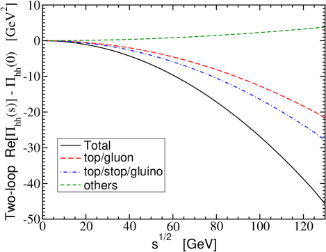
Figure 2: The two-loop contributions to Re$[\Pi_{h^{0}h^{0}}(s)]-\Pi_{h^{0}h^{0}}(0)$ found in section IV, for the model described in the text, as a function of the momentum invariant $s$.

The solid line is the total calculated in section IV of this paper. Various contributions to this are also shown separately: the part coming from diagrams involving a top quark loop and a gluon [the $G_{FF}$ and $G_{\overline{F}\overline{F}}$ terms in eq. (4.1)] are shown as the long-dashed line, the part from other diagrams involving top (s)quarks and gluinos are shown as the dot-dashed line, and all of the remaining contributions are lumped together as the short-dashed line. This shows that, at least for the subset of contributions found in this paper, the deviation from the effective potential approximation comes mostly from top quark loops involving the strong interactions, as one might expect. The relative proportions from different diagrams varies rather strongly with the choice of renormalization scale, but the total has only a small $Q$-dependence. Diagrams involving only squarks contribute less to the quantity Re$[\Pi_{h^{0}h^{0}}(s)]-\Pi_{h^{0}h^{0}}(0)$, because $s\ll m_{\tilde{q}}^{2}$.

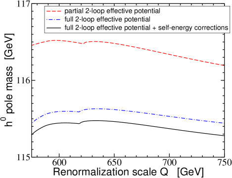
Figure 3: The pole mass of $h^{0}$, computed in various approximations, for the model described in the test, as a function of the renormalization scale $Q$. In each case, the full one-loop self-energy is used in the computation. The dashed line also includes the contributions of the two-loop self-energy in the effective potential approximation, neglecting electroweak couplings. The dot-dashed line includes the contributions of the full two-loop self-energy in the effective potential approximation. The solid line also includes momentum-dependent contributions to the self-energy, as found in section IV.

The resulting pole mass of $h^{0}$ is shown in figure 3, as a function of the choice of renormalization scale $Q$. To make this graph, all of the model parameters including the VEVs are evolved using the two-loop renormalization group equations Martin:1993zk from the defining scale $Q_{0}=640$ GeV to the scale $Q$. The two-loop effective potential is then required to be minimized, determining the values of $\mu$ and $b$ at that scale. Using these parameters as inputs, the dot-dashed line shows the pole mass as calculated in the full effective potential approximation, as in ref. Martin:2002wn . The solid line shows the improved calculation of this paper, using eq. (6.20) for the momentum-dependent self-energy. (For comparison, the dashed line shows the result within a partial two-loop effective potential approximation Zhang:1998bm ; Espinosa:1999zm ; Espinosa:2000df ; Degrassi:2001yf , in which all electroweak effects involving $g,g^{\prime}$ are neglected in the two-loop effective potential.) We see that including the $s$-dependence in the self-energy lowers the prediction for the pole mass, by only about 160 MeV in this model, and nearly independently of the choice of renormalization scale.

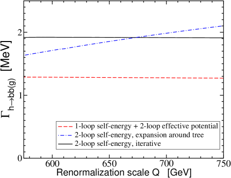
Figure 4: The dependence of the $h^{0}\rightarrow b\overline{b}(g)$ width, obtained from the corresponding contributions to the imaginary part of the pole mass, as a function of the renormalization scale $Q$, in various approximations.

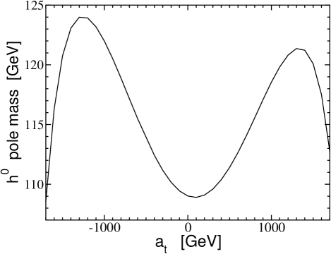
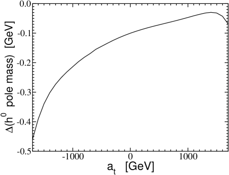
Figure 5: The dependence of the computed $h^{0}$ pole mass on the parameter $a_{t}$, for the model described in the text. The left panel is the same approximation as the solid line of fig. 3. The right panel shows the change in the $h^{0}$ pole mass induced by including the momentum-dependent self-energy, compared to the full two-loop effective potential approximation.

The imaginary part of the pole mass can in principle be used to obtain the physical decay width of $h^{0}$. The contribution from various decay channels can be identified by isolating the imaginary parts due to each one-loop and two-loop contribution to the self-energy. In fig. 4, I show the width corresponding to the decays $h^{0}\rightarrow b\overline{b}$ and $h^{0}\rightarrow b\overline{b}g$. (Not included are spurious imaginary contributions of the self-energy coming from diagrams with Goldstone bosons, which arise because we have not included all of the two-loop self-energy diagrams with non-zero $s$.) The dashed line shows the result coming entirely from the imaginary parts of one-loop bottom-quark diagrams, but using the (real) two-loop effective potential approximation in order to get the kinematics correct by making a reasonable approximation for the real part of the pole mass $s=m^{2}_{h^{0},{\rm pole}}$. The solid line incorporates the additional parts from two-loop diagrams, which therefore includes the effects of gluon emission and one-loop corrections to the $h^{0}b\overline{b}$ vertex and the $b$-quark propagator. The complex pole mass is obtained by iteration of eq. (1.4). In contrast, the dot-dashed line shows the same result, but using the method of expanding the self-energies about the tree-level mass, as in eqs. (1.5)-(1.7). The latter method has a strong $Q$-dependence for the width (although it only makes a difference of at most a few tens of MeV in the real part of the pole mass). This is because the tree-level $h^{0}$ mass is only close to the two-loop mass for renormalization scales near $Q=675$ GeV. Of course, the Higgs decay width is more accurately calculated using other methods (see e.g. Djouadi:1997yw ; Guasch:2003cv and references therein).

I have checked that comparable results obtain for a variety of other MSSM model parameters, including some with large $\tan\beta$. As one illustration, consider the effect of the top squark mixing, which is well-known to have a significant effect on the $h^{0}$ mass. Figure 5 shows the dependence of the computed pole mass on the Lagrangian Higgs-$\tilde{t}_{L}$-$\tilde{t}_{R}$ coupling parameter $a_{t}$, keeping all other parameters (except $\mu$ and $b$) fixed to the values given above. Recall from the definition of ref. Martin:1997ns or effpotMSSM that the off-diagonal entries in the tree-level top-squark squared-mass matrix are $v_{u}a_{t}-\mu y_{t}v_{d}$. Therefore, the top squark mixing angle vanishes for $a_{t}=\mu y_{t}/\tan\beta$ (in this model, about 45 GeV). Figure 5 illustrates that the part of the $h^{0}$ pole mass coming from momentum-dependent effects in the two-loop self-energy is at most a few hundred MeV, and often much less.

In fig. 5, the maximum $h^{0}$ pole mass is obtained for negative $a_{t}$, which at first sight might appear to differ from the results obtained in refs. Espinosa:1999zm ; Espinosa:2000df ; Heinemeyer:1998jw ; Degrassi:2001yf . The reason is that different quantities are being held constant while varying $a_{t}$. In those papers, the on-shell masses are chosen to be held constant, while in this paper the running parameters at the input renormalization scale are held constant instead. The fact that these two slices through parameter space give opposite results for the condition that maximizes the $h^{0}$ pole mass can be immediately seen by comparing eq. (21) with $Q^{2}=m_{\tilde{t}}^{2}$ and eq. (27), both in ref. [22].

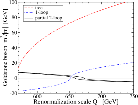
Figure 6: The Goldstone boson mass quantity $m^{2}_{G}/\sqrt{|m^{2}_{G}|}$ in GeV, in the tree-level, one-loop, and partial two-loop approximations, for the model described in the text, as a function of the choice of renormalization scale $Q$. The $G^{0}$ and $G^{\pm}$ lines are not visually distinguishable at tree-level (dashed) and one-loop (dot-dashed) order. The partial two-loop result for $G^{0}$ is the upper solid line and for $G^{\pm}$ is the lower solid line. The full two-loop result for both $G^{0}$ and $G^{\pm}$ should be exactly 0 by construction, since the fields are expanded around the minimum of the Landau gauge two-loop effective potential.

As a numerical study of the effectiveness of the partial two-loop self-energy corrections obtained in this paper, consider the masses of the Goldstone bosons. Because the self-energies are obtained by expanding the Higgs fields around VEVs that minimize the Landau gauge two-loop effective potential, the Goldstone scalars $G^{0}$ and $G^{\pm}$ are exactly massless at two loop order. This means that the matrices

$$m^{2}_{\phi^{0}_{i}}\delta_{ij}+\frac{1}{16\pi^{2}}\Pi^{(1)}_{\phi^{0}_{i}\phi^{0}_{j}}(0)+\frac{1}{(16\pi^{2})^{2}}\Pi^{(2)}_{\phi^{0}_{i}\phi^{0}_{j}}(0),$$ (6.25)

$$m^{2}_{\phi^{\pm}_{i}}\delta_{ij}+\frac{1}{16\pi^{2}}\Pi^{(1)}_{\phi^{+}_{i}\phi^{-}_{j}}(0)+\frac{1}{(16\pi^{2})^{2}}\Pi^{(2)}_{\phi^{+}_{i}\phi^{-}_{j}}(0)$$ (6.26)

each have one 0 eigenvalue. In figure 6, I show the tree-level, one-loop and partial two-loop approximations to the Goldstone boson mass quantity $m^{2}_{G}/\sqrt{|m^{2}_{G}|}$ as a function of the choice of renormalization scale $Q$. Here $m_{G}^{2}$ is defined to be the lowest eigenvalue of respectively the first term, the first two terms, and all three terms with $\Pi^{(2)}$ replaced by $\Pi^{(2)}_{\rm par}$, in eqs. (6.25) and (6.26). Here $\Pi^{(2)}_{\rm par}$ is the partial two-loop approximation from sections IV and V. The effect of the approximation we have made for the two-loop self-energy is seen to be of order only tens of GeV² for the Goldstone boson squared masses at $s=0$, and much smaller than for the one-loop and tree-level approximations.

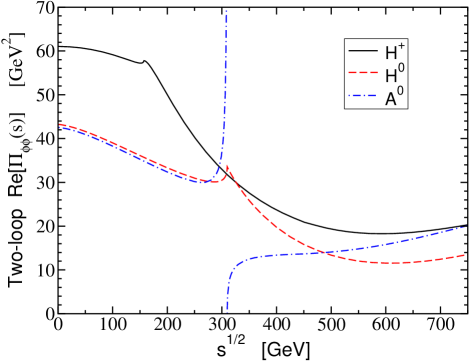
Figure 7: The two-loop contributions to the real parts of the self-energy functions $\Pi_{H^{0}H^{0}}(s)$ and $\Pi_{A^{0}A^{0}}(s)$ (found in section IV) and $\Pi_{H^{+}H^{-}}(s)$ (found in section V), for the model described in the text, as a function of the momentum invariant $s$.

Let us now turn to the effects of the partial two-loop self energy corrections found in this paper on the heavier Higgs scalar bosons $H^{\pm}$, $H^{0}$, and $A^{0}$. These corrections are typically even smaller than for $h^{0}$, both in relative and absolute terms, in part because they have a weaker coupling to virtual top (s)quarks, but also because there are non-trivial cancellations. Figure 7 shows the dependence of the real parts of the diagonal two-loop self-energies for $H^{\pm}$, $H^{0}$, and $A^{0}$, as a function of $s$. Since this model is not far from the decoupling limit, these nearly form an isospin doublet, so the self-energy functions have a similar behavior, especially at larger $s$. Note that the $A^{0}$ self-energy has a singular threshold at $\sqrt{s}=2m_{t}$, due to the effects of massless gluon exchange. The diagrams of the type $V_{FFFFV}$ and $M_{FFFFV}$ in Figure 1 cause threshold behavior proportional to $(1-s/4m_{t}^{2})^{-1/2}$ and ${\rm ln}(1-s/4m_{t}^{2})$, respectively. If the pole mass were in the vicinity of this threshold, these singularities would have to be eliminated by re-summation, a topic beyond the scope of the present paper. In contrast, the threshold behaviors of the $H^{0}$ self-energy at $\sqrt{s}=2m_{t}$ and of the $H^{\pm}$ self-energy at $\sqrt{s}=m_{t}+m_{b}$ are continuous (but not differentiable). In all three cases, I have checked that there is a significant cancellation between the contributions of order $g_{3}^{2}y_{t}^{2}$ and those of order $y_{t}^{4}$. The extent of this cancellation depends on the choice of renormalization scale.

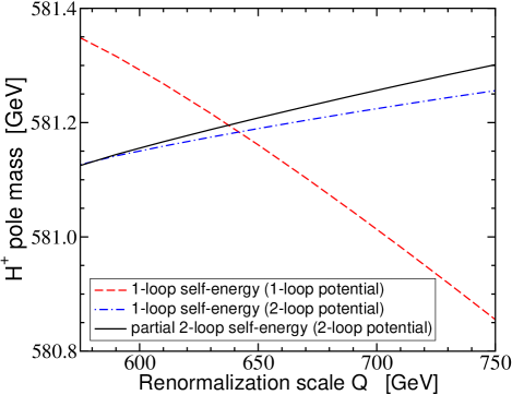
Figure 8: The computed $H^{\pm}$ pole mass for the model described in the text, in various approximations, as a function of the renormalization scale $Q$. The dashed line uses the one-loop effective potential minimization conditions to determine parameters used in the one-loop self-energy. The dot-dashed line uses the two-loop effective potential minimizations condition, and the one-loop self-energy. The solid line uses the two-loop effective potential minimization conditions, and the partial two-loop self-energy as found in section V.

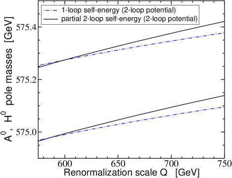
Figure 9: The computed pole masses of $A^{0}$ (lower pair of lines) and $H^{0}$ (upper pair of lines), for the model described in the text, as a function of the renormalization scale $Q$. The approximations are as in figure 8.

The resulting effect of the partial two-loop self-energies on the $H^{\pm}$, $H^{0}$, and $A^{0}$ pole masses is rather small. Figure 8 shows the renormalization scale dependence of the calculated pole mass for the charged Higgs scalars. Here, I do not use the trick of incorporating the effective potential results as was done for $h^{0}$ in eq. (6.20), since the effective potential approximation to the self-energy is not close to valid for the heavier Higgs scalar bosons. Here the dashed line shows the result of a purely one-loop calculation, meaning that the parameters $\mu$, $b$ are fixed from the VEVs by using the one-loop effective potential, and the pole mass is computed using the one-loop self-energy. The dot-dashed line uses the two-loop effective potential to fix $\mu$, $b$, but then uses the one-loop self-energy function to get the pole mass. This is seen to remove much of the renormalization group scale dependence. Using the two-loop self-energy contributions as found in this paper changes the pole mass by only a small amount, (and actually makes the $Q$-dependence slightly worse). The change is much smaller than the dependence on $Q$. The remaining two-loop diagrams involving electroweak gauge couplings and perhaps the three-loop contributions to electroweak symmetry breaking are therefore more important than the diagrams calculated here for this case, and in particular should remove most of the remaining $Q$ dependence in the calculated pole mass. However, the remaining theoretical error is probably already much smaller than future experimental uncertainties Battaglia:2001be ; HiggsLCe .

Very similar results follow for the $A^{0}$ and $H^{0}$ pole masses. They are shown in Figure 9. The same remarks apply here as for $H^{\pm}$.

VII Outlook

In this paper, I have presented partial results for the two-loop self-energy functions of the Higgs scalar bosons in minimal supersymmetry, in the mass-independent and supersymmetric $\overline{\rm DR}^{\prime}$  renormalization scheme. In the case of the lightest Higgs scalar, $h^{0}$, this allows an improved calculation of the gauge-invariant pole mass, which should correspond to the kinematic mass observed at colliders. The size of the corrections was found in typical cases to be of order one to a few hundred MeV. This is significant compared to the eventual experimental uncertainty to be obtained at the LHC and especially at a LC.

To make further progress, it will be necessary to include the remaining two-loop self-energy corrections involving electroweak couplings. This has already been done in the effective potential approximation effpotMSSM ; Martin:2002wn . However, it is precisely for these contributions that the approximation $s=0$ is not always a very good one, particularly for diagrams in which no momentum routing can avoid an electroweak gauge boson. Therefore, it will certainly be necessary to include these contributions in order to reduce the theoretical uncertainties to acceptable levels. It also seems clear that the leading (e.g. $y_{t}^{2}g_{3}^{4}$, $y_{t}^{4}g_{3}^{2}$, and $y_{t}^{6}$) three-loop contributions to the $h^{0}$ pole mass will be necessary, but can be included in the effective potential approximation. These corrections can be estimated in a leading-logarithm approach using the renormalization group, as has recently been done in ref. recentMSSMhiggs . However, we have seen above that the non-logarithmic pieces are not always small compared to the logarithmic ones.

The size of the two-loop effects found above on the heavier Higgs boson masses $H^{\pm}$, $H^{0}$, and $A^{0}$ do not seem to be significant compared to the expected experimental uncertainties. However, I have not conducted an exhaustive search of all of parameter space, and in any case the marginal cost in human effort to include all of the Higgs scalar self-energies at two-loop order is not great, once the two-loop self-energy for $h^{0}$ is included.

Besides calculations in the Higgs sector, it will be necessary to calculate two-loop corrections for the other superpartner masses in order to interpret the results above in realistic situations. This issue is particularly acute in the mass-independent renormalization scheme adopted here, since e.g. the top-quark Yukawa coupling and the top-squark tree-level masses are used as inputs, rather than the physical top-quark and top-squark masses. In order to make meaningful comparisons with higher-order calculations for the Higgs masses done in the on-shell schemes and to future experimental constraints or (hopefully) data, the two-loop mass corrections for the top and bottom quark, the squarks, and the gluino, at least, will be needed. Fortunately, these results are definitely not out of reach.

This work was supported by the National Science Foundation under Grant No. 0140129.

References

(1)
H.E. Haber and G.L. Kane,
Phys. Rept. 117, 75 (1985).
(2)
J.F. Gunion and H.E. Haber,
Nucl. Phys. B 272, 1 (1986)
[Erratum-ibid. B 402, 567 (1993)],
Nucl. Phys. B 278, 449 (1986).
(4)
“ATLAS detector and physics performance. Technical design report. Vol. 2,”
CERN-LHCC-99-15,
and V. Drollinger and A. Sopczak,
Eur. Phys. J. C 3, N1 (2001),
[hep-ph/0102342].
(5)
T. Abe et al. [American Linear Collider Working Group
Collaboration],
“Linear collider physics resource book for Snowmass 2001. 2: Higgs and
supersymmetry studies,”
[hep-ex/0106056].
(6)
J.A. Aguilar-Saavedra et al. [ECFA/DESY LC Physics Working Group
Collaboration],
“TESLA Technical Design Report Part III: Physics at an e+e- Linear
Collider,”
[hep-ph/0106315].
(7)
K. Abe et al. [ACFA Linear Collider Working Group Collaboration],
“Particle physics experiments at JLC,”
[hep-ph/0109166].
(8)
H. E. Haber and R. Hempfling,
Phys. Rev. Lett. 66, 1815 (1991).
(9)
Y. Okada, M. Yamaguchi and T. Yanagida,
Prog. Theor. Phys. 85, 1 (1991),
Phys. Lett. B 262, 54 (1991).
(10)
G. Gamberini, G. Ridolfi and F. Zwirner,
Nucl. Phys. B 331, 331 (1990),
J.R. Ellis, G. Ridolfi and F. Zwirner,
Phys. Lett. B 257, 83 (1991),
Phys. Lett. B 262, 477 (1991).
(11)
R. Barbieri, M. Frigeni and F. Caravaglios,
Phys. Lett. B 258, 167 (1991).
(12)
A. Yamada,
Phys. Lett. B 263, 233 (1991).
(13)
J.R. Espinosa and M. Quiros,
Phys. Lett. B 266, 389 (1991).
(14)
A. Brignole,
Phys. Lett. B 281, 284 (1992).
(15)
M. Drees and M. M. Nojiri,
Phys. Rev. D 45, 2482 (1992),
Nucl. Phys. B 369, 54 (1992).
(16)
P. H. Chankowski, S. Pokorski and J. Rosiek,
Phys. Lett. B 274, 191 (1992).
(17)
J. Kodaira, Y. Yasui and K. Sasaki,
Phys. Rev. D 50, 7035 (1994)
[hep-ph/9311366].
(18)
J.A. Casas, J.R. Espinosa, M. Quiros and A. Riotto,
Nucl. Phys. B 436, 3 (1995)
[Erratum-ibid. B 439, 466 (1995)]
[hep-ph/9407389].
(19)
R. Hempfling and A.H. Hoang,
Phys. Lett. B 331, 99 (1994) [hep-ph/9401219].
H.E. Haber, R. Hempfling and A.H. Hoang,
Z. Phys. C 75, 539 (1997) [hep-ph/9609331].
(20)
D.M. Pierce, J.A. Bagger, K.T. Matchev and R.J. Zhang,
Nucl. Phys. B 491, 3 (1997) [hep-ph/9606211].
(21)
R.J. Zhang,
Phys. Lett. B 447, 89 (1999) [hep-ph/9808299];
(23)
J.R. Espinosa and R.J. Zhang,
Nucl. Phys. B 586, 3 (2000) [hep-ph/0003246].
(24)
S. Heinemeyer, W. Hollik and G. Weiglein,
Phys. Rev. D 58, 091701 (1998) [hep-ph/9803277];
Phys. Lett. B 440, 296 (1998) [hep-ph/9807423];
Comput. Phys. Commun. 124, 76 (2000)
[hep-ph/9812320],
Eur. Phys. J. C 9, 343 (1999) [hep-ph/9812472].
(25)
A. Pilaftsis and C.E. Wagner,
Nucl. Phys. B 553, 3 (1999) [hep-ph/9902371].
M. Carena, J.R. Ellis, A. Pilaftsis and C.E. Wagner,
Nucl. Phys. B 586, 92 (2000) [hep-ph/0003180];
Nucl. Phys. B 625, 345 (2002) [hep-ph/0111245].
(26)
M. Carena
et al,
Nucl. Phys. B 580, 29 (2000) [hep-ph/0001002].
(27)
J.R. Espinosa and I. Navarro,
Nucl. Phys. B 615, 82 (2001) [hep-ph/0104047].
(28)
G. Degrassi, P. Slavich and F. Zwirner,
Nucl. Phys. B 611, 403 (2001) [hep-ph/0105096];
A. Brignole, G. Degrassi, P. Slavich and F. Zwirner,
Nucl. Phys. B 631, 195 (2002) [hep-ph/0112177],
Nucl. Phys. B 643, 79 (2002) [hep-ph/0206101].
(29)
A. Djouadi, J.L. Kneur and G. Moultaka,
[hep-ph/0211331].
(30)
S.P. Martin,
Phys. Rev. D 65, 116003 (2002) [hep-ph/0111209].
(31)
S.P. Martin,
Phys. Rev. D 66, 096001 (2002) [hep-ph/0206136].
(32)
S.P. Martin,
Phys. Rev. D 67, 095012 (2003) [hep-ph/0211366].
(33)
M. Frank, S. Heinemeyer, W. Hollik and G. Weiglein,
[hep-ph/0212037].
(34)
G. Degrassi et al,
Eur. Phys. J. C 28, 133 (2003) [hep-ph/0212020];
(35)
A. Dedes, G. Degrassi and P. Slavich,
Nucl. Phys. B 672, 144 (2003) [hep-ph/0305127];
(36)
J.S. Lee et al,
Comput. Phys. Commun. 156, 283 (2004) [hep-ph/0307377].
(37)
S. Heinemeyer, W. Hollik, F. Merz and S. Penaranda,
[hep-ph/0403228].
(38)
I. Jack et al,
Phys. Rev. D 50, 5481 (1994)
[hep-ph/9407291].
(39)
W. Siegel,
Phys. Lett. B 84, 193 (1979);
D.M. Capper, D.R.T. Jones and P. van Nieuwenhuizen,
Nucl. Phys. B 167, 479 (1980).
(40)
S.P. Martin, “Two-loop scalar self-energies in a general renormalizable
theory at leading order in gauge couplings,” [hep-ph/0312092].
(41)
S.P. Martin,
Phys. Rev. D 68, 075002 (2003) [hep-ph/0307101].
(42) S.P. Martin and D.G. Robertson, in preparation.
(43)
O.V. Tarasov,
Nucl. Phys. B 502, 455 (1997)
[hep-ph/9703319].
(44)
R. Mertig and R. Scharf,
Comput. Phys. Commun. 111, 265 (1998)
hep-ph/9801383.
(45)
M. Caffo, H. Czyz, S. Laporta and E. Remiddi,
Nuovo Cim. A 111, 365 (1998)
[hep-th/9805118];
Acta Phys. Polon. B 29, 2627 (1998)
[hep-th/9807119];
M. Caffo, H. Czyz and E. Remiddi,
Nucl. Phys. B 634, 309 (2002) hep-ph/0203256;
“Numerical evaluation of master integrals from differential equations,”
[hep-ph/0211178], talk given at RADCOR 2002;
M. Caffo, H. Czyz, A. Grzelinska and E. Remiddi,
Nucl. Phys. B 681, 230 (2004)
[hep-ph/0312189].
(46)
G. Weiglein, R. Scharf and M. Bohm,
Nucl. Phys. B 416, 606 (1994) [hep-ph/9310358].
(47)
A. Ghinculov and Y.P. Yao,
Nucl. Phys. B 516, 385 (1998) [hep-ph/9702266];
Phys. Rev. D 63, 054510 (2001)
[hep-ph/0006314].
(48)
S. Willenbrock and G. Valencia,
Phys. Lett. B 259, 373 (1991).
(49)
R.G. Stuart,
Phys. Lett. B 262, 113 (1991),
Phys. Lett. B 272, 353 (1991),
Phys. Rev. Lett. 70, 3193 (1993).
(50)
A. Sirlin,
Phys. Lett. B 267, 240 (1991),
Phys. Rev. Lett. 67, 2127 (1991).
(51)
P. Gambino and P.A. Grassi,
Phys. Rev. D 62, 076002 (2000)
hep-ph/9907254;
P.A. Grassi, B.A. Kniehl and A. Sirlin,
Phys. Rev. Lett. 86, 389 (2001)
hep-th/0005149,
Phys. Rev. D 65, 085001 (2002)
hep-ph/0109228.
(52)
B.A. Kniehl,
Phys. Rev. D 50, 3314 (1994)
[hep-ph/9405299].
(53)
A. Djouadi and P. Gambino,
Phys. Rev. D 51, 218 (1995)
[Erratum-ibid. D 53, 4111 (1996)]
[hep-ph/9406431].
(54)
S.P. Martin and M.T. Vaughn,
Phys. Rev. D 50, 2282 (1994)
[hep-ph/9311340].
(55)
Y. Yamada,
Phys. Rev. D 50, 3537 (1994)
[hep-ph/9401241].
(56)
I. Jack and D.R.T. Jones,
Phys. Lett. B 333, 372 (1994)
[hep-ph/9405233].
(57)
A. Djouadi, J. Kalinowski and M. Spira,
Comput. Phys. Commun. 108, 56 (1998)
[hep-ph/9704448].
(58)
J. Guasch, P. Hafliger and M. Spira,
Phys. Rev. D 68, 115001 (2003)
[hep-ph/0305101].
(59)
M. Battaglia, A. Ferrari, A. Kiiskinen and T. Maki,
“Pair production of charged Higgs bosons at future linear e+ e-
colliders,”
[hep-ex/0112015].