Higgs production at a muon collider in the Two Higgs Doublet Model of type II

Abstract

We calculate Higgs production cross sections at a muon collider in the Two Higgs Doublet Model of type II. The most interesting productions channels are $\mu^{-}\mu^{+}\rightarrow h^{0}Z^{0},H^{0}Z^{0},H^{-}H^{+},A^{0}Z^{0}$ and $H^{\mp}W^{\pm}$. The last channel is compared with the production processes $p\bar{p}\rightarrow H^{\mp}W^{\pm}X$ and $pp\rightarrow H^{\mp}W^{\pm}X$ at the Tevatron and LHC energies, respectively, for large values of $\tan\beta$.

1 Introduction

In this article we calculate neutral and charged Higgs production cross sections at a muon collider in the Two Higgs Doublet Model of type II. The Higgs sector of the Minimal Supersymmetric Standard Model (MSSM) is of this type (tho the model of type II does not require Supersymmetry). Higgs doublets can be added to the Standard Model without upsetting the $Z/W$ mass ratio. Higher dimensional representations upset this ratio [1]. Adding a second complex doublet to the Standard Model results in five Higgs bosons: one pseudoscalar $A^{0}$ (CP-odd scalar), two neutral scalars $H^{0}$ and $h^{0}$ (CP-even scalars), and two charged scalars $H^{+}$ and $H^{-}$. In the Standard Model we only have a single neutral Higgs.

In recent years, some papers have appeared, suggesting the possibility of the construction of a $\mu^{-}\mu^{+}$ collider to detect charged or neutral Higgs bosons [[2], [3]]. The main reason is that in a muon collider, the signal would be much cleaner than in a hadron collider. In this paper, we analyze this possibility studying some production cross sections like: $\mu^{-}\mu^{+}\rightarrow h^{0}Z^{0},H^{0}Z^{0},H^{-}H^{+},A^{0}Z^{0}$ and $H^{\mp}W^{\pm}$ (Sections 2-6).

In Sections 5,6,8,9 we will focus our interest in the production of charged Higgs bosons. There are three ways of producing $H^{\pm}$. One is via $p\bar{p}$ or $pp$ interactions in a hadron collider. In hadron colliders, the signals are overwhelmed by backgrounds due basically to $t\bar{t}$ production [4]. The other ways to produce charged Higgs are $e^{-}e^{+}$ or $\mu^{-}\mu^{+}$ colliders , in which backgrounds are considerably less. In some processes like $\mu^{-}\mu^{+}\rightarrow H^{-}H^{+}$ and $e^{-}e^{+}\rightarrow H^{-}H^{+}$, there is no difference between the cross sections obtained in an $e^{-}e^{+}$ collider or a $\mu^{-}\mu^{+}$ collider. However, in reactions like $\mu^{-}\mu^{+}\rightarrow H^{\mp}W^{\pm}$ and $e^{-}e^{+}\rightarrow H^{\mp}W^{\pm}$, the total cross section is proportional to the square of the mass of the fermion and then $e^{-}e^{+}$ interactions give us very small cross sections. This motivated us to compare in Section 9 the channel $\mu^{-}\mu^{+}\rightarrow H^{\mp}W^{\pm}$ (at $\sqrt{s}=500\textrm{GeV/c}$ and for large values of $\tan\beta$) with the production processes $p\bar{p}\rightarrow H^{\mp}W^{\pm}X$ (at the Tevatron) and $pp\rightarrow H^{\mp}W^{\pm}X$ (at the LHC), to check the feasibility of detecting $H^{\pm}$ using a muon collider.

The influence of radiative corrections in the masses of the Higgs bosons is considered in all the calculations.

2 Higgs bosons masses and radiative corrections

The masses of the neutral Higgs particles, calculated at tree level, are [5]:

$$m_{A^{0}}^{2}=m_{H}^{2}-m_{W}^{2}$$ (1)

$$m_{H^{0}}^{2}=\frac{1}{2}\left[m_{Z}^{2}+m_{A^{0}}^{2}+\left[\left(m_{Z}^{2}-m_{A^{0}}^{2}\right)^{2}+4m_{A^{0}}^{2}m_{Z}^{2}\sin^{2}2\beta\right]^{1/2}\right]$$ (2)

$$m_{h^{0}}^{2}=\frac{1}{2}\left[m_{Z}^{2}+m_{A^{0}}^{2}-\left[\left(m_{Z}^{2}-m_{A^{0}}^{2}\right)^{2}+4m_{A^{0}}^{2}m_{Z}^{2}\sin^{2}2\beta\right]^{1/2}\right]$$ (3)

with $0\leq\beta<\frac{\pi}{2}$

From these relations, the Higgs bosons masses satisfy the bounds:

$$m_{A^{0}}<m_{H}$$ (4)

$$m_{H}>m_{W}$$ (5)

$$m_{h^{0}}\leq m_{Z}$$ (6)

$$m_{Z}\leq m_{H^{0}}\leq\sec\theta_{W}m_{H}$$ (7)

The bound given by (6) practically has been excluded by the present limits on $m_{h^{0}}$ obtained by LEP and CDF [6].

The mixing angle $\alpha$ $(-\pi/2<\alpha\leq 0)$ between the two neutral scalar Higgs fields $H^{0}$, $h^{0}$ is given by

$$\tan\alpha=-\left[\frac{1+F}{1-F}\right]^{1/2}$$ (8)

$$F=\frac{\left(1-\tan^{2}\beta\right)}{\left(1+\tan^{2}\beta\right)G}\left[1-\frac{m_{Z}^{2}}{m_{H}^{2}}-\frac{m_{W}^{2}}{m_{H}^{2}}\right]$$ (9)

$$G=\left[\left(1-\frac{m_{W}^{2}}{m_{H}^{2}}+\frac{m_{Z}^{2}}{m_{H}^{2}}\right)^{2}-4\left(\frac{m_{Z}^{2}}{m_{H}^{2}}\right)\left(1-\frac{m_{W}^{2}}{m_{H}^{2}}\right)\left(\frac{1-\tan^{2}\beta}{1+\tan^{2}\beta}\right)^{2}\right]^{1/2}$$ (10)

In terms of $m_{H}$ and $G$ Equations (2) and (3) are:

$$m_{H^{0}}^{2}=\frac{1}{2}m_{H}^{2}\left[1-\frac{m_{W}^{2}}{m_{H}^{2}}+\frac{m_{Z}^{2}}{m_{H}^{2}}+G\right]$$ (11)

$$m_{h^{0}}^{2}=\frac{1}{2}m_{H}^{2}\left[1-\frac{m_{W}^{2}}{m_{H}^{2}}+\frac{m_{Z}^{2}}{m_{H}^{2}}-G\right]$$ (12)

Taking into account radiative corrections, (2) and (3) can be written as [see [7], [8]]:

$$m_{H^{0}}^{2}=\frac{1}{2}\{m_{A}^{2}+m_{Z}^{2}+\Delta_{t}+\Delta_{b}$$ (13)

$$+\left[\left(\left(m_{A}^{2}-m_{Z}^{2}\right)\cos 2\beta+\Delta_{t}-\Delta_{b}\right)^{2}+\left(m_{A}^{2}+m_{Z}^{2}\right)^{2}\sin^{2}2\beta\right]^{1/2}\}$$

$$m_{h^{0}}^{2}=\frac{1}{2}\{m_{A}^{2}+m_{Z}^{2}+\Delta_{t}+\Delta_{b}$$ (14)

$$-\left[\left(\left(m_{A}^{2}-m_{Z}^{2}\right)\cos 2\beta+\Delta_{t}-\Delta_{b}\right)^{2}+\left(m_{A}^{2}+m_{Z}^{2}\right)^{2}\sin^{2}2\beta\right]^{1/2}\}$$

where:

$$\Delta_{b}=\frac{3\sqrt{2}m_{b}^{4}G_{F}\left(1+\tan^{2}\beta\right)}{2\pi^{2}}ln\left(\frac{M_{sb}^{2}}{m_{b}^{2}}\right)$$ (15)

and

$$\Delta_{t}=\frac{3\sqrt{2}m_{t}^{4}G_{F}\left(1+\tan^{2}\beta\right)}{2\pi^{2}\tan^{2}\beta}ln\left(\frac{M_{st}^{2}}{m_{t}^{2}}\right)$$ (16)

$M_{sb}$ and $M_{st}$ are the masses of the sbottom and stop (the scalar superpartners of the bottom and top quarks).

Equation (1) is practically unaffected by radiative corrections. According to (14) $m_{h^{0}}$ increases as the value of $m_{A}$ increases. Then, for very large values of $m_{A}$ we can set an upper bound for $m_{h^{0}}$:

$$m_{h^{0}}\leq m_{h^{0}}(m_{A^{0}}\rightarrow\infty)=m_{Z}^{2}\left(\frac{1-\tan^{2}\beta}{1+\tan^{2}\beta}\right)^{2}+\frac{\Delta_{t}\tan^{2}\beta}{\left(1+\tan^{2}\beta\right)}+\frac{\Delta_{b}}{\left(1+\tan^{2}\beta\right)}$$ (17)

Taking $m_{b}=4.3$ $\textrm{GeV/c}^{2}$, $m_{t}=174.3\textrm{GeV/c}^{2}$, $M_{st}\sim M_{sb}\sim 1\textrm{TeV}$ [7] and $m_{Z}=91.1876\textrm{GeV/c}^{2}$ we obtain:

$$\Delta_{b}=1.123\times 10^{-6}\left(1+\tan^{2}\beta\right)m_{Z}^{2}$$ (18)

$$\Delta_{t}=0.9723m_{Z}^{2}\frac{\left(1+\tan^{2}\beta\right)}{\tan^{2}\beta}$$ (19)

The contribution of the b-quark loop is negligible. Using Equations (18) and (19), (17) can be expressed as:

$$m_{h^{0}}\leq m_{Z}\left[\left(\frac{1-\tan^{2}\beta}{1+\tan^{2}\beta}\right)^{2}+0.9723\right]^{1/2}$$ (20)

For large values of $\tan\beta$ ($\tan\beta\rightarrow\infty$) we obtain the limit

$$m_{h^{0}}\leq 1.4044m_{Z}=128.062\textrm{GeV/c}^{2}$$ (21)

The upper bound on $m_{h^{0}}$ is raised by radiative corrections from $m_{Z}$ to 128.062 $\textrm{GeV/c}^{2}$ for stop masses of order 1 TeV.

Considering radiative corrections, we can write, for the masses of the neutral Higgs scalars:

$$m_{H^{0}}^{2}=\frac{1}{2}m_{H}^{2}\left[1-\frac{m_{W}^{2}}{m_{H}^{2}}+\frac{m_{Z}^{2}}{m_{H}^{2}}+\frac{\Delta_{t}}{m_{H}^{2}}+G_{rc}\right]$$ (22)

$$m_{h^{0}}^{2}=\frac{1}{2}m_{H}^{2}\left[1-\frac{m_{W}^{2}}{m_{H}^{2}}+\frac{m_{Z}^{2}}{m_{H}^{2}}+\frac{\Delta_{t}}{m_{H}^{2}}-G_{rc}\right]$$ (23)

$$G_{rc}=[\left(1-\frac{m_{W}^{2}}{m_{H}^{2}}+\frac{m_{Z}^{2}}{m_{H}^{2}}\right)^{2}-4\left(\frac{m_{Z}^{2}}{m_{H}^{2}}\right)\left(1-\frac{m_{W}^{2}}{m_{H}^{2}}\right)\left(\frac{1-\tan^{2}\beta}{1+\tan^{2}\beta}\right)^{2}$$ (24)

$$+2\left(\frac{\Delta_{t}}{m_{H}^{2}}\right)\left(1-\frac{m_{W}^{2}}{m_{H}^{2}}-\frac{m_{Z}^{2}}{m_{H}^{2}}\right)\left(\frac{1-\tan^{2}\beta}{1+\tan^{2}\beta}\right)+\left(\frac{\Delta_{t}}{m_{H}^{2}}\right)^{2}]^{1/2}$$

With radiative corrections, the value of the $\alpha$ parameter is:

$$\tan\alpha=-\left[\frac{1+F_{rc}}{1-F_{rc}}\right]^{1/2}$$ (25)

$$F_{rc}=\frac{\left[\left(\frac{1-\tan^{2}\beta}{1+\tan^{2}\beta}\right)\left(1-\frac{m_{Z}^{2}}{m_{H}^{2}}-\frac{m_{W}^{2}}{m_{H}^{2}}\right)+\frac{\Delta_{t}}{m_{H}^{2}}\right]}{G_{rc}}$$ (26)

Additionally we have:

$$\sin 2\alpha=-\frac{2\tan\beta}{\left(1+\tan^{2}\beta\right)}\frac{\left(1-\frac{m_{W}^{2}}{m_{H}^{2}}+\frac{m_{Z}^{2}}{m_{H}^{2}}\right)}{G_{rc}}$$ (27)

3 Production of $h^{0}$ , $H^{0}$

From the Feynman diagrams in Figure 1 and the corresponding Feynman rules given in reference [9], we obtain the differential cross section for the reaction $\mu^{-}\mu^{+}\rightarrow h^{0}Z^{0}$ in the center of mass system

$$\frac{d\sigma}{d\Omega}(\mu^{-}\mu^{+}\rightarrow h^{0}Z^{0})=\frac{1}{64\pi^{2}s^{2}}G_{F}^{2}m_{Z}^{4}\left|C_{Z}\right|^{2}\Lambda^{1/2}(s,m_{h^{0}}^{2},m_{Z}^{2})$$ (28)

$$\left[\left(g_{A}^{\mu}\right)^{2}+\left(g_{V}^{\mu}\right)^{2}\right]\left[8sm_{Z}^{2}+\Lambda(s,m_{h^{0}}^{2},m_{Z}^{2})sin^{2}\theta\right]$$

where

$$g_{A}^{\mu}=-\frac{1}{2}$$ (29)

$$g_{V}^{\mu}=-\frac{1}{2}+2\sin^{2}\theta_{W}$$

$$\Lambda(a,b,c)=a^{2}+b^{2}+c^{2}-2ab-2ac-2bc$$ (30)

$$C_{Z}=\frac{\sin\left(\beta-\alpha\right)}{\left(s-m_{Z}^{2}+im_{Z}\Gamma_{Z}\right)}$$ (31)

$\Gamma_{Z}$ is the total decay width of the $Z^{0}$ and $\theta$ is the scattering angle in the center of mass system.

Figure 1: Feynman diagrams corresponding to the production of $h^{0}$ or $H^{0}$ in the channel $\mu^{-}\mu^{+}\rightarrow h^{0}Z^{0}$.

The total cross section corresponding to $\mu^{-}\mu^{+}\rightarrow h^{0}Z^{0}$ is obtained integrating Equation (28):

$$\sigma(\mu^{-}\mu^{+}\rightarrow h^{0}Z^{0})=\frac{G_{F}^{2}m_{Z}^{4}\left(\tan\beta-\tan\alpha\right)^{2}}{48\pi s^{2}\left(1+\tan^{2}\alpha\right)\left(1+\tan^{2}\beta\right)}$$ (32)

$$\times\frac{\left(1-4\sin^{2}\theta_{W}+8\sin^{4}\theta_{W}\right)}{\left[\left(s-m_{Z}^{2}\right)^{2}+m_{Z}^{2}\Gamma_{Z}^{2}\right]}\left[12sm_{Z}^{2}+\Lambda(s,m_{h^{0}}^{2},m_{Z}^{2})\right]$$

$$\times\Lambda^{1/2}(s,m_{h^{0}}^{2},m_{Z}^{2})\times\left(3.8938\times 10^{11}\right)\textrm{fb}$$

In Figures 2 and 3 , the total cross section for $\mu^{-}\mu^{+}\rightarrow h^{0}Z^{0}$, is plotted as a function $m_{h^{0}}$ for several values of $\sqrt{s}$ and $\tan\beta$. These total cross sections were plotted considering the radiative corrections of the masses given by Equations (23), (24), (25) and (26). According to these graphs, the total cross section becomes important in the mass interval $118\leq m_{h^{0}}\leq 128[\textrm{GeV/c}^{2}]$.

Figure 2: Total cross section for the process $\mu^{-}\mu^{+}\rightarrow h^{0}Z^{0}$ as a function of $m_{h^{0}}$. We have taken $\sqrt{s}=500\textrm{GeV/c}$ and $\tan\beta=30$.

Figure 3: Total cross section for the process $\mu^{-}\mu^{+}\rightarrow h^{0}Z^{0}$ as a function of $m_{h^{0}}$. We have taken $\sqrt{s}=400\textrm{GeV/c}$ and $\tan\beta=50$.

The Standard Model cross section is:

$$\sigma(\mu^{-}\mu^{+}\rightarrow h_{SM}^{0}Z^{0})_{SM}=\frac{G_{F}^{2}m_{Z}^{4}}{48\pi s^{2}}\frac{\left(1-4\sin^{2}\theta_{W}+8\sin^{4}\theta_{W}\right)}{\left[\left(s-m_{Z}^{2}\right)^{2}+m_{Z}^{2}\Gamma_{Z}^{2}\right]}$$

$$\times\left[12sm_{Z}^{2}+\Lambda(s,m_{h_{SM}^{0}}^{2},m_{Z}^{2})\right]$$

$$\times\Lambda^{1/2}(s,m_{h_{SM}^{0}}^{2},m_{Z}^{2})\times\left(3.8938\times 10^{11}\right)\textrm{fb}$$ (33)

where $h_{SM}$ is the Standard Model higgs boson.

The production cross section corresponding to $e^{-}e^{+}\rightarrow h^{0}Z^{0}$ is given by an expression identical to (32). In terms of the cross section $\sigma\left(e^{-}e^{+}\rightarrow\mu^{-}\mu^{+}\right)$ we can write:

$$\frac{\sigma\left(e^{-}e^{+}\rightarrow h^{0}Z^{0}\right)}{\sigma\left(e^{-}e^{+}\rightarrow\mu^{-}\mu^{+}\right)}=\frac{1}{128s}\frac{\left(\tan\beta-\tan\alpha\right)^{2}}{\left(1+\tan^{2}\alpha\right)\left(1+\tan^{2}\beta\right)}\Lambda^{1/2}(s,m_{h^{0}}^{2},m_{Z}^{2})$$ (34)

$$\times\frac{\left(1-4\sin^{2}\theta_{W}+8\sin^{4}\theta_{W}\right)}{\sin^{4}\theta_{W}\left(1-\sin^{2}\theta_{W}\right)^{2}}\frac{\left[12sm_{Z}^{2}+\Lambda(s,m_{h^{0}}^{2},m_{Z}^{2})\right]}{\left[\left(s-m_{Z}^{2}\right)^{2}+m_{Z}^{2}\Gamma_{Z}^{2}\right]}$$

Equation (34) is plotted in Figure 4, as a function of $m_{h^{0}}$ for $\sqrt{s}=500\textrm{GeV/c}$ and $\tan\beta=30$.

Figure 4: Total cross section $\sigma(e^{-}e^{+}\rightarrow h^{0}Z^{0})$ compared with the cross section $\sigma(e^{-}e^{+}\rightarrow\mu^{-}\mu^{+})$ as a function of $m_{h^{0}}$. We have taken $\sqrt{s}=500\textrm{GeV/c}$ and $\tan\beta=30$.

The total cross section corresponding to $\mu^{-}\mu^{+}\rightarrow H^{0}Z^{0}$ is obtained from Equation (32) replacing $\left(\tan\beta-\tan\alpha\right)^{2}$ by $\left(1+\tan\beta\tan\alpha\right)^{2}$ in the numerator and $m_{h^{0}}$ by $m_{H^{0}}$. This production cross section is plotted in Figures 5, 6 as a function of $m_{H^{0}}$ for $\sqrt{s}=500\textrm{GeV/c}$ and $\tan\beta=30$, without and with mass radiative corrections, respectively. In Figure 7 we show the ratio between the production cross section $\sigma\left(e^{-}e^{+}\rightarrow H^{0}Z^{0}\right)$ and the cross section $\sigma\left(e^{-}e^{+}\rightarrow\mu^{-}\mu^{+}\right)$ in terms of $m_{H^{0}}$. The radiatively corrected masses total cross section is shown in Figure 8. Figures 6 and 8 show the importance of the radiative corrections of the masses in the processes $\mu^{-}\mu^{+}\rightarrow H^{0}Z^{0}$ and $e^{-}e^{+}\rightarrow H^{0}Z^{0}$.

Figure 5: Total cross section for the process $\mu^{-}\mu^{+}\rightarrow H^{0}Z^{0}$ as a function of $m_{H^{0}}$. The radiative corrections of the masses were not taken into account. We have taken $\sqrt{s}=500\textrm{GeV/c}$ and $\tan\beta=30$.

Figure 6: Radiatively corrected masses total cross section for the process $\mu^{-}\mu^{+}\rightarrow H^{0}Z^{0}$ as a function of $m_{H^{0}}$. We have taken $\sqrt{s}=500\textrm{GeV/c}$ and $\tan\beta=30$.

Figure 7: Total cross section for the process $e^{-}e^{+}\rightarrow H^{0}Z^{0}$ compared with the cross section $\sigma(e^{-}e^{+}\rightarrow\mu^{-}\mu^{+})$ as a function of $m_{H^{0}}$. We have taken $\sqrt{s}=\textrm{500 GeV/c}$ and $\tan\beta=30$. The radiative corrections of the masses were not taken into account.

Figure 8: Radiatively corrected masses total cross section for the process $e^{-}e^{+}\rightarrow H^{0}Z^{0}$ compared with the cross section $\sigma(e^{-}e^{+}\rightarrow\mu^{-}\mu^{+})$ as a function of $m_{H^{0}}$. We have taken $\sqrt{s}=500\textrm{GeV/c}$ and $\tan\beta=30$.

4 Production of $A^{0}$

From the Feynman diagrams of Figure 9 and the Feynman rules given in [9], we obtain the differential cross section for the production process $\mu^{-}\mu^{+}\rightarrow A^{0}Z^{0}$ in the center of mass system:

Figure 9: Feynman diagrams corresponding to the production of $A^{0}$ in the channel $\mu^{-}\mu^{+}\rightarrow A^{0}Z^{0}$.

$$\frac{d\sigma}{d\Omega}(\mu^{-}\mu^{+}\rightarrow A^{0}Z^{0})=\frac{1}{64\pi^{2}s}\Lambda^{1/2}\left(s,m_{A^{0}}^{2},m_{Z}^{2}\right)G_{F}^{2}m_{\mu}^{2}$$ (35)

$$\{C_{Hb}^{2}\Lambda\left(s,m_{A^{0}}^{2},m_{Z}^{2}\right)+\left[\left(g_{A}^{\mu}\right)^{2}+\left(g_{V}^{\mu}\right)^{2}\right]$$

$$[\tan^{2}\beta\left(1+\frac{\Lambda\left(s,m_{A^{0}}^{2},m_{Z}^{2}\right)m_{Z}^{2}\sin^{2}\theta}{2st^{2}}\right)$$

$$+\tan^{2}\beta\left(1+\frac{\Lambda\left(s,m_{A^{0}}^{2},m_{Z}^{2}\right)m_{Z}^{2}\sin^{2}\theta}{2su^{2}}\right)]$$

$$+2g_{A}^{\mu}\tan\beta C_{Hb}\left[\frac{m_{A^{0}}^{2}m_{Z}^{2}}{t}-\frac{\Lambda\left(s,m_{A^{0}}^{2},m_{Z}^{2}\right)\sin^{2}\theta}{4t}-t\right]$$

$$+2g_{A}^{\mu}\tan\beta C_{Hb}\left[\frac{m_{A^{0}}^{2}m_{Z}^{2}}{u}-\frac{\Lambda\left(s,m_{A^{0}}^{2},m_{Z}^{2}\right)\sin^{2}\theta}{4u}-u\right]$$

$$+2\tan^{2}\beta\left[\left(g_{V}^{\mu}\right)^{2}-\left(g_{A}^{\mu}\right)^{2}\right][\frac{m_{A^{0}}^{2}m_{Z}^{2}}{ut}-\frac{\Lambda\left(s,m_{A^{0}}^{2},m_{Z}^{2}\right)\sin^{2}\theta}{4ut}$$

$$+\frac{\Lambda\left(s,m_{A^{0}}^{2},m_{Z}^{2}\right)m_{Z}^{2}\sin^{2}\theta}{2sut}]\}$$

where $g_{A}^{\mu}$ and $g_{V}^{\mu}$ are given by (29); $s$,$t$,$u$ are the Mandelstam invariant variables and

$$C_{Hb}=\frac{\left(\frac{1}{2}\sin 2\alpha+\tan\beta\sin^{2}\alpha\right)}{\left(s-m_{h^{0}}^{2}\right)}-\frac{\left(\frac{1}{2}\sin 2\alpha-\tan\beta\cos^{2}\alpha\right)}{\left(s-m_{H^{0}}^{2}\right)}$$ (36)

To obtain the total cross section, we integrate Equation (35) over the solid angle $\Omega$.

$$\sigma(\mu^{-}\mu^{+}\rightarrow A^{0}Z^{0})=\frac{G_{F}^{2}m_{\mu}^{2}}{16\pi s^{2}}\{\Lambda^{1/2}\left(s,m_{A^{0}}^{2},m_{Z}^{2}\right)[sC_{Hb}^{2}\Lambda\left(s,m_{A^{0}}^{2},m_{Z}^{2}\right)$$ (37)

$$+4\tan^{2}\beta\sin^{2}\theta_{W}\left(1-2\sin^{2}\theta_{W}\right)\left(s-2m_{Z}^{2}\right)+2s\tan\beta C_{Hb}$$

$$\times\left(m_{A^{0}}^{2}+m_{Z}^{2}-s\right)+\left(1-4\sin^{2}\theta_{W}+8\sin^{4}\theta_{W}\right)$$

$$\times\tan^{2}\beta\left(s-4m_{Z}^{2}\right)]+4m_{Z}^{2}\tan\beta f\left(s,m_{A^{0}}^{2},m_{Z}^{2}\right)$$

$$\times[-sC_{Hb}m_{A^{0}}^{2}+\frac{1}{2}\tan\beta\left(1-4\sin^{2}\theta_{W}+8\sin^{4}\theta_{W}\right)\left(m_{A^{0}}^{2}+m_{Z}^{2}-s\right)$$

$$-4\frac{\sin^{2}\theta_{W}\left(1-2\sin^{2}\theta_{W}\right)\tan\beta m_{A^{0}}^{2}\left(s-m_{Z}^{2}\right)}{\left(m_{A^{0}}^{2}+m_{Z}^{2}-s\right)}]\}$$

$$\times\left(3.8938\times 10^{11}\right)\textrm{fb}$$

where

$$f\left(s,m_{A^{0}}^{2},m_{Z}^{2}\right)\equiv\ln\left|\frac{m_{A^{0}}^{2}+m_{Z}^{2}-s+\Lambda^{1/2}\left(s,m_{A^{0}}^{2},m_{Z}^{2}\right)}{m_{A^{0}}^{2}+m_{Z}^{2}-s-\Lambda^{1/2}\left(s,m_{A^{0}}^{2},m_{Z}^{2}\right)}\right|$$ (38)

Note that if $m_{A^{0}}=\sqrt{s}-m_{Z}$, then we have, $\Lambda\left(s,m_{A^{0}}^{2},m_{Z}^{2}\right)=0$ and $f\left(s,m_{A^{0}}^{2},m_{Z}^{2}\right)$ = 0. Therefore $\sigma(\mu^{-}\mu^{+}\rightarrow A^{0}Z^{0})=0$.

Figure 10 shows the total cross section $\sigma(\mu^{-}\mu^{+}\rightarrow A^{0}Z^{0})$ as a function of $m_{A^{0}}$ for $\sqrt{s}=500\textrm{GeV/c}$ and $\tan\beta=30,50$. The total cross section is not affected by radiative corrections of the masses. From Figure 10 we can see that cross sections are important for large values of $\tan\beta$.

The total cross section corresponding to $e^{-}e^{+}\rightarrow A^{0}Z^{0}$ can be obtained from Equation (37) replacing $m_{\mu}$ by $m_{e}$:

$$\frac{\sigma(e^{-}e^{+}\rightarrow A^{0}Z^{0})}{\sigma(\mu^{-}\mu^{+}\rightarrow A^{0}Z^{0})}=\left(\frac{m_{e}}{m_{\mu}}\right)^{2}=2.34\cdot 10^{-5}.$$ (39)

Figure 10: Total cross section for the process $\mu^{-}\mu^{+}\rightarrow A^{0}Z^{0}$ as a function of $m_{A^{0}}$. We have taken $\sqrt{s}=500\textrm{GeV/c}$ and $\tan\beta=30,50$. The total cross section is not affected by radiative corrections of the masses.

5 Production of $H^{\pm}$

From the Feynman diagrams of Figure 11 we obtain the differential cross section in the center of mass system for the process $\mu^{-}\mu^{+}\rightarrow H^{-}W^{+}$:

$$\frac{d\sigma}{d\Omega}(\mu^{-}\mu^{+}\rightarrow H^{-}W^{+})=\frac{1}{64\pi^{2}s}\Lambda^{1/2}\left(s,m_{H}^{2},m_{W}^{2}\right)G_{F}^{2}m_{\mu}^{2}$$ (40)

$$\times\{\left[C_{Hb}^{2}+C_{Ab}^{2}\right]\Lambda\left(s,m_{H}^{2},m_{W}^{2}\right)+2\left(\frac{\tan\beta}{t}\right)^{2}$$

$$\times\left[\frac{\Lambda\left(s,m_{H}^{2},m_{W}^{2}\right)\sin^{2}\theta m_{W}^{2}}{2s}+t^{2}\right]-2\left(\frac{\tan\beta}{t}\right)\left(C_{Ab}+C_{Hb}\right)$$

$$\times\left[-t^{2}-\frac{1}{4}\Lambda\left(s,m_{H}^{2},m_{W}^{2}\right)\sin^{2}\theta+m_{W}^{2}m_{H}^{2}\right]\}$$

Figure 11: Feynman diagrams corresponding to the production of $H^{-}$ in the channel $\mu^{-}\mu^{+}\rightarrow H^{-}W^{+}$.

where $C_{Hb}$ is given by Equation (36) and

$$C_{Ab}=\frac{\tan\beta}{\left(s-m_{A^{0}}^{2}\right)}$$ (41)

The differential cross section corresponding to $\mu^{-}\mu^{+}\rightarrow H^{+}W^{-}$ is obtained from (40) by replacing $t$ by $u$.

The integration of (40) over the solid angle $\Omega$ give us the total cross section:

$$\sigma(\mu^{-}\mu^{+}\rightarrow H^{-}W^{+})=\frac{G_{F}^{2}m_{\mu}^{2}}{16\pi s^{2}}\{s\Lambda^{3/2}\left(s,m_{H}^{2},m_{W}^{2}\right)\left[C_{Hb}^{2}+C_{Ab}^{2}\right]$$ (42)

$$+2\tan\beta\Lambda^{1/2}\left(s,m_{H}^{2},m_{W}^{2}\right)[\tan\beta\left(s-4m_{W}^{2}\right)$$

$$+\left(C_{Ab}+C_{Hb}\right)s\left(m_{H}^{2}+m_{W}^{2}-s\right)]+4m_{W}^{2}\tan\beta f\left(s,m_{H}^{2},m_{W}^{2}\right)$$

$$\left[\tan\beta\left(m_{H}^{2}+m_{W}^{2}-s\right)-\left(C_{Ab}+C_{Hb}\right)sm_{H}^{2}\right]\}$$

$$\times\left(3.8938\times 10^{11}\right)\textrm{fb}$$

where

$$f\left(s,m_{H}^{2},m_{W}^{2}\right)=\ln\left|\frac{m_{H}^{2}+m_{W}^{2}-s+\Lambda^{1/2}\left(s,m_{H}^{2},m_{W}^{2}\right)}{m_{H}^{2}+m_{W}^{2}-s-\Lambda^{1/2}\left(s,m_{H}^{2},m_{W}^{2}\right)}\right|$$ (43)

For the process $\mu^{-}\mu^{+}\rightarrow H^{+}W^{-}$ we obtain:

$$\sigma(\mu^{-}\mu^{+}\rightarrow H^{+}W^{-})=\sigma(\mu^{-}\mu^{+}\rightarrow H^{-}W^{+})$$ (44)

and then

$$\sigma(\mu^{-}\mu^{+}\rightarrow H^{\pm}W^{\mp})=2\sigma(\mu^{-}\mu^{+}\rightarrow H^{-}W^{+})$$ (45)

Observe that $\sigma(\mu^{-}\mu^{+}\rightarrow H^{\pm}W^{\mp})=0$ if $m_{H}=\sqrt{s}-m_{W}$.

The total cross section corresponding to $\mu^{-}\mu^{+}\rightarrow H^{\mp}W^{\pm}$ is given in Figure 12 for $\sqrt{s}=500\textrm{GeV/c}$ and $\tan\beta=20,30,50$. This total cross section is not affected by radiative corrections of the masses. From Figure 12 we see that $\sigma(\mu^{-}\mu^{+}\rightarrow H^{\mp}W^{\pm})\gtrsim 5\textrm{fb}$ for $\tan\beta\geq 20$ in the mass interval $100\leq m_{H}\leq 400[\textrm{GeV/c}^{2}]$.

For the process $e^{-}e^{+}\rightarrow H^{\mp}W^{\pm}$, the total cross section is obtained from Equations (42), (45) replacing $m_{\mu}$ by $m_{e}$. This cross section is smaller than the one ploted in Figure 12 by a factor $m_{e}^{2}/m_{\mu}^{2}=2.34\cdot 10^{-5}$.

Figure 12: Total cross section for the process $\mu^{-}\mu^{+}\rightarrow H^{\mp}W^{\pm}$ as a function of $m_{H}$. We have taken $\sqrt{s}=500\textrm{GeV/c}$ and $\tan\beta=20,30,50$. The radiative corrections of the masses are negligible.

6 Production of charged Higgs boson pairs

From the Feynman diagrams of Figure 13, the differential cross section in the center of mass system corresponding to $\mu^{-}\mu^{+}\rightarrow H^{-}H^{+}$ is

Figure 13: Feynman diagrams corresponding to the production of charged higgs boson pairs in the channel $\mu^{-}\mu^{+}\rightarrow H^{-}H^{+}$.

$$\frac{d\sigma}{d\Omega}(\mu^{-}\mu^{+}\rightarrow H^{-}H^{+})=\frac{G_{F}^{2}m_{W}^{4}}{8\pi^{2}s}\left(1-4\frac{m_{H}^{2}}{s}\right)^{1/2}\{s\left(s-4m_{H}^{2}\right)\sin^{2}\theta$$ (46)

$$\left[\frac{1}{8}\left|C_{1}\right|^{2}\left[\left(g_{A}^{\mu}\right)^{2}+\left(g_{V}^{\mu}\right)^{2}\right]+2\left(\frac{\sin^{2}\theta_{W}}{s}\right)^{2}-\left(\frac{\sin^{2}\theta_{W}}{s}\right)\Re{(C_{1})}g_{V}^{\mu}\right]$$

$$+2m_{\mu}^{2}[\left(s-4m_{H}^{2}\right)[\frac{\left|C_{1}\right|^{2}}{4}\left(\cos^{2}\theta\left(g_{V}^{\mu}\right)^{2}-\sin^{2}\theta\left(g_{A}^{\mu}\right)^{2}\right)$$

$$+4\left(\frac{\sin^{2}\theta_{W}}{s}\right)^{2}\cos^{2}\theta-2\left(\frac{\sin^{2}\theta_{W}}{s}\right)\Re{(C_{1})}g_{V}^{\mu}\cos^{2}\theta]$$

$$+\frac{1}{4}\left(C^{Hh}\right)^{2}s+\left(s\left(s-4m_{H}^{2}\right)\right)^{1/2}$$

$$\times\cos\theta C^{Hh}\left(\frac{1}{2}g_{V}^{\mu}\Re{(C_{1})}-2\left(\frac{\sin^{2}\theta_{W}}{s}\right)\right)]\}$$

where $g_{A}^{\mu}$ and $g_{V}^{\mu}$ are given by Equation (29),

$$C_{1}\equiv\frac{\cos(2\theta_{W})}{\cos^{2}\theta_{W}}\frac{1}{\left(s-m_{Z}^{2}+im_{Z}\Gamma_{Z}\right)},$$ (47)

$$C^{Hh}=\frac{a_{1}}{\left(s-m_{H^{0}}^{2}\right)}-\frac{a_{2}}{\left(s-m_{h^{0}}^{2}\right)},$$ (48)

$$a_{1}=[\cos^{2}\alpha+\frac{\tan\beta\sin 2\alpha}{2}-\frac{m_{Z}}{2m_{W}\cos\theta_{W}}$$ (49)

$$\frac{\left(1-\tan^{2}\beta\right)}{\left(1+\tan^{2}\beta\right)}\left(\cos^{2}\alpha-\frac{\tan\beta\sin 2\alpha}{2}\right)],$$

$$a_{2}=[\frac{\tan\beta\sin 2\alpha}{2}-\sin^{2}\alpha+\frac{m_{Z}}{2m_{W}\cos\theta_{W}}$$ (50)

$$\frac{\left(1-\tan^{2}\beta\right)}{\left(1+\tan^{2}\beta\right)}\left(\sin^{2}\alpha+\frac{\tan\beta\sin 2\alpha}{2}\right)]$$

The integration of (46) give us the total cross section for the process $\mu^{-}\mu^{+}\rightarrow H^{-}H^{+}$:

$$\sigma\left(\mu^{+}\mu^{-}\rightarrow H^{+}H^{-}\right)=\sigma\left(\mu^{-}\mu^{+}\rightarrow H^{-}H^{+}\right)=\frac{2m_{W}^{4}G_{F}^{2}\sin^{4}\theta_{W}}{3\pi s}$$ (51)

$$\left(1-\frac{4m_{H}^{2}}{s}\right)^{3/2}\{[1+\frac{\left(1-2\sin^{2}\theta_{W}\right)^{2}\left(1+\left(4\sin^{2}\theta_{W}-1\right)^{2}\right)}{64\sin^{4}\theta_{W}\cos^{4}\theta_{W}}$$

$$\times\frac{1}{\left[\left(1-\frac{m_{Z}^{2}}{s}\right)^{2}+\left(\frac{M_{Z}\Gamma_{Z}}{s}\right)^{2}\right]}-\frac{\left(1-2\sin^{2}\theta_{W}\right)\left(4\sin^{2}\theta_{W}-1\right)}{4\sin^{2}\theta_{W}\cos^{2}\theta_{W}}$$

$$\times\frac{\left(1-\frac{m_{Z}^{2}}{s}\right)}{\left[\left(1-\frac{m_{Z}^{2}}{s}\right)^{2}+\left(\frac{M_{Z}\Gamma_{Z}}{s}\right)^{2}\right]}]+\frac{m_{\mu}^{2}}{s}[\frac{\left(\left(4\sin^{2}\theta_{W}-1\right)^{2}-2\right)}{32\sin^{4}\theta_{W}\cos^{4}\theta_{W}}$$

$$\times\frac{\left(1-2\sin^{2}\theta_{W}\right)^{2}}{\left[\left(1-\frac{m_{Z}^{2}}{s}\right)^{2}+\left(\frac{M_{Z}\Gamma_{Z}}{s}\right)^{2}\right]}+2-\frac{\left(1-2\sin^{2}\theta_{W}\right)\left(4\sin^{2}\theta_{W}-1\right)}{2\sin^{2}\theta_{W}\cos^{2}\theta_{W}}$$

$$\times\frac{\left(1-\frac{m_{Z}^{2}}{s}\right)}{\left[\left(1-\frac{m_{Z}^{2}}{s}\right)^{2}+\left(\frac{M_{Z}\Gamma_{Z}}{s}\right)^{2}\right]}+\frac{3}{4}\frac{s^{2}(C^{Hh})^{2}}{\left(1-4\frac{m_{H}^{2}}{s}\right)}]\}$$

$$\times\left(3.8938\times 10^{11}\right)\textrm{fb}$$

Neglecting the mass of the muon we can write:

$$\sigma\left(\mu^{+}\mu^{-}\rightarrow H^{+}H^{-}\right)=\sigma\left(\mu^{-}\mu^{+}\rightarrow H^{-}H^{+}\right)=\frac{2m_{W}^{4}G_{F}^{2}\sin^{4}\theta_{W}}{3\pi s}$$ (52)

$$\left(1-\frac{4m_{H}^{2}}{s}\right)^{3/2}\{1+\frac{\left(1-2\sin^{2}\theta_{W}\right)^{2}\left(1+\left(4\sin^{2}\theta_{W}-1\right)^{2}\right)}{64\sin^{4}\theta_{W}\cos^{4}\theta_{W}}$$

$$\times\frac{1}{\left[\left(1-\frac{m_{Z}^{2}}{s}\right)^{2}+\left(\frac{M_{Z}\Gamma_{Z}}{s}\right)^{2}\right]}-\frac{\left(1-2\sin^{2}\theta_{W}\right)\left(4\sin^{2}\theta_{W}-1\right)}{4\sin^{2}\theta_{W}\cos^{2}\theta_{W}}$$

$$\times\frac{\left(1-\frac{m_{Z}^{2}}{s}\right)}{\left[\left(1-\frac{m_{Z}^{2}}{s}\right)^{2}+\left(\frac{M_{Z}\Gamma_{Z}}{s}\right)^{2}\right]}\}\times\left(3.8938\times 10^{11}\right)\textrm{fb}$$

In the last approximation there is no difference with the total cross section corresponding to the process $e^{-}e^{+}\rightarrow H^{-}H^{+}$. In Figure 14 we have plotted the total cross section given by Equation (51) as a function of the mass of the charged higgs for $\sqrt{s}=400,500\textrm{GeV/c}$. The total cross section is practically independent of $\tan\beta$. The radiative corrections of the masses are also negligible.

Figure 14: Total cross section for the process $\mu^{-}\mu^{+}\rightarrow H^{-}H^{+}$ as a function of $m_{H}$. We have taken $\sqrt{s}=400,500\textrm{GeV/c}$. The total cross section is practically independent of $\tan\beta$. The radiative corrections of the masses are negligible.

In Figure 15 we have plotted the total cross section corresponding to the process $\mu^{-}\mu^{+}\rightarrow H^{-}H^{+}$ as a function of $m_{H}$ compared with $\mu^{-}\mu^{+}\rightarrow H^{\mp}W^{\pm}$. We have taken $\sqrt{s}=500\textrm{GeV/c}$.

Figure 15: Total cross section for the process $\mu^{-}\mu^{+}\rightarrow H^{-}H^{+}$ as a function of $m_{H}$ compared with $\mu^{-}\mu^{+}\rightarrow H^{\mp}W^{\pm}$. We have taken $\sqrt{s}=500\textrm{GeV/c}$ and $\tan\beta=30,50,60$.

7 $\mu^{-}\mu^{+}\rightarrow t\bar{t}$ annihilation

The main background in the processes $\mu^{-}\mu^{+}\rightarrow H^{\pm}W^{\mp}$ , assuming $H^{+}\rightarrow t\bar{b}$ or $H^{-}\rightarrow\bar{t}b$ decays, comes from $t\bar{t}$ production.

To lowest order in $e^{2}$ the Feynman diagrams corresponding to the process $\mu^{-}\mu^{+}\rightarrow t\bar{t}$ are given in Figure 16. The corresponding total cross section is (see reference [10]):

$$\frac{\sigma\left(\mu^{-}\mu^{+}\rightarrow t\bar{t}\right)}{\sigma_{0}}=\frac{3}{4}\{m_{t}^{2}s\{\left[\frac{4}{3s}+\frac{\left(\frac{8}{3}\sin^{2}\theta_{W}-1\right)}{2\cos^{2}\theta_{W}\left(s-m_{Z}^{2}\right)}\right]^{2}$$ (53)

$$+\left[\frac{4}{3s}-\frac{\left(\frac{14}{3}\sin^{2}\theta_{W}-\frac{16}{3}\sin^{4}\theta_{W}-1\right)}{\sin^{2}\left(2\theta_{W}\right)\left(s-m_{Z}^{2}\right)}\right]^{2}\}$$

$$+2\left[\frac{2}{3}+\frac{\left(\frac{8}{3}\sin^{2}\theta_{W}-1\right)s}{4\cos^{2}\theta_{W}\left(s-m_{Z}^{2}\right)}\right]^{2}+\left[\frac{s^{2}\left(1-\frac{4m_{t}^{2}}{s}\right)}{8\cos^{4}\theta_{W}\left(s-m_{Z}^{2}\right)^{2}}\right]$$

$$+2\left[\frac{2}{3}+\frac{\left(2\sin^{2}\theta_{W}-1\right)\left(\frac{4}{3}\sin^{2}\theta_{W}-\frac{1}{2}\right)s}{\sin^{2}\left(2\theta_{W}\right)\left(s-m_{Z}^{2}\right)}\right]^{2}$$

$$+\frac{\left(1-\frac{4m_{t}^{2}}{s}\right)\left(2\sin^{2}\theta_{W}-1\right)^{2}s^{2}}{2\sin^{4}\left(2\theta_{W}\right)\left(s-m_{Z}^{2}\right)^{2}}\}\left(1-\frac{4m_{t}^{2}}{s}\right)^{1/2}$$

where

$$\sigma_{0}=\sigma\left(e^{-}e^{+}\rightarrow\mu^{-}\mu^{+}\right)=\frac{4\pi\alpha_{em}^{2}}{3s}$$ (54)

In (53) we have neglected $\Gamma_{Z}$ that is very small for large values of $\sqrt{s}$.

Taking $\sin^{2}\theta_{W}=0.231$, $m_{Z}=91.1876\textrm{GeV/c}^{2}$, $m_{t}=174.3\textrm{GeV/c}^{2}$ and $\sqrt{s}=500\textrm{GeV/c}$ we get $\sigma\left(\mu^{-}\mu^{+}\rightarrow t\bar{t}\right)=495.1\textrm{fb}$.

The total cross section corresponding to $e^{-}e^{+}\rightarrow t\bar{t}$ is given by the same Equation (53).

Figure 16: Feynman diagrams corresponding to $e^{-}e^{+}\rightarrow t\bar{t}$ and $\mu^{-}\mu^{+}\rightarrow t\bar{t}$ annihilation.

8 $H^{\mp}W^{\pm}$ production at a Hadron Collider

8.1 $q\bar{q}\rightarrow H^{-}W^{+}$ interaction

From the Feynman diagrams of Figures 17 and 18 we obtain:

$$\frac{d\sigma_{I}}{d\hat{t}}\left(q\bar{q}\rightarrow H^{-}W^{+}\right)=\frac{G_{F}^{2}}{48\pi\hat{s}}\{m_{q}^{2}\Lambda\left(\hat{s},m_{H}^{2},m_{W}^{2}\right)\left[(\hat{C_{Hb}})^{2}+(\hat{C_{Ab}})^{2}\right]$$ (55)

$$+2\sum_{i,j=u,c,t}V_{iq}V_{jq}^{*}[m_{q}^{2}c_{t_{1i}}c_{t_{1j}}\left(\hat{t}^{2}+\frac{\Lambda\left(\hat{s},m_{H}^{2},m_{W}^{2}\right)\sin^{2}\theta m_{W}^{2}}{2\hat{s}}\right)$$

$$+m_{i}^{2}m_{j}^{2}c_{t_{2i}}c_{t_{2j}}\left(2m_{W}^{2}+\frac{\Lambda\left(\hat{s},m_{H}^{2},m_{W}^{2}\right)\sin^{2}\theta}{4\hat{s}}\right)]+m_{q}^{2}[-2m_{H}^{2}m_{W}^{2}+2\hat{t}^{2}$$

$$+\frac{1}{2}\Lambda\left(\hat{s},m_{H}^{2},m_{W}^{2}\right)\sin^{2}\theta]\left(\hat{C_{Hb}}+\hat{C_{Ab}}\right)\sum_{i=u,c,t}\Re{(V_{iq})}c_{t_{1i}}\}$$

for $q=d,s,b$. In Equation (55), $\hat{C_{Hb}}$ and $\hat{C_{Ab}}$ are given by Equations (36) and (41) replacing $s$ by $\hat{s}$. $V_{iq}$ are elements of the CKM matrix.

$$c_{t_{1i}}=\frac{\tan\beta}{\left(\hat{t}-m_{i}^{2}\right)},$$ (56)

and

$$c_{t_{2i}}=\frac{\cot\beta}{\left(\hat{t}-m_{i}^{2}\right)}.$$ (57)

On the other hand,

$$\frac{d\sigma_{II}}{d\hat{t}}\left(q\bar{q}\rightarrow H^{-}W^{+}\right)=\frac{G_{F}^{2}}{48\pi\hat{s}}\{m_{q}^{2}\Lambda\left(\hat{s},m_{H}^{2},m_{W}^{2}\right)\left(\hat{C_{Ht}}^{2}+\hat{C_{At}}^{2}\right)$$ (58)

$$+2\sum_{i,j=d,s,b}V_{qi}^{*}V_{qj}[m_{q}^{2}c_{u_{2i}}c_{u_{2j}}\left(\hat{u}^{2}+\frac{\Lambda\left(\hat{s},m_{H}^{2},m_{W}^{2}\right)\sin^{2}\theta m_{W}^{2}}{2\hat{s}}\right)$$

$$+m_{i}^{2}m_{j}^{2}c_{u_{1i}}c_{u_{1j}}\left(2m_{W}^{2}+\frac{\Lambda\left(\hat{s},m_{H}^{2},m_{W}^{2}\right)\sin^{2}\theta}{4\hat{s}}\right)]+m_{q}^{2}[-2m_{H}^{2}m_{W}^{2}+2\hat{u}^{2}$$

$$+\frac{1}{2}\Lambda\left(\hat{s},m_{H}^{2},m_{W}^{2}\right)\sin^{2}\theta]\left(\hat{C_{At}}-\hat{C_{Ht}}\right)\sum_{i=d,s,b}\Re{(V_{qi})}c_{u_{2i}}\}$$

for $q=u,c$.

$$\hat{C_{Ht}}=[\frac{\left(\frac{1}{2}\sin 2\alpha-\sin^{2}\alpha\left(\tan\beta\right)^{-1}\right)}{\left(\hat{s}-m_{H^{0}}^{2}\right)}$$ (59)

$$-\frac{\left(\frac{1}{2}\sin 2\alpha+\cos^{2}\alpha\left(\tan\beta\right)^{-1}\right)}{\left(\hat{s}-m_{h^{0}}^{2}\right)}],$$

$$\hat{C_{At}}=\frac{\cot\beta}{\left(\hat{s}-m_{A^{0}}^{2}\right)},$$ (60)

$$C_{u_{1i}}=\frac{\tan\beta}{\left(\hat{u}-m_{i}^{2}\right)}$$ (61)

and

$$C_{u_{2i}}=\frac{\cot\beta}{\left(\hat{u}-m_{i}^{2}\right)}.$$ (62)

Figure 17: Feynman diagrams corresponding to the process $\left(q\bar{q}\rightarrow H^{-}W^{+}\right)$ for $q=d,s,b$.

Figure 18: Feynman diagrams corresponding to the process $\left(q\bar{q}\rightarrow H^{-}W^{+}\right)$ for $q=u,c$.

The differential cross section corresponding to the process $q\bar{q}\rightarrow H^{+}W^{-}$ for $q=d,s,b$ is obtained from Equation (55) with the replacement $\hat{t}\rightarrow\hat{u}$. For $q=u,c$ we change $\hat{u}$ by $\hat{t}$ in (58).

8.2 $gg\rightarrow H^{-}W^{+}$ interaction

The differential cross section corresponding to the sum of the triangle diagrams in Figure 19 is given by:

$$\frac{d\sigma_{\triangle}}{d\hat{t}}\left(gg\rightarrow H^{-}W^{+}\right)=\frac{\alpha_{s}^{2}G_{F}^{2}}{4096\pi^{3}}$$ (63)

$$\times\Lambda\left(\hat{s},m_{H}^{2},m_{W}^{2}\right)\{\left|\sum_{i=b,t}\left[\hat{C_{Hi}}\left(2\tau_{i}+\tau_{i}\left(\tau_{i}-1\right)f(\tau_{i})\right)\right]\right|^{2}$$

$$+\frac{1}{2}\left|\sum_{i=b,t}\hat{C_{Ai}}\tau_{i}f(\tau_{i})\right|^{2}\}$$

where

$$\tau_{i}=\frac{4m_{i}^{2}}{\hat{s}}$$ (64)

and

$$f(\tau_{i})=\left\{\begin{array}[]{ll}-2\left[\arcsin\left(\tau_{i}^{-1/2}\right)\right]^{2}&\mbox{if $\tau_{i}>1$}\\ \frac{1}{2}\left[\ln\left(\frac{1+\left(1-\tau_{i}\right)^{1/2}}{1-\left(1-\tau_{i}\right)^{1/2}}\right)-i\pi\right]^{2}&\mbox{if $\tau_{i}\leq 1$}\end{array}\right.$$ (65)

Figure 19: Triangle diagrams corresponding to the process $gg\rightarrow H^{-}W^{+}$. $i=b,t$.

Due to charge-conjugation invariance

$$\frac{d\sigma_{\triangle}}{d\hat{t}}\left(gg\rightarrow H^{-}W^{+}\right)=\frac{d\sigma_{\triangle}}{d\hat{t}}\left(gg\rightarrow H^{+}W^{-}\right).$$ (66)

Equations (55), (58) and (63) are in agreement with the differential cross sections calculated in reference [11]. In this reference, the differential cross section corresponding to the sum of the box diagrams of Figures 20 and 21, also has been calculated with the aid of the computer packages FEYNARTS, FEYNCALC and FF. According to the analisis presented in [11], the dominant subprocesses of $W^{\pm}H^{\mp}$ associated production are $b\bar{b}\rightarrow W^{\pm}H^{\mp}$ at the tree level and $gg\rightarrow W^{\pm}H^{\mp}$ at one loop.

Figure 20: Box diagrams corresponding to the process $gg\rightarrow H^{-}W^{+}$. $i=d,s,b$ ; $j=u,c,t$. Continued in Figure 21.

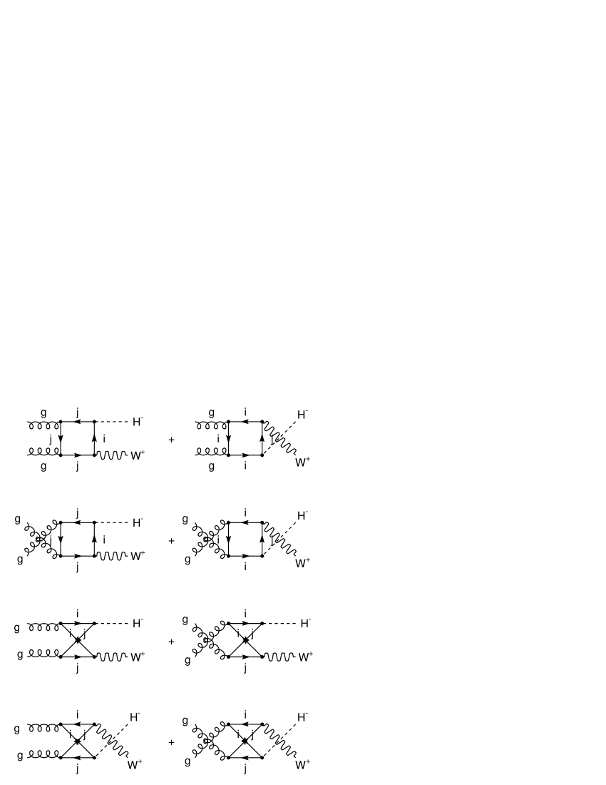
Figure 21: Continued from Figure 20.

8.3 Differential cross section $p\bar{p}\rightarrow H^{\mp}W^{\pm}X$

The differential cross section corresponding to the channel $p\bar{p}\rightarrow H^{\mp}W^{\pm}X$ is:

$$\frac{d^{2}\sigma}{dyd\left(p_{T}\right)^{2}}\left(p\bar{p}\rightarrow H^{\mp}W^{\pm}X\right) = \sum_{f}{\int_{x_{amin}}^{1}{dx_{a}f_{f}\left(x_{a},m_{a}^{2}\right)f_{f}\left(x_{b},m_{b}^{2}\right)}}$$ (67)

$$\times\frac{x_{b}\hat{s}}{\left(m_{H}^{2}-\hat{u}\right)}\frac{d\sigma}{d\hat{t}}\left(f\bar{f}\rightarrow H^{\mp}W^{\pm}\right)$$

where $f$ is $q$ or $g$,

$$x_{amin}=\frac{\sqrt{s}m_{T}e^{y}+m_{H}^{2}-m_{W}^{2}}{s-\sqrt{s}m_{T}e^{-y}},$$ (68)

$$m_{T}=\left(m_{W}^{2}+p_{T}^{2}\right)^{\frac{1}{2}},$$ (69)

$$x_{b}=\frac{x_{a}\sqrt{s}m_{T}e^{-y}+m_{H}^{2}-m_{W}^{2}}{x_{a}s-\sqrt{s}m_{T}e^{y}},$$ (70)

$$\hat{s}=x_{a}x_{b}s,$$ (71)

$$p_{T}^{2}=\frac{\Lambda\left(\hat{s},m_{H}^{2},m_{W}^{2}\right)\sin^{2}\theta}{4\hat{s}},$$ (72)

$$\hat{u}=\frac{1}{2}\left(m_{H}^{2}+m_{W}^{2}-\hat{s}-\cos\theta\Lambda^{1/2}(\hat{s},m_{H}^{2},m_{W}^{2})\right),$$ (73)

$$\hat{t}=\frac{1}{2}\left(m_{H}^{2}+m_{W}^{2}-\hat{s}+\cos\theta\Lambda^{1/2}(\hat{s},m_{H}^{2},m_{W}^{2})\right),$$ (74)

$$\hat{u}\hat{t}=m_{H}^{2}m_{W}^{2}+\hat{s}p_{T}^{2},$$ (75)

and

$$\cos\theta=\left(1-\frac{4\hat{s}p_{T}^{2}}{\Lambda^{1/2}(\hat{s},m_{H}^{2},m_{W}^{2})}\right)^{1/2}$$ (76)

$y$ is the rapidity of $W^{\pm}$, $\theta$ is the angle of dispersion in the center of mass system, $p_{T}$ is the transverse momentum of $W^{\pm}$, $f_{f}$ are the unpolarized parton distribution functions for quarks (antiquarks) or gluons. Finally, $m_{a}^{2}$ or $m_{b}^{2}$ represent the factorization scale.

A similar expression is valid for the reaction $pp\rightarrow H^{\mp}W^{\pm}+X$.

In Figure 22 (taken from reference [11]) the total cross section $\sigma$ of $pp\rightarrow W^{\pm}H^{\mp}+X$ via $b\bar{b}$ annihilation and $gg$ fusion is plotted as a function of $m_{H}$ at LHC energies ($\sqrt{s}=14\textrm{TeV/c}$) for $\tan\beta=30$. Other contributions are negligible.

In Figure 23 (taken from reference [11]) the total cross section $\sigma$ of $p\bar{p}\rightarrow W^{\pm}H^{\mp}+X$ via $b\bar{b}$ annihilation and $gg$ fusion is plotted as a function of $m_{H}$ at the Tevatron energy ($\sqrt{s}=2\textrm{TeV/c}$) for $\tan\beta=30$. The contributions of the other partons are negligible.

Figure 22: Total cross section for the process $pp\rightarrow W^{\pm}H^{\mp}+X$ as a function of $m_{H}$ via $b\bar{b}$ annihilation and $gg$ fusion at LHC energies ($\sqrt{s}=14\textrm{TeV/c}$) for $\tan\beta=30$. Taken from [11].

Figure 23: Total cross section for the process $p\bar{p}\rightarrow W^{\pm}H^{\mp}+X$ as a function of $m_{H}$ via $b\bar{b}$ annihilation and $gg$ fusion at the Tevatron energy ($\sqrt{s}=2\textrm{TeV/c}$) for $\tan\beta=30$. Taken from [11].

9 Comparison between $\mu^{-}\mu^{+}\rightarrow H^{\mp}W^{\pm}$ and $p\bar{p},pp\rightarrow H^{\mp}W^{\pm}X$ for large values of $\tan\beta$

Let us compare the channel $\mu^{-}\mu^{+}\rightarrow H^{\mp}W^{\pm}$ at $\sqrt{s}=500\textrm{GeV/c}$ with the processes $p\bar{p},pp\rightarrow H^{\mp}W^{\pm}X$ at the Tevatron energy ($\sqrt{s}=2\textrm{TeV/c}$) and LHC energies ($\sqrt{s}=14\textrm{TeV/c}$) respectively for large values of $\tan\beta$ (for example $\tan\beta=30$).

At the FNAL energy (Figure 24), we have: $\sigma(\mu^{-}\mu^{+}\rightarrow H^{\mp}W^{\pm})>\sigma(p\bar{p}\rightarrow W^{\pm}H^{\mp}X)$ for $\tan\beta=30$.

At LHC energies (Figure 25), we have: $\sigma(pp\rightarrow W^{\pm}H^{\mp}X)>\sigma(\mu^{-}\mu^{+}\rightarrow H^{\mp}W^{\pm})$ for $\tan\beta=30$.

According to Figure 12, $\sigma(\mu^{-}\mu^{+}\rightarrow H^{\mp}W^{\pm})\gtrsim 5\textrm{fb}$ for $\tan\beta\geq 20$ in the mass interval $100\leq m_{H}\leq 400[\textrm{GeV/c}^{2}]$, which would be an observable number of $H^{\pm}$ for luminosities $>50\textrm{fb}^{-1}$. In the mass region of interest shown in the figures, the dominant decay mode of $H^{\pm}$ is $H^{+}\rightarrow t\bar{b}$ or $H^{-}\rightarrow\bar{t}b$. So the main background would be from $t\bar{t}$ production. Reference [4] shows that such a background overwhelms the charged Higgs boson signal in $p\bar{p}\rightarrow W^{\pm}H^{\mp}X$ at the LHC. In fact, in Section 7 we have shown that $\sigma(\mu^{-}\mu^{+}\rightarrow t\bar{t})\approx 495\textrm{fb}$ for $\sqrt{s}=500\textrm{GeV/c}$. In the LHC the background due to $t\bar{t}$ production is of order [4] 800 pb (three orders of magnitude larger than at a muon collider with $\sqrt{s}=500\textrm{GeV/c}$). At the FNAL energy ($\sqrt{s}=2\textrm{TeV/c}$) something similar happens because $\sigma(p\bar{p}\rightarrow t\bar{t})=5.5\textrm{pb}$ [12].

In the muon collider, the signal of the charged Higgs boson is not overwhelmed.

Then, for large values of $\tan\beta$, the process $\mu^{-}\mu^{+}\rightarrow H^{\mp}W^{\pm}$ is a very attractive channel for the search of $H^{\pm}$ at a $\mu^{-}\mu^{+}$ collider.

Figure 24: Total cross section for the processes $\mu^{-}\mu^{+}\rightarrow H^{\mp}W^{\pm}$ and $p\bar{p}\rightarrow W^{\pm}H^{\mp}+X$ (via $b\bar{b}$ annihilation and $gg$ fusion) as a function of $m_{H}$ at $\sqrt{s}=500\textrm{GeV/c}$ and $\sqrt{s}=2\textrm{TeV/c}$, respectively, for $\tan\beta=30$. Taken partially from [11].

Figure 25: Total cross section for the processes $\mu^{-}\mu^{+}\rightarrow H^{\mp}W^{\pm}$ and $pp\rightarrow W^{\pm}H^{\mp}+X$ (via $b\bar{b}$ annihilation and $gg$ fusion) as a function of $m_{H}$ at $\sqrt{s}=500\textrm{GeV/c}$ and $\sqrt{s}=14\textrm{TeV/c}$, respectively, for $\tan\beta=30$. Taken partially from [11].

10 Conclusions

The discovery of the Standard Model Higgs is one of the principal goals of experimental and theoretical particle physicists. This is because the Higgs mechanism is a cornerstone of the Standard Model. The search for the Standard Model Higgs will also constrain or discover particles of the Two Higgs Doublet Model of type II.

In this paper we have discussed the masses of the Higgs particles in the Two Higgs Doublet Model of type II, and considered the influence of the radiative corrections on these masses. In the absence of radiative corrections, the Higgs boson $h^{0}$ obeys the bound $m_{h^{0}}\leq m_{Z}$. This bound practically has been excluded by the present limits on $m_{h^{0}}$ obtained by LEP and CDF [6]. However, when the radiative corrections are taken into account, $m_{h^{0}}$ increases as the value of $m_{A}$ increases. As a result, we have a new bound: $m_{h^{0}}\leq 128.062\textrm{GeV/c}^{2}$ taking $M_{sb}$ (sbottom mass) and $M_{st}$ (stop mass) of order $1\textrm{TeV/c}^{2}$.

Considering the radiative corrections of the masses, we have calculated

Higgs production cross sections at a muon collider in the Two Higgs Doublet Model of type II. The most interesting production channels are $\mu^{-}\mu^{+}\rightarrow h^{0}Z^{0},H^{0}Z^{0}$ , $H^{-}H^{+},A^{0}Z^{0}$ and $H^{\mp}W^{\pm}$. In the first two channels the radiative corrections of the masses play an important role, which is not true for the other channels. In the reaction $\mu^{-}\mu^{+}\rightarrow h^{0}Z^{0}$, the total cross section becomes important in the mass interval $118\leq m_{h^{0}}\leq 128[\textrm{GeV/c}^{2}]$.

The process $\mu^{-}\mu^{+}\rightarrow A^{0}Z^{0}$, would provide an alternative way for searching the $A^{0}$ looking for peaks in the $b\bar{b}$ distribution. Another interesting channel could be $\mu^{-}\mu^{+}\rightarrow A^{0}h^{0}$. However, this is highly supressed for $m_{A}\geq 200\textrm{GeV/c}^{2}$ because the total cross section is proportional to the factor

$$\cos^{2}\left(\beta-\alpha\right)=\frac{\left(1+\tan\beta\tan\alpha\right)^{2}}{\left(1+\tan^{2}\beta\right)\left(1+\tan^{2}\alpha\right)}$$

(see the Feynman rules given in [9]). This factor decreases as the mass of the $A^{0}$ increases.

The most attractive channel is $\mu^{-}\mu^{+}\rightarrow H^{\mp}W^{\pm}$, see Figures 24 and 25. In this reaction $\sigma(\mu^{-}\mu^{+}\rightarrow H^{\mp}W^{\pm})\gtrsim 5\textrm{fb}$ for $\tan\beta\geq 20$ in the mass interval $100\leq m_{H}\leq 400[\textrm{GeV/c}^{2}]$, which would give an observable number of $H^{\pm}$ for luminosities $>50\textrm{fb}^{-1}$ at $\sqrt{s}=500\textrm{GeV/c}$.

Because the main background in a hadron collider in the reactions $p\bar{p}\rightarrow W^{\pm}H^{\mp}X$ (Tevatron energy) or $pp\rightarrow W^{\pm}H^{\mp}X$ (LHC energies) comes from $t\bar{t}$ production, the charged Higgs boson signal would be overwhelmed by such a background. In a muon collider with $\sqrt{s}=500\textrm{GeV/c}^{2}$, the signal of the $H^{\pm}$ is not overwhelmed. This means, that for large values of $\tan\beta$, the channel $\mu^{-}\mu^{+}\rightarrow H^{\mp}W^{\pm}$ is a very attractive channel for the search of charged Higgs bosons at a $\mu^{-}\mu^{+}$ collider.

References

- [1] Bruce Hoeneisen, Serie de Documentos USFQ , Universidad San Francisco de Quito, Ecuador (2001).
- [2] J. Gunion, hep-ph/9802258; V. Barger, hep-ph/9803480.
- [3] A. G. Akeroyd, A. Arhrib, C. Dove, Phys. Rev. D , 071702 (2000).
- [4] Stefano Moretti, Kosuke Odagiri, Phys. Rev. D , 055008 (1999).
- [5] Vernon Barger and Roger Phillips, Collider Physics (Addison Wesley, 1988); S. Dawson, J.F. Gunion, H.E. Haber and G. Kane, The Higgs Hunter’s Guide (Addison Wesley, 1990).
- [6] Review of Particle Physics, K. Hagiwara et al., Phys. Rev. D , 010001 (2002).
- [7] ”The quantum theory of fields”, Volume III, Supersymmetry, Steven Weinberg, Cambridge University Press (2000).
- [8] Zhou Fei et al., Phys. Rev. D , 055005(2001).
- [9] C. Marín and B. Hoeneisen, hep-ph/0402061 v1 (2004).
- [10] C. Marín, Politécnica, No. 1, p.79 (1992), Escuela Politécnica Nacional, Quito, Ecuador. DO Note Fermilab (1992).
- [11] A. A. Barrientos Bendezú and B. A. Kniehl, Phys. Rev. D , 015009 (1998).
- [12] V. M. Abazov et al., Phys. Rev. Lett. , 151803 (2002).