Minimal left-right symmetric models and new $Z^{\prime}$ properties at future electron-positron colliders

Abstract

It was recently shown that left-right symmetric models for elementary particles can be built with only two Higgs doublets. The general consequence of these models is that the left and right fermionic sectors can be connected by a new neutral gauge boson $Z^{\prime}$ having its mass as the only additional new parameter. In this paper we study the influence of the fundamental fermionic representation for this new neutral gauge boson. Signals of possible new heavy neutral gauge bosons are investigated for the future electron-positron colliders at $\sqrt{s}=500$ GeV , $1$ TeV and $3$ TeV. The total cross sections, forward-backward and left-right asymmetries and model differences are calculated for the process $e^{+}e^{-}\longrightarrow\mu^{+}\mu^{-}$. Bounds on $Z^{\prime}$ masses are estimated.

PACS 12.60.Cn, 14.70.Pw, 14.80.Cp

1 Introduction

One possible way to understand the left-right asymmetry of elementary particles is to enlarge the standard model into a left-right symmetric structure and then, by some spontaneously broken mechanism, to recover the low energy asymmetric world. There are three main points in this proposal: the choice of the gauge group, the Higgs sector and the fundamental fermionic representation.

Left-right models starting from the gauge group $SU(2)_{L}\otimes SU(2)_{R}\otimes U(1)_{B-L}$ were developed by many authors [1] and are well known to be consistent with the standard $SU(2)_{L}\otimes U(1)_{Y}$ model. This group can be part of more general models, like some grand unified groups [2], superstring inspired models [3], a connection between parity and the strong $CP$ problem [4], left-right extended standard models [5]. All these approaches imply the existence of some new intermediate physical mass scale, well bellow the unification or the Planck mass scale.

For the Higgs sector there are some options. Two Higgs doublets that transform as fields in the left and right sectors can be supposed to be spontaneously broken at scales $v_{L}=v_{{Fermi}}$ and at a larger scale $v_{R}$ respectively. The earlier left-right symmetric models added a new Higgs in the mixed representation $(1/2,\,1/2,\,0)$, for $(T_{3L},\,T_{3R},\,Y)$. The symmetry breaking of this field gives a mixing in the charged vector boson sector (not yet experimentally verified) and could also be responsible for neutrino masses. The increasing experimental evidence on neutrino oscillations and nonzero masses has motivated a renewed interest in the mechanisms for parity breaking. More recently it was shown that all fermion masses could be obtained with only two Higgs doublets [6]. The basic mechanism for this model is the dimension-5 operator built by Weinberg years ago [7]. It is also possible to build mirror models with two Higgs doublets and new Higgs singlets [8]. In this case charged fermion masses can be understood as a result of a see-saw mechanism.

Throughout this paper we call models with two Higgs doublets ”minimal models” in the sense that they have the minimal set of new scale parameters that are shown to be consistent with the standard $SU(2)_{L}\otimes U(1)_{Y}$ theory.

For the fermion spectrum there is no unique choice of the fundamental fermionic representation. Earlier left-right models restored parity by choosing the right-handed sector as doublets under $SU(2)_{R}$ with $\nu_{R}$ and $u_{R}$ as the upper components of the right doublet. Other models have doubled the number of fundamental fermions choosing the new sector with opposite chirality relative to the standard model sector.

In this paper we present models that start by the simple gauge structure of $SU(2)_{L}\otimes SU(2)_{R}\otimes U(1)_{B-L}$ and investigate the consequences of the minimal Higgs sector that breaks the left-right symmetry. This paper is organized as follows: in section 2 we review the main assumptions for the Higgs and gauge sector in the minimal left-right model; in section 3 we review the properties of new fermion representation; in section 4 we show some phenomenological consequences for testing the models here proposed and in section 5 we give our conclusions.

2 The Higgs and gauge boson sectors in the minimal model

Left-right models with only two Higgs doublets have been previously considered [6, 8]. We review in this section the main points that are relevant for the new neutral current interactions. The minimal left-right symmetric model contains the following Higgs scalars:

$$\begin{array}[]{ccc}&\chi_{L}=\left(\begin{array}[]{cc}\chi_{L}^{+}\\ \chi_{L}^{0}\end{array}\right),&\chi_{R}=\left(\begin{array}[]{cc}\chi_{R}^{+}\\ \chi_{R}^{0}\end{array}\right),\end{array}$$ (6)

with transformation properties under $SU(2)_{L}\times SU(2)_{R}\times U(1)_{Y}$

$$(1/2,0,1)_{\chi_{L}},\;(0,1/2,1)_{\chi_{R}}.$$ (7)

The first stage of symmetry breaking occurs when $\chi_{R}$ acquires its vacuum expectation value $<\chi_{R}>$, leaving a remnant $U(1)_{Y^{\prime}}$ symmetry coming from the $SU(2)_{R}\times U(1)_{Y}$ sector, whose generator is given by the relation $\frac{1}{2}Y^{\prime}=T_{3R}+\frac{1}{2}Y$, with $Y=B-L$. The breakdown to $U(1)_{em}$ is realized, at the scale $v_{L}\simeq v_{Fermi}$, through the following vacuum expectation value:

$$\begin{array}[]{ccc}&<\chi_{L}>=\left(\begin{array}[]{cc}0\\ v_{L}\end{array}\right).\end{array}$$ (11)

In order to analyze the couplings of the additional neutral gauge boson we rewrite here the free Lagrangian for the gauge fields and the piece containing the covariant derivatives of the scalar fields

$$\mathcal{L} = \mathcal{L}_{0}+\mathcal{L}_{D}$$ (12)

$$\mathcal{L}_{0} = -\frac{1}{4}F^{\mu\nu}F_{\mu\nu}-\frac{1}{2}Tr[G_{L\mu\nu}^{a}G_{L}^{a,\mu\nu}]-\frac{1}{2}Tr[G_{R\mu\nu}^{a}G_{R}^{a,\mu\nu}]$$ (13)

$$\mathcal{L}_{D} = (D_{\mu}\chi_{L})^{\dagger}D^{\mu}\chi_{L}+(D_{\mu}\chi_{R})^{\dagger}D^{\mu}\chi_{R},$$ (14)

where

$$F^{\mu\nu} = \partial^{\mu}B^{\nu}-\partial^{\nu}B^{\mu}$$ (15)

$$G^{a,\mu\nu}_{L,R} = \partial^{\mu}W^{a,\nu}_{L,R}-\partial^{\nu}W^{a,\mu}_{L,R}+ig_{L,R}[W^{a,\mu}_{L,R},W^{a,\nu}_{L,R}],$$ (16)

and

$$D_{\mu}\chi_{L,R} = \partial_{\mu}\chi_{L,R}+ig_{L,R}W_{L,R}\chi_{L,R}.$$ (17)

The gauge coupling constants related to the gauge group $SU(2)_{L}\otimes SU(2)_{R}\otimes U(1)_{B-L}$, are respectively $g_{L}$, $g_{R}$ and $g$. When substituting the vacuum expectation values for the scalar fields in $\mathcal{L}_{D}$, one obtains the gauge bosons mass terms. Explicitly, the mass matrix for the neutral sector in the basis $(W_{L},\,W_{R},\,B)$ is

$$M=\frac{1}{4}\left(\begin{array}[]{ccc}g_{L}^{2}v_{L}^{2}&0&-gg_{L}v_{L}^{2}\\ 0&g_{R}^{2}v_{R}^{2}&-gg_{R}v_{R}^{2}\\ -gg_{L}v_{L}^{2}&-gg_{R}v_{R}^{2}&g^{2}(v_{L}^{2}+v_{R}^{2})\end{array}\right)$$ (21)

The mass matrix $M$ is diagonalized by an orthogonal transformation $R$ which connects the weak fields ($W_{L}^{\mu},\,W_{R}^{\mu},\,B^{\mu}$) to the physical ones ($Z^{\mu},\,Z^{\prime\mu},\,A^{\mu}$). By direct calculation from the neutral mass matrix we can obtain an analytic expression for $R$ in powers of $w=v_{L}/v_{R}$,

$$R=\left(\begin{array}[]{ccc}\cos\theta_{W}&w^{2}\cos\beta\sin^{2}\beta&\sin\theta_{W}\\ -\sin\theta_{W}\sin\beta-\displaystyle{\frac{w^{2}\cos^{2}\beta\sin^{3}\beta}{\sin\theta_{W}}}&\cos\beta-w^{2}\cos\beta\sin^{4}\beta&\sin\beta\cos\theta_{W}\\ -\sin\theta_{W}\cos\beta+\displaystyle{\frac{w^{2}\cos\beta\sin^{4}\beta}{\sin\theta_{W}}}&-\sin\beta-w^{2}\cos^{2}\beta\sin^{3}\beta&\cos\beta\cos\theta_{W}\\ \end{array}\right)$$ (22)

In Eq.(22), the following relations were employed

$$\sin^{2}\theta_{W}=\frac{g^{2}_{R}g^{2}}{\Lambda},\;\;\sin^{2}\beta=\frac{g^{2}}{g_{R}^{2}+g^{2}},\;\;\sin\alpha=\frac{g^{2}\Lambda^{1/2}}{(g_{R}^{2}+g^{2})^{2}}w^{2}+O(w^{3})$$ (23)

with $\Lambda=(g_{L}^{2}g_{R}^{2}+g^{2}g_{L}^{2}+g^{2}g_{R}^{2})$.

In the limit $w=0$, the left and right sectors are decoupled and one recovers the standard model gauge boson couplings. The triple and quartic self-interactions terms contained in the kinetic terms $Tr[G^{\mu\nu}G_{\mu\nu}]_{L,R}$ are explicitly

$$Tr[G^{a,\mu\nu}G^{a}_{\mu\nu}] = \partial^{\mu}W^{a,\nu}\partial_{\mu}W_{\nu}^{a}-\partial^{\nu}W^{a,\mu}\partial_{\mu}W_{\nu}^{a}+2ig_{L,R}f^{abc}\partial^{\mu}W^{a,\nu}W^{b}_{\mu}W^{c}_{\nu}+$$ (24)

$$+ \frac{g^{2}}{2}f^{abc}f^{alm}W^{b}_{\mu}W^{c}_{\nu}W^{l,\mu}W^{m,\nu}$$

where $f^{abc}$ is the totally antisymmetric tensor. Using the mixing matrix $R$ and taking the physical charged fields as being

$$W^{\pm\mu}_{L,R}=\frac{1}{\sqrt{2}}(W_{L,R}^{1\mu}\pm W_{L,R}^{2\mu}),$$ (25)

the Feynman rules for the $W^{+}_{L,R}W^{-}_{L,R}X_{j}$ triple vertices are readily found:

$$\Gamma_{\lambda_{1}\lambda_{2}\lambda_{3}}^{abc}(k_{1},k_{2},k_{3}) = g_{i}R_{ij}f^{abc}[(k_{1}-k_{2})_{\lambda_{3}}g_{\lambda_{1}\lambda_{2}}+(k_{2}-k_{3})_{\lambda_{1}}g_{\lambda_{2}\lambda_{3}}+$$ (26)

$$+ (k_{3}-k_{1})_{\lambda_{2}}g_{\lambda_{3}\lambda_{1}}],$$

with $i=1,\,2$, $g_{1}\equiv g_{L}$, $g_{2}\equiv g_{R}$ and the sub-index $j$ takes the values $1,\,2$ or $3$ whenever $X_{j}$ is identified as $Z$,   $Z^{\prime}$ or $\gamma$ respectively. In Table (1) we summarize the results for the couplings factors $g_{i}R_{ij}$ using the standard parametrization of $R$ in terms of $\sin\theta_{W}(s_{\theta W})$, $\sin\beta(s_{\beta})$ and $sin\alpha(s_{\alpha})$, which correspond to the mixing angles between $Z-A$, $Z^{\prime}-A$ and $Z^{\prime}-Z$ respectively.

Couplings
	$Z$	$Z^{\prime}$	$\gamma$
$W^{+}_{L}W^{-}_{L}$	$g_{L}c_{\theta W}c_{\alpha}$	$g_{L}c_{\theta_{W}}s_{\alpha}$	$g_{L}s_{\theta_{W}}$
$W^{+}_{R}W^{-}_{R}$	$-g_{R}(s_{\alpha}c_{\beta}-c_{\alpha}s_{\theta W}s_{\beta})$	$g_{R}(c_{\beta}c_{\alpha}-s_{\alpha}s_{\theta_{W}}s_{\beta})$	$g_{R}s_{\beta}c_{\theta_{W}}$

Table 1: Triple couplings.

Similarly, for the quartic self-interaction term a straightforward calculation for the $W^{+}_{i}W^{-}_{i}X_{j}X_{k}$ vertex yields the Feynman rules:

$$\Gamma^{abcd}_{\lambda_{1}\lambda_{2}\lambda_{3}\lambda_{4}} = g_{i}^{2}R_{ij}R_{ik}[f^{abe}f^{cde}(g_{\lambda_{1}\lambda_{3}}g_{\lambda_{2}\lambda_{4}}-g_{\lambda_{2}\lambda_{3}}g_{\lambda_{1}}g_{\lambda_{4}})+$$

$$+ f^{ace}f^{bde}(g_{\lambda_{1}\lambda_{2}}g_{\lambda_{3}\lambda_{4}}-g_{\lambda_{3}\lambda_{2}}g_{\lambda_{1}\lambda_{4}})+f^{ade}f^{cbe}(g_{\lambda_{1}\lambda_{3}}g_{\lambda_{2}\lambda_{4}}-g_{\lambda_{4}\lambda_{3}}g_{\lambda 1\lambda_{2}}).$$

The resulting couplings are summarized in Table (2).

Couplings
	$\gamma Z^{\prime}$	Z’Z	Z’Z’
$W_{L}^{+}W_{L}^{-}$	$g_{L}^{2}s_{\theta_{W}}c_{\theta_{W}}s_{\alpha}$	$g_{L}^{2}c^{2}_{\theta_{W}}s_{\alpha}c_{\alpha}$	$g_{L}^{2}c^{2}_{\theta_{W}}s^{2}_{\alpha}$
$W_{R}^{+}W_{R}^{-}$	$g_{R}^{2}s_{\beta}c_{\theta_{W}}$	$g_{R}^{2}(s_{\alpha}c_{\beta}+c_{\beta}s_{\theta_{W}}s_{\beta})(s_{\alpha}s_{\theta_{W}}s_{\beta}-c_{\beta}c_{\alpha})$	$g_{R}^{2}(c_{\beta}c_{\alpha}-s_{\alpha}s_{\theta_{W}}s_{\beta})^{2}$

Table 2: Quartic couplings.

In the high energy limit where the symmetry breaking scales $v_{R}$ and $v_{L}$ can be neglected, the theory is invariant under the parity operation $\cal P$, and we must have $g_{L}=g_{R}$. At lower energies the running couplings lead to different values of $g_{L}$ and $g_{R}$. However, in the region of the $Z^{\prime}$ that we are considering this is a small effect and we will consider $g_{L}=g_{R}$. This simplification reduces the number of the arbitrary gauge coupling to two.

One of the most interesting consequences of the minimal left-right symmetric model is that there is only one new scale parameter in the model, $v_{R}$, besides the usual standard model inputs.

3 Models for the fermion representation

We present in this paper two possibilities for the fundamental fermionic representation.

3.1 Mirror left-right model

In this model [8] (from now on called MLRM) we have new heavy fermions with opposite chirality relative to the present known fermions. The parity operation transforms the $SU(2)_{L}\buildrel{\rm P}\over{\longleftrightarrow}SU(2)_{R}$ sectors, including the vector gauge bosons. For the other leptonic and quark families a similar structure is proposed. The charge generator is given by $Q=T_{3L}+T_{3R}+Y/2$.

The fundamental representation for leptons in this model is:

$${\ell}_{L}={{\nu\choose e}_{L},\qquad\nu_{R},\qquad e_{R},\qquad L_{R}={N\choose E}_{R}},\qquad N_{L},\qquad E_{L}$$ (1)

For quarks we have,

$${u}_{L}={{u\choose d}_{L},\qquad u_{R},\qquad d_{R},\qquad U_{R}={U\choose D}_{R}},\qquad U_{L},\qquad D_{L}.$$ (2)

States	$T_{3L}$	$T_{3R}$	$Y/2$	$Q$
$\nu_{L}$	$1/2$	$0$	$-1/2$	$0$
$e_{L}$	$-1/2$	$0$	$-1/2$	$-1$
$N_{R}$	$0$	$1/2$	$-1/2$	$0$
$E_{R}$	$0$	$-1/2$	$-1/2$	$-1$
$u_{L}$	$1/2$	$0$	$1/6$	$2/3$
$d_{L}$	$-1/2$	$0$	$1/6$	$-1/3$
$U_{R}$	$0$	$1/2$	$1/6$	$2/3$
$D_{R}$	$0$	$-1/2$	$1/6$	$-1/3$

Table 3: Quantum numbers for left and right states in mirror left-right model.

The quantum numbers for this model are shown in Table (3) with the charge operator given by $Q=I_{3L}+I_{3R}+\displaystyle{{B-L}\over 2}$

Introducing the notation

$$sin^{2}\theta_{W} \equiv {{g^{2}_{R}g^{\prime 2}}\over{g^{2}_{R}g^{2}_{L}+g^{2}_{R}g^{\prime 2}+g^{2}_{L}g^{\prime 2}}}$$

$$sin^{2}\beta \equiv {{g^{\prime 2}}\over{g^{2}_{R}+g^{\prime 2}}},$$ (3)

the condition $g_{L}=g_{R}$ implies

$$\sin\beta=\tan\theta_{W}$$ (4)

and the unification condition for the electromagnetic interaction is the same as in the standard model,

$$e=g_{L}\sin\theta_{W}.$$ (5)

We are interested in interactions between the extra neutral gauge boson $Z^{\prime}$ and the ordinary fermions, that are described by the Lagrangian for the neutral currents with $Z$ and $Z^{\prime}$ boson contributions,

$${\cal L_{NC}}= \frac{e}{4\sin\theta_{W}\cos\theta_{W}}\bar{\Psi}_{i}\gamma^{\mu}\{T_{3L}\frac{(1-\gamma_{5})}{2}-Q\sin^{2}\theta_{W}\}\Psi_{i}Z_{\mu}$$

$$+ \frac{e\tan\theta_{W}\tan\beta}{4\sin\theta_{W}}\bar{\Psi}_{i}\gamma^{\mu}\{T_{3L}\frac{(1-\gamma_{5})}{2}-Q\}\Psi_{i}Z^{\prime}_{\mu}.$$ (6)

The couplings between the gauge neutral bosons and the matter fields are explicitly shown in Table (4).

In this model the charged fermion masses can also be understood as having its origin in a see-saw mechanism. This new result comes from the choice of the fundamental fermionic representation and from new Higgs singlets that do not contribute to the gauge boson masses [8].

Couplings	$g_{V}$	$g_{A}$
$Z\nu\nu$	$1$	$1$
$Zee$	$-1+4sin\theta_{W}$	$1$
$Zuu$	$3-8sin\theta_{W}$	$-3$
$Zdd$	$-3+4sin\theta_{W}$	$3$
Couplings	$g^{\prime}_{V}$	$g^{\prime}_{A}$
$Z^{\prime}\nu\nu$	$1$	$(cos^{2}\theta_{W}-sin^{2}\theta_{W})$
$Z^{\prime}ee$	$-1+sin^{2}\theta_{W}$	$(cos^{2}\theta_{W}-sin^{2}\theta_{W})$
$Z^{\prime}uu$	$3-8sin^{2}\theta_{W}$	$+3(cos^{2}\theta_{W}-sin^{2}\theta_{W})$
$Z^{\prime}dd$	$-3+4sin^{2}\theta_{W}$	$-3(cos^{2}\theta_{W}-sin^{2}\theta_{W})$

Table 4: Couplings between the neutral gauge bosons $Z$ and $Z^{\prime}$ and the ordinary fermions in mirror left-right model (first family).

3.2 Symmetric left-right model

In this model (from now on called SLRM) a new right handed fermionic sector appears as a doublet under the $SU(2)_{R}$ transformation [1].

The fundamental representation for leptons and quarks of the gauge group $SU(2)_{L}\otimes SU(2)_{R}\otimes U(1)_{B-L}$ is:

$${\Psi_{L}={\nu\choose e}_{L}\qquad,\qquad\Psi_{R}={N_{e}\choose e}_{R}}$$ (7)

$${q_{L}={u\choose d}_{L}\qquad,\qquad q_{R}={u\choose d}_{R}}$$ (8)

and the quantum numbers are given in Table (5).

States	$I_{3L}$	$I_{3R}$	$(B-L)/2$	$Q$
$\nu_{L}$	$1/2$	$0$	$1/2$	$0$
$e_{L}$	$-1/2$	$0$	$1/2$	$-1$
$N_{eR}$	$0$	$1/2$	$1/2$	$0$
$e_{R}$	$0$	$-1/2$	$1/2$	$-1$
$u_{L}$	$1/2$	$0$	$1/6$	$2/3$
$d_{L}$	$-1/2$	$0$	$1/6$	$-1/3$
$u_{R}$	$0$	$1/2$	$1/6$	$2/3$
$d_{R}$	$0$	$-1/2$	$1/6$	$-1/3$

Table 5: Quantum numbers for left and right states in symmetric left-right model.

Couplings	$g_{V}$	$g_{A}$
$Z\nu\nu$	$1$	$-1$
$Zee$	$-1+4sin\theta_{W}$	$1$
$Zuu$	$3-8sin\theta_{W}$	$-3$
$Zdd$	$-3+4sin\theta_{W}$	$3$
Couplings	$g^{\prime}_{V}$	$g^{\prime}_{A}$
$Z^{\prime}\nu\nu$	$1$	$-1$
$Z^{\prime}ee$	$3$	$1$
$Z^{\prime}uu$	$-5$	$-3$
$Z^{\prime}dd$	$1$	$3$

Table 6: Couplings between the neutral gauge bosons $Z$ and $Z^{\prime}$ and the ordinary fermions in symmetric left-right model (first family).

We can rewrite the gauge couplings in terms of a mixing angle as

$$g=\frac{e}{\sin\theta_{W}}$$ (9)

and

$$g^{\prime}=\frac{e}{\sqrt{\cos 2\theta_{W}}}.$$ (10)

The neutral current Lagrangian that describes the interactions between the ordinary matter with $Z$ and $Z^{\prime}$ boson contributions is

$${\cal L_{NC}} = \frac{e}{4\sin\theta_{W}\cos\theta_{W}}\bar{\Psi}_{i}\gamma^{\mu}\{(1-\gamma_{5})I_{3_{L}}-Q\sin^{2}\theta_{W}\}\Psi_{i}Z_{\mu}$$ (11)

$$+ \frac{e}{\sin\theta_{W}\cos\theta_{W}}\frac{1}{\sqrt{\cos 2\theta_{W}}}\bar{\Psi}_{i}\gamma^{\mu}\{\sin^{2}\theta_{W}(I_{3L}\frac{(1-\gamma_{5})}{2}-Q\sin^{2}\theta_{W})$$

$$+ \cos^{2}\theta_{W}(I_{3R}\frac{(1+\gamma_{5})}{2}-Q\sin^{2}\theta_{W})\}\Psi_{i}Z^{\prime}_{\mu}$$

and the resulting couplings are shown in Table (6).

Couplings
Models	$g^{\prime}_{V}$	$g^{\prime}_{A}$	$g^{\prime}_{V}/g^{\prime}_{A}$
SLRM	-0.08	-0.54	0.15
MLRM	3	1	3

Table 7: Couplings $g^{\prime}_{V}$ and $g^{\prime}_{A}$ of a new $Z^{\prime}$ in mirror left-right model (MLRM) and symmetric left-right model (SLRM) and the ratio $g^{\prime}_{V}/g^{\prime}_{A}$ in both models. ($\sin^{2}\theta_{W}=0.23$).

Couplings
	$Z^{\prime 2}$	$Z^{\prime}Z$	$Z^{\prime}A$
$\chi^{02}_{R}$	$(gR_{22}+g^{\prime}R_{32})^{2}$	$2g^{2}R_{21}R_{22}+2g^{\prime 2}R_{31}R_{32}$	$2g^{2}R_{22}R_{32}+2g^{\prime 2}R_{32}R_{33}$
		$-2g^{\prime}g(R_{22}R_{31}+R_{32}R_{21})$	$-2gg^{\prime}(R_{22}R_{33}+R_{32}R_{33})$
$\chi^{02}_{L}$	$0$	$-2gg^{\prime}R_{11}R_{32}$	$-2gg^{\prime}R_{13}R_{32}$

Table 8: Couplings between scalar and gauge bosons.

In Table (7) we show the most important difference between the two models: the coupling of a new $Z^{\prime}$ and ordinary charged leptons. The MLRM coupling is dominantly axial, whereas the SLRM is dominantly vectorial. This property will give different asymmetries, as will be shown in the next section.

The Particle Data Group, in its 2002 edition [9], summarizes the present data from low energy lepton interaction, lepton-hadron collisions and the high precision data from LEP and SLAC. They also present the experimental averages for the $g_{V}$ and $g_{A}$ couplings for charged and neutral leptons. The most stringent bounds come from the effective coupling of the Z to the electron neutrino, $g_{exp}^{\nu e}=0.528\pm 0.085$ and $\Gamma^{inv}_{exp}(Z)=499.0\pm 1.5$ MeV, to be compared with the standard model predictions $g_{SM}=0.5042$ and $\Gamma^{inv}_{SM}(Z)=501.65\pm 0.15$ MeV. For the muon neutrino coupling with the $Z$ boson, the Particle Data Group quotes $g_{exp}^{\nu\mu}=0.502\pm 0.017$. We have performed a fit to these data, using the standard model predictions, and we find that deviations from the standard model must be bounded, at $95\%$ confidence level by:

$$(\omega^{2}\sin^{4}\beta)<10^{-4}.$$ (12)

This bound is consistent with the present experimental constraint on the $\rho$ parameter. With the value for $\sin\beta$ given in equation (3.3), we have the bound

$$v_{R}>30\,v_{L}.$$ (13)

For the new $Z^{\prime}$ mass we have

$$M_{Z^{\prime}}>800\quad GeV$$ (14)

and the $Z^{\prime}$ mass is the only new unknown parameter.

This value is a little above the present experimental bounds on new gauge bosons searches done by the CDF and DZero collaborations [10] at Fermilab.

The $Z^{\prime}$ total width in MLRM is $\Gamma_{Z^{\prime}}\simeq 6.80\times 10^{-3}M_{Z^{\prime}}$ and $\Gamma_{Z^{\prime}}\simeq 2.15\times 10^{-2}M_{Z^{\prime}}$ in SLRM, 3 times larger than the previous model. The new $Z^{\prime}$ decays can have contributions from many channels. For the channels $Z^{\prime}\longrightarrow f\bar{f}$ with $"f"$ any of the presently known fermions we can compute all the decay ratios using Tables (4) and (6). A second group of decay channels comes from the triple and quartic vertices from Tables (1) and (2). All these channels give small contributions relative to the fermionic channels. The same suppression is present in the scalar and neutral gauge bosons couplings as shown in Table (8). For example, the decay $Z^{\prime}\longrightarrow Z+\chi_{L}+\chi_{L}$ with $M_{\chi_{L}}=150$ GeV has a partial width $\Gamma_{Z^{\prime}}=2.46\times 10^{-3}$ GeV for $M_{Z^{\prime}}=800$ GeV and $\Gamma_{Z^{\prime}}=2.67\times 10^{-1}$ GeV for $M_{Z^{\prime}}=3$ TeV. In mirror models we can have new heavy fermions coupled to the new neutral current. These new exotic channels can have important phase suppression factors depending on their masses. Since these contributions depend on unknown parameters, we will not take them into account.

4 Results

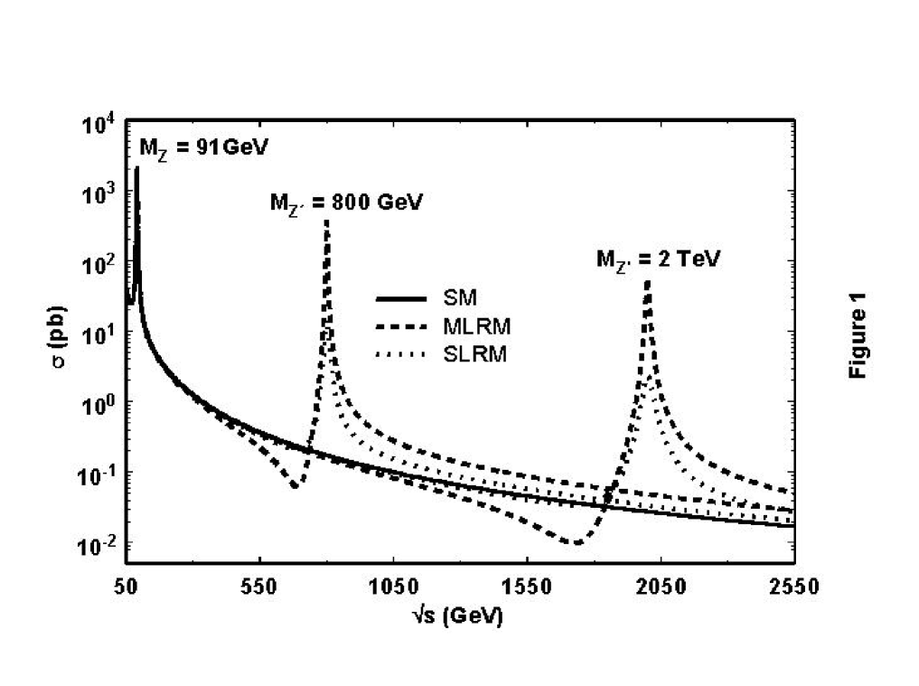
Figure 1: Total cross sections for muon pair production ${e^{+}}{e^{-}}\longrightarrow\mu^{+}\mu^{-}$ versus ${\sqrt{s}}$ for standard model (SM), mirror left-right model (MLRM) and symmetric left-right model (SLRM).

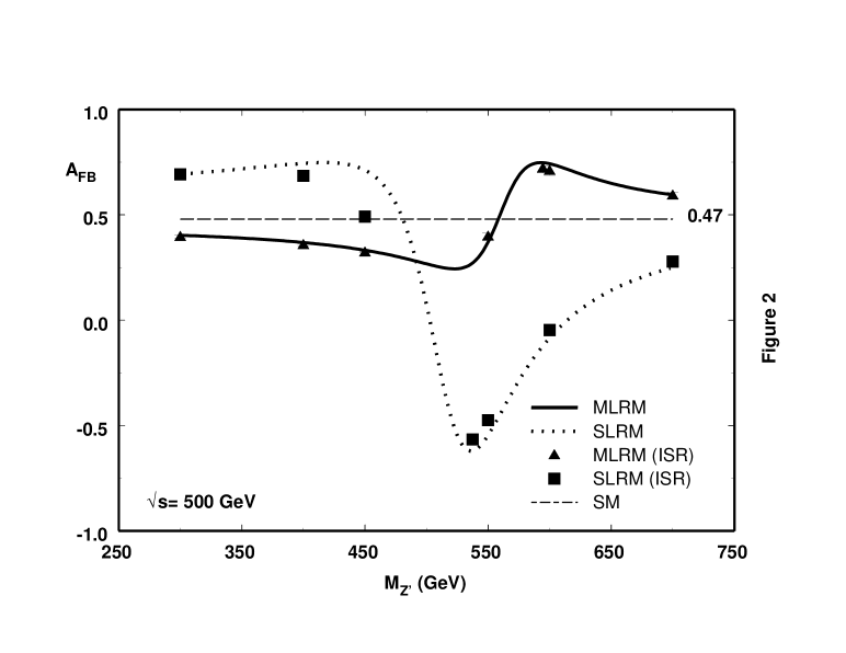
Figure 2: The forward-backward asymmetry in the process ${e^{+}}{e^{-}}\longrightarrow\mu^{+}\mu^{-}$ for SM, SLRM and MLRM versus $M_{Z^{\prime}}$ for TESLA ($\sqrt{s}=500$ GeV).

In this section we present the total cross sections, angular distributions and asymmetries for muon pair production in $e^{+}e^{-}$ annihilation, comparing the signals from MLRM and SLRM with the standard model (SM) background. A Monte Carlo program was written to generate events at a fixed c.m. energy $\sqrt{s}$. To be more specific, three energy values are considered in this paper, $500$ GeV, $1$ TeV and $3$ TeV, which are appropriate for the TESLA at DESY, NLC at SLAC [12] and CLIC at CERN [11] respectively. In these high-energy colliders, the incoming electrons and positrons radiate photons, giving rise to the so-called initial state radiation (ISR), which leads to an effective energy of the annihilation process smaller than the nominal c.m. energy of the colliding beams. In order to correct for ISR, the actual cross sections are written as convolutions of the Born cross sections for muon-pair production, with structure functions for the incoming electron and positron beams. For these structure functions we follow the prescription of reference [13]. The simulated events were selected by a cut $\theta_{acol}<10^{\circ}$ on the acollinearity angle of the final-state muons, which are no longer produced back-to-back on account of ISR. Both muons were also required to be detected within the polar angle range $|\cos{\theta}|<0.995$, where $\theta$ is the angle of either of the muons with respect to the direction of the electron beam. For the numerical calculations, we used $M_{Z}=91.1874$ GeV, $\Gamma_{Z}=2.496$ GeV, $\alpha(M_{Z}^{2})=1/128.5$ and $\sin^{2}{\theta}_{W}=0.23105$. Fermion masses were set to zero. All the calculations involving unpolarized beams were cross-checked with CompHEP [14].

Figure 3: The forward-backward asymmetry in the process ${e^{+}}{e^{-}}\longrightarrow\mu^{+}\mu^{-}$ for SM, SLRM and MLRM versus $M_{Z^{\prime}}$ for NLC ($\sqrt{s}=1$ TeV).

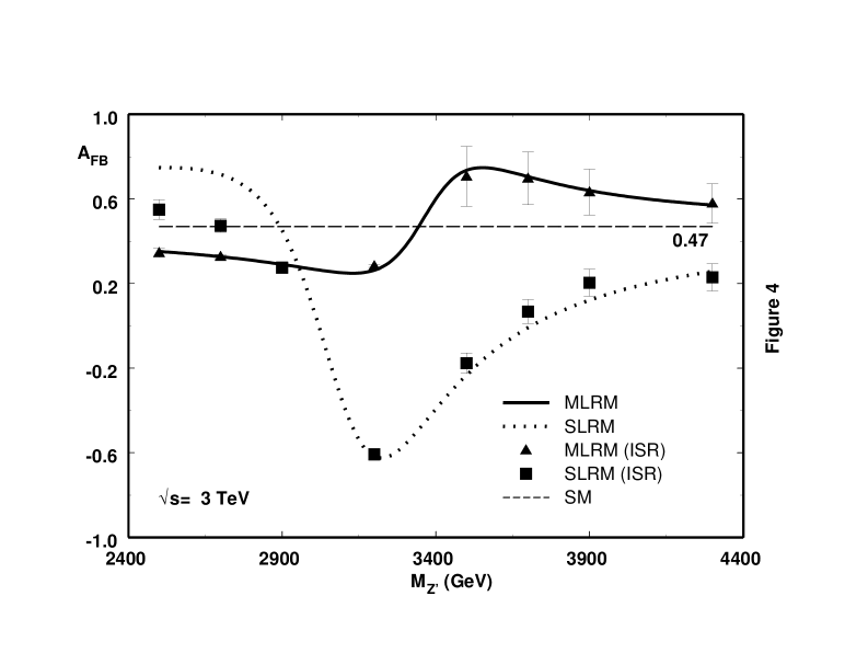
Figure 4: The forward-backward asymmetry in the process ${e^{+}}{e^{-}}\longrightarrow\mu^{+}\mu^{-}$ for SM, SLRM and MLRM versus $M_{Z^{\prime}}$ for CLIC ($\sqrt{s}=3$ TeV).

In Figure 1 we show the total cross section without ISR for the process $e^{+}+e^{-}\longrightarrow\mu^{+}+\mu^{-}$, as a function of the c.m. energy, for SLRM and MLRM. The SM cross section is also shown for comparison. Two different values of $M_{Z^{\prime}}$ are considered, namely $M_{Z^{\prime}}=800$ GeV and $M_{Z^{\prime}}=2$ TeV. The expected resonance peaks associated with these $M_{Z^{\prime}}$ values are clearly shown in the picture, as well as the $Z^{0}$ SM peak. It is interesting to note that the peaks of the MLRM cross sections are greater than those of the SLRM cross sections, because the $Z^{\prime}$ total width is smaller in the MLRM. This property can be used to distinguish the two models. The presence of the new neutral boson $Z^{\prime}$ is essential to preserve tree-level unitarity in both extended models, leading to cross sections that fall to zero for asymptotically high energies.

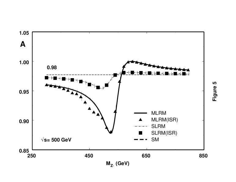
Figure 5: The asymmetry ${\cal A}(P_{-},P_{+})$ in the process ${e^{+}}{e^{-}}\longrightarrow\mu^{+}\mu^{-}$ for SM, SLRM and MLRM versus $M_{Z^{\prime}}$ for TESLA ($\sqrt{s}=500$ GeV). The longitudinal polarization of the electron and positron beams were taken to be $-90\%$ and $60\%$ respectively.

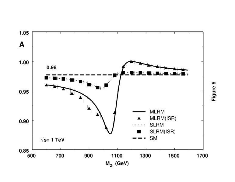
Figure 6: The asymmetry ${\cal A}(P_{-},P_{+})$ in the process ${e^{+}}{e^{-}}\longrightarrow\mu^{+}\mu^{-}$ for SM, SLRM and MLRM versus $M_{Z^{\prime}}$ for NLC ($\sqrt{s}=1$ TeV). The longitudinal polarization of the electron and positron beams were taken to be $-90\%$ and $60\%$ respectively.

Next we look at the dependence of the forward-backward asymmetry $A_{FB}$ on $M_{Z^{\prime}}$. Figures 2, 3 and 4 show the corresponding curves for the collider energies $500$ GeV, $1$ TeV and $3$ TeV respectively, and the points indicate how the ISR affects the asymmetry. In each case the error bars represent the statistical errors for an integrated luminosity of $500$ fb^-1. The forward-backward asymmetry is quite sensitive to $M_{Z^{\prime}}$, and can also be used to distinguish MLRM from SLRM.

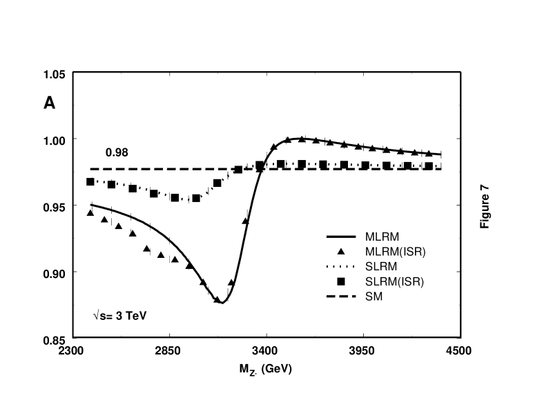
Figure 7: The asymmetry ${\cal A}(P_{-},P_{+})$ in the process ${e^{+}}{e^{-}}\longrightarrow\mu^{+}\mu^{-}$ for SM, SLRM and MLRM versus $M_{Z^{\prime}}$ for CLIC ($\sqrt{s}=3$ TeV). The longitudinal polarization of the electron and positron beams were taken to be $-90\%$ and $60\%$ respectively.

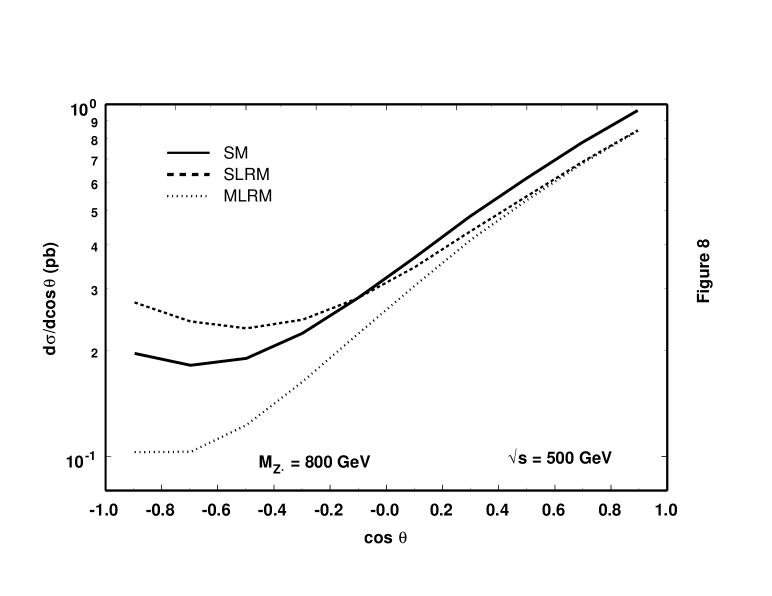
Figure 8: Angular distributions of the $\mu^{-}$ in the process ${e^{+}}{e^{-}}\longrightarrow\mu^{+}\mu^{-}$ for SM, SLRM and MLRM considering $M_{Z^{\prime}}=800$ GeV, $P_{-}=-90\%$ and $P_{+}=60\%$ for TESLA ($\sqrt{s}=500$ GeV).

Beam polarization is expected to play a very important role at the future linear collider facilities. With longitudinally polarized electron and positron beams one can effectively enhance the signals of interest, and suppress inconvenient backgrounds, and thus increase the sensitivity of spin-dependent observables to deviations from the SM predictions. Experts usually believe that it should not be too difficult to produce electron beams whose degrees of polarization exceed $90\%$. As a matter of fact, electron beam polarization routinely reaches values around $80\%$ at SLAC. Several schemes have been devised to produce polarized positron beams in a linear collider. Although these techniques remain untested, simulations suggest that it is feasible to reach a degree of positron polarization of $60\%$. In all the calculations considered in the following, the degrees of polarization of the electron and positron beams were taken to be $P_{-}=-90\%$ and $P_{+}=60\%$ respectively. To illustrate the importance of beam polarization, it suffices to say that for $\sqrt{s}=500$ GeV, the polarized cross section $\sigma(P_{-},P_{+})=\sigma(-0.9,0.6)$ is essentially double the unpolarized cross section $\sigma(0,0)$ . Here we define an asymmetry ${\cal{A}}(P_{-},P_{+})$, in terms of the degrees of polarization $P_{\pm}$ of the electron and positron beams, and the helicity cross sections:

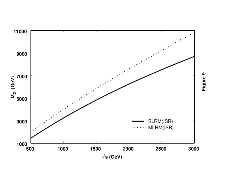
Figure 9: $Z^{\prime}$ mass bound with $95\%$ C.L. as a function of $\sqrt{s}$ for MLRM and SLRM.

$${\cal{A}}(P_{-},P_{+})=\displaystyle\frac{(1-P_{-})(1+P_{+})\sigma_{-+}-(1+P_{-})(1-P_{+})\sigma_{+-}}{(1-P_{-})(1+P_{+})\sigma_{-+}+(1+P_{-})(1-P_{+})\sigma_{+-}}\quad,$$ (15)

where the first (second) subscript in $\sigma_{\pm\mp}$ refers to the electron (positron) helicity. The parity violating left-right asymmetry $A_{LR}=(\sigma_{L}-\sigma_{R})/(\sigma_{L}+\sigma_{R})$ can be easily obtained from $\cal{A}(P_{-},P_{+})$ through the relation

$$A_{LR}=\displaystyle\frac{{\cal{A}}(P_{-},P_{+})-P_{eff}}{1-P_{eff}\cdot{\cal{A}}(P_{-},P_{+})}\quad,$$ (16)

with the effective polarization defined as $P_{eff}=(P_{+}-P_{-})/(1-P_{-}P_{+})$.

Figures 5, 6 and 7 display the behavior of $\cal{A}(-0.9,0.6)$ as a function of $M_{Z^{\prime}}$, for the three energies under study. The differences between MLRM and SLRM asymmetries are considerable, the more so in the resonance region, the deviations from the SM value being larger for the MLRM over the whole $M_{Z^{\prime}}$ range. As expected, the asymmetries in both models tend to the standard model value for $M_{Z^{\prime}}\gg\sqrt{s}$. If we take into account the lower bound in Equation (3.14), $M_{Z^{\prime}}>800$ GeV, it seems unlikely that $\cal{A}(P_{-},P_{+})$ can be used as a measure of the deviations of these models from the SM at the first stage of TESLA, in which $\sqrt{s}\leq 500$ GeV. For a possible TESLA extension, where the c.m. energy could reach $800$ GeV, detection of these deviations in ${\cal{A}}(P_{-},P_{+})$ can not be excluded if $M_{Z^{\prime}}$ is close to the lower bound. For higher values of $\sqrt{s}$, as those of NLC (stage 2) and CLIC, ${\cal{A}}(P_{-},P_{+})$ is sensitive to larger values of the $Z^{\prime}$ boson mass, as long as we exclude the asymptotic region $M_{Z^{\prime}}\gg\sqrt{s}$.

In order to determine the discovery limits for a $Z^{\prime}$ boson via muon pair production, we compared the angular distribution $d\sigma/d(cos\theta)$ predicted by each of the left-right models with the corresponding SM expectation. Plots of the angular distribution are shown in Figure 8 for the extended models and SM, considering $M_{z^{\prime}}=800$ GeV, $P_{-}=-90\%$ and $P_{+}=60\%$ for $\sqrt{s}=500$ GeV. Assuming that the experimental data in muon pair production will be well described by the standard model predictions, we defined a one-parameter $\chi^{2}$ estimator

$$\chi^{2}(\xi)=\sum_{i=1}^{n_{b}}{\biggl{(}{N_{i}^{SM}-N_{i}^{LR}\over\Delta N_{i}^{SM}}\biggr{)}^{2}},$$ (17)

where $N_{i}^{SM}$ is the number of SM events collected in the $i^{th}$ bin, $N_{i}^{LR}$ is the number of events in the $i^{th}$ bin as predicted by the extended model, and $\Delta N_{i}^{SM}=\sqrt{(\sqrt{N_{i}^{SM}})^{2}+(N_{i}^{SM}\epsilon)^{2}}$ the corresponding total error, which combines in quadrature the Poisson-distributed statistical error with the systematic error. We took $\epsilon=5\%$ to correct for those sources of systematic error not explicitly accounted for in our calculation, such as the luminosity uncertainty, beam energy spread and the uncertainty in the muon detection efficiency. The angular range $|cos\,\theta|<0.995$ was divided into $n_{b}=10$ equal-width bins, and the free parameter $\xi=1/M_{Z^{\prime}}$ was varied to determine the $\chi^{2}(\xi)$ distribution. The $95\%$ confidence level bound corresponds to an increase of the $\chi^{2}$ by $3.84$ with respect to the minimum $\chi^{2}_{min}$ of the distribution. Figure 9 represents the $95\%$ confidence limits on the $(\sqrt{s},M_{Z^{\prime}})$ plane for TESLA, NLC and CLIC.

5 Conclusions

We have presented an analysis of the effects of a new neutral gauge boson $Z^{\prime}$ in muon pair production, at the next generation of linear colliders, in the context of two extended electroweak models, the mirror left-right model (MLRM) and the symmetric left-right model (SLRM). A number of observables that are sensitive to the presence of such a gauge boson were studied in detail. These observables were found to be useful to distinguish the two models, should new physics associated with the $Z^{\prime}$ turn up at high mass scales. Our simulations indicate that longitudinally polarized electron and positron beams can significantly increase event rates and the sensitivity of these observables to the presence of a new neutral gauge boson. Starting from the angular distributions of the final $\mu^{-}$, $95\%$ C. L. discovery limits on the $Z^{\prime}$ mass were derived for the new linear colliders, in terms of the available c.m. energies.

Acknowledgments: This work was partially supported by the following Brazilian agencies: CNPq and FAPERJ.

References

- [1] J.C. Pati and A. Salam, Phys. Rev. D 10, 275 (1974) ; R.N. Mohapatra and J.C. Pati, Phys. Rev. D 11, 566 (1975) ; G. Senjanovic̆ and R.N. Mohapatra, Phys. Rev. D 12, 1502 (1975) ; R.N. Mohapatra and R.E. Marshak, Phys. Lett. B 91, 222 (1980). An extensive list of references can be found in R.N. Mohapatra and P.B. Pal, ”Massive Neutrinos in Physics and Astrophysics”, World Scientific, Singapore, 1998
- [2] B. Brahmachari and R.N. Mohapatra, Phys. Lett. B 437, 100 (1998)
- [3] Z.G. Berezhiani and R.N. Mohapatra, Phys. Rev. D 52, 6607 (1995)
- [4] S.M. Barr, D. Chang and G. Senjanovic̆, Phys. Rev. Lett. 67, 2765 (1991)
- [5] R. Foot and R.R. Volkas, Phys. Rev. D 52, 6595 (1995)
- [6] B. Brahmachari, E. Ma and U. Sarkar, Phys. Rev. Lett. 91, 011801 (2003)
- [7] S. Weinberg Phys. Rev. Lett. 43, 1566 (1979)
- [8] Y.A. Coutinho, J.A. Martins Simões, C.M. Porto, Eur. Phys. J. C18, 779 (2001) J.A. Martins Simões, Y.A. Coutinho, C.M. Porto, In *Budapest 2001, High Energy Physics* hep 2001/158, [HEP-PH 0108087]; J.A. Martins Simões, J. Ponciano, Eur. Phys. J. direct C 30, 007 (2003)
- [9] Review of Particle Physics, Phys. Rev. D 66, 010001 (2002)
- [10] F. Abe et al., Phys. Rev. Lett. 79, 2191 (1997) ; S. Obachi et al., Phys. Lett. B 385, 471 (1996)
- [11] G.A. Blair, hep-ex/0104044, and references therein
- [12] American Linear Collider Group, hep-ex/0106055 v1
- [13] M. Skrzypek and S. Jadach, Z. Phys. C49, 577 (1991).
- [14] A. Pukhov, E. Boos, M. Dubinin, V. Edneral, V. Ilyin, D. Kovalenko, A. Kryukov, V. Savrin, S. Shichanin and A. Semenov, ”CompHEP”- a package for evaluation of Feynman diagrams and integration over multi-particle phase space. Preprint INP MSU 98-41/542, hep-ph/9908288.