$K^{+}\rightarrow\pi^{+}\nu\bar{\nu}$ and FCNC from non-universal $Z^{\prime}$ bosons

Abstract

Motivated by the E787 and E949 result for $K^{+}\rightarrow\pi^{+}\nu\bar{\nu}$ we examine the effects of a new non-universal right-handed $Z^{\prime}$ boson on flavor changing processes. We place bounds on the tree-level FCNC from $K-\bar{K}$ and $B-\bar{B}$ mixing as well as from the observed CP violation in kaon decay. We discuss the implications for $K\rightarrow\pi\nu\bar{\nu}$, $B\rightarrow X\nu\bar{\nu}$ and $B\rightarrow\tau^{+}\tau^{-}$. We find that the existing bounds allow substantial enhancements in the $K^{+}\rightarrow\pi^{+}\nu\bar{\nu}$ rate, particularly through a new one-loop $Z^{\prime}$ penguin operator.

I Introduction

The experiments E787 and E949 at Brookhaven National Laboratory have detected three events for the rare mode $K^{+}\rightarrow\pi^{+}\nu\bar{\nu}$. Although the statistics are rather limited so far, the collaborations have published a branching ratio $B(K^{+}\rightarrow\pi^{+}\nu\bar{\nu})=(1.57^{+1.75}_{-0.82})\times 10^{-10}$ for E787 Adler:2001xv and $B(K^{+}\rightarrow\pi^{+}\nu\bar{\nu})=(1.47^{+1.30}_{-0.89})\times 10^{-10}$ for the combined E787 and E949 Artamonov:2004hr which is consistent within errors with the standard model prediction $B(K^{+}\rightarrow\pi^{+}\nu\bar{\nu})=(7.2\pm 2.1)\times 10^{-11}$ Buchalla:1995vs ; smz ; Battaglia:2003in but which has a central value roughly twice the standard model expectation.

This potential discrepancy with the SM has already generated much interest in the literature. In extensions of the SM there are new sources for flavor changing neutral currents which can affect the branching ratio for $K^{+}\to\pi^{+}\nu\bar{\nu}$ and reproduce the central value obtained by E787 and E949 smz ; susy ; z ; other .

New interactions that affect predominantly the third generation are a potential type of new physics that can also enter in this context. Since the process occurs in the standard model via an intermediate top-quark loop, and since it is sensitive to all neutrino generations, $K\rightarrow\pi\nu\bar{\nu}$ has the potential to probe for non-standard couplings of the third generation.

Several scenarios for interactions that single out the third generation have been discussed in the literature. Among them topcolor, where the low energy processes mediated by FCNC have already been discussed in Ref. Buchalla:1995dp . Another possibility consists of new gauge interactions for the third generation. One concrete example was developed in Ref. He:2002kn ; He:2003qv where we constructed a class of models with enhanced right-handed interactions for the third generation. These models are motivated by the small disagreement between the standard model and the measured $A_{FB}^{b}$ at LEP Chanowitz:1999jj ; Chanowitz:2001bv . In this paper we will use this example to illustrate how rare modes such as $K\rightarrow\pi\nu\bar{\nu}$ indirectly probe the physics of the third generation. We consider all the low energy FCNC processes that involve third generation leptons. Some of these processes constrain our models and we use them to discuss the implications for the rest.

The models we consider have been described in detail in Ref. He:2003qv . Their distinctive characteristic is a new right-handed interaction that affects predominantly the third family. Models of this type are interesting in general because they provide specific parameterizations for potential new physics in the couplings of the top-quark. These, in turn, are necessary to test the standard model with experiments designed to determine precisely how the top-quark interacts. The specific form of the interactions in the models we consider here is motivated by the apparent anomaly in the measurement of $A^{b}_{FB}$ at LEP.

II The Model

The models discussed are variations of left-right models in which the right-handed interactions single out the third generation. The first two generations are chosen to have the same transformation properties as in the standard model with $U(1)_{Y}$ replaced by $U(1)_{B-L}$,

$$Q_{L}=(3,2,1)(1/3),\;\;\;\;U_{R}=(3,1,1)(4/3),\;\;\;\;D_{R}=(3,1,1)(-2/3),$$

$$L_{L}=(1,2,1)(-1),\;\;\;\;E_{R}=(1,1,1)(-2).$$ (1)

The numbers in the first parenthesis are the $SU(3)$, $SU(2)_{L}$ and $SU(2)_{R}$ group representations respectively, and the number in the second parenthesis is the $U(1)$ charge. For the first two generations this is the same as the $U(1)_{Y}$ charge in the SM and for the third generation it is the usual $U(1)_{B-L}$ charge of LR models.

The third generation is chosen to transform differently,

$$Q_{L}(3)=(3,2,1)(1/3),\;\;\;\;Q_{R}(3)=(3,1,2)(1/3),$$

$$L_{L}(3)=(1,2,1)(-1),\;\;\;\;L_{R}=(1,1,2)(-1).$$ (2)

The correct symmetry breaking and mass generation of particles can be induced by the vacuum expectation values of three Higgs representations: $H_{R}=(1,1,2)(-1)$, whose non-zero vacuum expectation value (vev) $v_{R}$ breaks the group down to $SU(3)\times SU(2)\times U(1)$; and the two Higgs multiplets, $H_{L}=(1,2,1)(-1)$ and $\phi=(1,2,2)(0)$, which break the symmetry to $SU(3)\times U(1)_{em}$.

The relative strength of left- and right-handed interactions is determined by a parameter $\cot\theta_{R}$. In the limit in which this parameter is large, the new right-handed interactions affect predominantly the third generation. The right-handed interactions may have a triplet of gauge bosons or only a $Z^{\prime}$ depending on the model. The $W^{\prime}$ mixes with the $W$ through a mixing angle $\xi_{W}$ which is severely constrained by $b\rightarrow s\gamma$ He:2002kn . The $Z^{\prime}$ will also mix with the $Z$ through a mixing angle $\xi_{Z}$, and this mixing is severely constrained as well. In particular, it was found in Ref. He:2003qv that the measurement of $g_{R\tau}$ at LEPAbbaneo:2001ix implies

$$\cot\theta_{R}\xi_{Z}\leq 10^{-3}$$ (3)

if the new interaction affects the third generation leptons as well as the quarks. One way out of this problem is to extend the models with additional fermions so that the interactions of the $\tau$ and $\nu_{\tau}$ are the same as in the standard model. These extensions are not significantly constrained by $K\rightarrow\pi\nu\bar{\nu}$ or other low energy FCNC processes and we will not discuss them further in this paper.

Alternatively one must demand that the $W-W^{\prime}$ and $Z-Z^{\prime}$ mixing angles be small. A simple way to accomplish this at tree-level has been discussed in Ref He:2003qv . It consists of taking the vevs of the $\phi$ field to be $v_{2}=0$ in the $2-2$ entry and $v_{1}=v$ in the $1-1$ entry. This eliminates $W-W^{\prime}$ mixing. In addition, one can also eliminate $Z-Z^{\prime}$ mixing at tree level by demanding that the vev of $H_{L}$, $v_{L}$, be equal to $v\cot\theta_{R}$.

In Ref. He:2003qv the process $e^{+}e^{-}\rightarrow b\bar{b}$ at LEP-II was used to obtain a lower bound for the mass of the new $Z^{\prime}$ gauge boson for a given $\cot\theta_{R}$. For our present purpose that bound can be approximated by

$$\cot\theta_{R}\tan\theta_{W}\left({M_{W}\over M_{Z^{\prime}}}\right)\sim 1.$$ (4)

Within this framework there are two potentially large sources of FCNC. The first one, through the coupling $\bar{d}_{i}\gamma_{\mu}P_{R}d_{j}Z^{\prime\mu}$ which occurs at tree level and which also receives large one-loop corrections (enhanced by $\cot\theta_{R}$). The processes we discuss will allow us to constrain the right-handed mixing angles that appear in these couplings. There is a second operator responsible for FCNC of the form $\bar{d}_{i}\gamma_{\mu}P_{L}d_{j}Z^{\prime\mu}$. This operator first occurs at one-loop with a finite coefficient that is enhanced by $\cot\theta_{R}$. This operator is present even when there are no FCNC at tree-level. Because it is enhanced by $\cot\theta_{R}$, it can contribute to a low energy FCNC process at the same level as the ordinary electroweak penguins mediated by the $Z$ boson even though $M_{Z^{\prime}}>>M_{Z}$. Both of these operators can give rise to large contributions to $K\rightarrow\pi\nu\bar{\nu}$ and we discuss them separately in what follows.

II.1 Tree Level FCNC

The models contain flavor changing neutral currents at tree level that contribute to $K\rightarrow\pi\nu\bar{\nu}$ as shown in Figure 1.

Figure 1: Tree-level diagrams responsible for (a) $K\rightarrow\pi\nu\bar{\nu}$ and $b\rightarrow(s{\rm~{}or~{}}d)\nu\bar{\nu}$; (b) $K-\bar{K}$ and $B-\bar{B}$ mixing; and (c) CP violation in $K\rightarrow\pi\pi$.

For models in which the third generation lepton couplings are also enhanced, the relevant interactions are He:2003qv ,

$${\cal L}_{Z} = {g\over 2}\tan\theta_{W}(\tan\theta_{R}+\cot\theta_{R})(\sin\xi_{Z}Z_{\mu}+\cos\xi_{Z}Z^{\prime}_{\mu})$$ (5)

$$\cdot \left(\bar{d}_{Ri}\gamma^{\mu}V^{d*}_{Rbi}V^{d}_{Rbj}d_{Rj}-\bar{u}_{Ri}\gamma^{\mu}V^{u*}_{Rti}V^{u}_{Rtj}u_{Rj}+\bar{\tau}_{R}\gamma^{\mu}\tau_{R}-\bar{\nu}_{R\tau}\gamma^{\mu}\nu_{R\tau}\right)$$

In this expression $g$ is the usual $SU_{L}(2)$ gauge coupling, $\theta_{W}$ the usual electroweak angle, $\theta_{R}$ parametrizes the relative strength of the right-handed interactions, $\xi_{Z}$ is the $Z$-$Z^{\prime}$ mixing angle and $V^{u,d}_{Rij}$ are the unitary matrices that rotate the right-handed up-(down)-type quarks from the weak eigenstate basis to the mass eigenstate basis He:2003qv . For $K\rightarrow\pi\nu\bar{\nu}$ Figure 1(a) shows two types of FCNC: one is mediated by ordinary $Z$ exchange and is proportional to $\cot\theta_{R}\xi_{Z}/M_{Z}^{2}$ while the other one, mediated by a $Z^{\prime}$ exchange, is proportional to $\cot^{2}\theta_{R}/M^{2}_{Z^{\prime}}$. Eqs. 3 and 4 indicate that the latter dominates so we will ignore the $Z$-$Z^{\prime}$ mixing from now on and concentrate on the simpler model with $v_{L}=v\cot\theta_{R}$ where $\xi_{Z}=0$ as mentioned above. Notice that the only enhanced couplings to leptons are to $\tau^{\pm}$ and to $\nu_{\tau}$. For this reason other rare processes such as $K_{L}\rightarrow\mu^{+}\mu^{-}$ are not affected in these models.

For large values of $\cot\theta_{R}$, the dominant tree-level operator responsible for $K\rightarrow\pi\nu\bar{\nu}$ and for $b\rightarrow(s{\rm~{}or~{}}d)\nu\bar{\nu}$ is given by

$${\cal L}={g^{2}\tan^{2}\theta_{W}\cot^{2}\theta_{R}\over 4M^{2}_{Z^{\prime}}}V^{d\star}_{Rbi}V^{d}_{Rbj}\bar{d}_{i}\gamma_{\mu}P_{R}d_{j}\ \bar{\nu}_{\tau}\gamma^{\mu}P_{R}\nu_{\tau}+{\rm~{}h.c.~{}}$$ (6)

Similarly, from Figure 1(b), the new $|\Delta F|=2$ tree-level operators contributing to $K-\bar{K}$ and $B-\bar{B}$ mixing are

$${\cal L}=-{g^{2}\tan^{2}\theta_{W}\cot^{2}\theta_{R}\over 4M^{2}_{Z^{\prime}}}\left(V^{d\star}_{Rbi}V^{d}_{Rbj}\right)^{2}\bar{d}_{i}\gamma_{\mu}P_{R}d_{j}\ \bar{d}_{i}\gamma^{\mu}P_{R}d_{j}+{\rm~{}h.c.~{}}$$ (7)

Finally, from Figure 1(c), the new $|\Delta S|=1$ operator contributing to $K\rightarrow\pi\pi$ and to $\epsilon^{\prime}$ is

$${\cal L} = {g^{2}\tan^{2}\theta_{W}\cot^{2}\theta_{R}\over 4M^{2}_{Z^{\prime}}}V^{d\star}_{Rbs}V^{d}_{Rbd}\bar{s}\gamma_{\mu}P_{R}d\$$ (8)

$$\left(V^{u\star}_{Rtu}V^{u}_{Rtu}\bar{u}\gamma^{\mu}P_{R}u-V^{d\star}_{Rbd}V^{d}_{Rbd}\bar{d}\gamma^{\mu}P_{R}d\right)+{\rm~{}h.c.~{}}$$

The phenomenological constraints that exist on flavor changing processes will severely restrict the non-diagonal right-handed mixing angles $V^{d}_{Rij}$ that appear above.

II.2 Effective $\bar{d}_{i}\gamma_{\mu}P_{L}d_{j}\ Z^{\prime}$ operator

A second mechanism to provide a relatively large contribution to $K^{+}\rightarrow\pi^{+}\nu\bar{\nu}$ occurs at one-loop level and is present even when all the flavor changing couplings $V^{d}_{Rij}$ vanish. It is an effective $Z^{\prime}$ penguin interaction resulting from the diagrams (in unitary gauge) shown in Figure 2. The set of diagrams shown corresponds to those that can be enhanced by a large value of $\cot\theta_{R}$ and only arise from the intermediate top-quark in the loop.

Figure 2: One-loop Feynman diagrams generating the $Z^{\prime}$ penguin operator of the form $\bar{d}_{i}\gamma_{\mu}P_{L}d_{j}Z^{\prime\mu}$ in unitary gauge.

The resulting low energy effective interaction is obtained by setting the external momenta to zero in the calculation of the loop diagrams. It can be written as

$${\cal L}_{eff}={g^{3}\over 16\pi^{2}}\tan\theta_{W}\cot\theta_{R}V^{\star}_{ti}V_{tj}I(\lambda_{t},\lambda_{H})\bar{d}_{i}\gamma_{\mu}P_{L}d_{j}\ Z^{\prime\mu}$$ (9)

where $I(\lambda_{t},\lambda_{H})$ is the corresponding Inami-Lim type function. When a third generation lepton pair is attached to the $Z^{\prime}$ a second factor $\cot\theta_{R}$ is introduced. The resulting coupling compensates for the small $M_{Z}/M_{Z^{\prime}}$ ratio and makes this mechanism comparable to the standard $Z$ penguin as follows from Eq. 4.

Additional diagrams involving a second charged scalar that occurs in the models give rise to the operator $\bar{s}\gamma_{\mu}P_{R}dZ^{\prime}$. We do not need to consider them because they are simply one-loop corrections to the couplings already discussed in the previous section.

To compute the function $I(\lambda_{t},\lambda_{H})$ we work in unitary gauge and restrict ourselves to forms of the Yukawa potential in which $b$-quark intermediate states (and flavor changing neutral scalars) do not appear. The vertices needed for this calculation appear either in the appendix or in Ref. He:2003qv . Diagram (a) in Figure 2 is the only one that does not involve additional parameters from the scalar sector of the models, it results in

$$I(\lambda_{t},\lambda_{H})_{a}={\lambda_{t}\over 8}\left[{\lambda_{t}^{2}-2\lambda_{t}+4\over(1-\lambda_{t})^{2}}\log\lambda_{t}-{3\over\lambda_{t}-1}+{1\over 2}-{1\over\hat{\epsilon}}\right].$$ (10)

We have regularized the ultraviolet divergence in dimensional regularization with

$${1\over\hat{\epsilon}}\equiv{2\over 4-n}-\gamma+\log(4\pi)-\log\;\mu^{2}\,.$$ (11)

The remaining diagrams in Figure 2 cancel the divergence and make the overall result finite but they introduce a dependence on the Higgs parameters. For illustration we consider a simplified Yukawa sector detailed in the appendix in which only one Higgs mass appears in the result. We obtain

$$I(\lambda_{t},\lambda_{H}) = {\lambda_{t}\over 8}\left[{-2\lambda_{t}\over(\lambda_{t}-\lambda_{H})^{2}}\left(\lambda_{H}\log\left({\lambda_{t}\over\lambda_{H}}\right)+\lambda_{H}-\lambda_{t}\right)\cot^{2}\theta_{R}\right.$$ (12)

$$+ {\lambda_{H}^{2}(\lambda_{t}^{2}-2\lambda_{t}+4)+3\lambda_{t}^{2}(2\lambda_{t}-2\lambda_{H}-1)\over(\lambda_{t}-1)^{2}(\lambda_{t}-\lambda_{H})^{2}}\log\lambda_{t}$$

$$- {\lambda_{H}(\lambda_{H}^{2}+6\lambda_{t}-7\lambda_{H})\over(\lambda_{H}-1)(\lambda_{t}-\lambda_{H})^{2}}\log\lambda_{H}+\left.{2\lambda_{t}^{2}-3\lambda_{H}\lambda_{t}-5\lambda_{t}+6\lambda_{H}\over(\lambda_{t}-1)(\lambda_{t}-\lambda_{H})}\right].$$

This form factor is shown in Figure 3 for values of $\cot\theta_{R}$ between 3 and 10 and of $M_{H}$ between 400 and 1200 GeV.

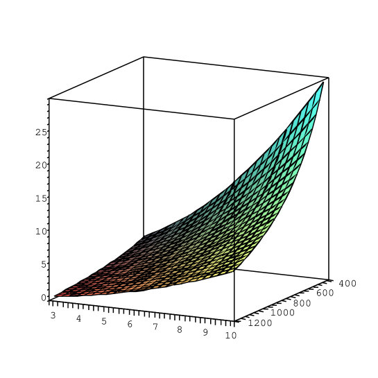
Figure 3: $I(\lambda_{t},\lambda_{H})$ for $\cot\theta_{R}=3{\rm~{}to~{}}10$ and $M_{H}=400{\rm~{}to~{}}1200~{}{\rm GeV}$.

Within this simplified Yukawa sector the new $Z^{\prime}$ penguin has the same flavor dependence as the standard model $Z$ penguin, namely $V^{\star}_{ti}V_{tj}$.

III Constraints from Mixing and CP Violation

III.1 $K-\bar{K}$ Mixing

In many cases tree-level FCNC are severely constrained by $K-\bar{K}$ mixing as in the second diagram of Figure 1. In our models Eq. 6 generates a new contribution to the $K_{L}-K_{S}$ mass difference:

$$\Delta M={g^{2}\tan^{2}\theta_{W}\cot^{2}\theta_{R}\over 4M^{2}_{Z^{\prime}}}{2\over 3}F_{K}^{2}M_{K}B_{K}{\rm Re}\left(V^{d\star}_{Rbs}V^{d}_{Rbd}\right)^{2}.$$ (13)

The calculation of $\Delta M$ in the kaon system is complicated by the existence of long distance contributions. To constrain the new interaction we will require that its contribution to the $K_{L}-K_{S}$ mass difference be at most equal to the largest short distance contribution in the standard model, which is given by Buchalla:1995vs

$$\Delta M\approx{G_{F}^{2}\over 6\pi^{2}}F^{2}_{K}B_{K}M_{K}M_{W}^{2}\left(V^{\star}_{cs}V_{cd}\right)^{2}\eta_{1}{m_{c}^{2}\over M_{W}^{2}}.$$ (14)

In this expression the QCD correction factor $\eta_{1}$ is equal to $1.38$, the kaon decay constant $F_{K}$ and $B_{K}$ are as in the notation of Ref. Buchalla:1995vs . For our numerical estimates we will use the values of the CKM parameters found in Ref. Battaglia:2003in in the Wolfenstein parameterization:

$$\lambda=0.224,\ A=0.839,\ \rho=0.178,\ \eta=0.341$$ (15)

With all this, we obtain a constraint on the right-handed mixing angles

$${\rm Re}\left(V^{d\star}_{Rbs}V^{d}_{Rbd}\right)^{2}\cot^{2}\theta_{R}\tan^{2}\theta_{W}\left({M_{W}\over M_{Z^{\prime}}}\right)^{2}\leq 2.4\times 10^{-8}.$$ (16)

If we further use Eq. 4, and we assume that any new phases are small, this implies that

$${\rm Re}\left(V^{d\star}_{Rbs}V^{d}_{Rbd}\right)\leq 1.5\times 10^{-4}.$$ (17)

III.2 $B-\bar{B}$ Mixing

Similarly we consider the new contributions to mixing in the $B$-sector from Eq. 7. The calculation of $\Delta M$ in the $B_{d}$ system is much more precise than in the kaon system, and the result agrees rather well with the measurement. In this comparison, the dominant uncertainty occurs in the parameters $F_{B_{d}}$ and $B_{B_{d}}$ that occur in the calculation. Following Ref. Battaglia:2003in we write

$$(\Delta M)_{B_{d}}=0.50{\rm~{}ps}^{-1}(1\pm 0.15)^{2},$$ (18)

which corresponds to taking $F_{B_{d}}\sqrt{B_{B_{d}}}=230\pm 35$ MeV, and ignoring all other uncertainties. This is to be compared to the world average $(\Delta M)_{B_{d}}=(0.503\pm 0.006){\rm ps}^{-1}$ Battaglia:2003in . In view of this we will demand that the new physics contribution be smaller than the theoretical uncertainty. With these numbers and Eq. 7 we find,

$$((\Delta M)_{B_{d}})_{new}=\cot^{2}\theta_{R}\tan^{2}\theta_{W}\left({M_{W}\over M_{Z^{\prime}}}\right)^{2}\left|V^{d\star}_{Rbb}V^{d}_{Rbd}\right|^{2}3.2\times 10^{-6}~{}{\rm GeV}\leq 10^{-13}~{}{\rm GeV}.$$ (19)

Once again, we may combine this result with Eq. 4 to find

$$\left|V^{d\star}_{Rbb}V^{d}_{Rbd}\right|\leq 1.8\times 10^{-4}.$$ (20)

For $(\Delta M)_{B_{s}}$ there exists only a lower bound. We first consider the ratio of the new contribution to the standard model where the latter is obtained from the effective Hamiltonian Buchalla:1995vs

$${\cal H}_{SM}={G^{2}_{f}\over 4\pi^{2}}M^{2}_{W}\left(V^{\star}_{tb}V_{ts}\right)^{2}\eta_{2B}S_{0}(x_{t})\ \bar{b}\gamma_{\mu}P_{L}s\ \bar{b}\gamma^{\mu}P_{L}s.$$ (21)

Using $S_{0}(x_{t})\approx 2.56$ and $\eta_{2B}=0.55$ Buchalla:1995vs this results in

$${(\Delta M)_{B_{s}-new}\over(\Delta M)_{B_{s}-SM}}\approx 530\left|{V^{d\star}_{Rbb}V^{d}_{Rbs}\over V^{\star}_{tb}V_{ts}}\right|^{2}\cot^{2}\theta_{R}\tan^{2}\theta_{W}\left({M_{W}\over M_{Z^{\prime}}}\right)^{2}.$$ (22)

We can simplify this further by using $V_{tb}\approx 1$, $V^{d}_{Rbb}\approx 1$ (as discussed in Ref. He:2003qv ), and Eq. 4. The eventual measurement of $B_{s}$ mixing will impact the modes that we discuss next. For this reason it will be convenient to define a parameter $\delta_{B_{s}}$ characterizing the deviation from the standard model prediction $(\Delta M)_{B_{s}}=17.2\ {\rm~{}ps}^{-1}$ Battaglia:2003in ,

$$\delta_{B_{s}}=\left({(\Delta M)_{B_{s}}-17.2{\rm~{}ps}^{-1}\over 17.2{\rm~{}ps}^{-1}}\right).$$ (23)

If we then require the new contribution to explain any deviation from the SM we obtain

$$|V^{d}_{Rbs}|\leq 1.8\times 10^{-3}\ \sqrt{\delta_{B_{s}}}.$$ (24)

Alternatively, we can use $F_{B_{s}}/F_{B_{d}}=1.2$ to write

$${(\Delta M)_{B_{s}-new}\over(\Delta M)_{B_{d}-new}}\approx 1.5\left|{V^{d}_{Rbs}\over V^{d}_{Rbd}}\right|^{2}.$$ (25)

III.3 CP violation in $\epsilon$ and $\epsilon^{\prime}$

We can also place bounds on the phases of the right-handed mixing angles by considering the contributions of Eqs. 7 and 8 to $\epsilon$ and $\epsilon^{\prime}$ respectively. From Eq. 7

$${\rm Im}M_{12}={g^{2}\tan^{2}\theta_{W}\cot^{2}\theta_{R}\over 4M^{2}_{Z^{\prime}}}{2\over 3}F_{K}^{2}B_{K}M_{K}{\rm Im}\left(V^{d\star}_{Rbs}V^{d}_{Rbd}\right)^{2}.$$ (26)

Within the standard model the theoretical uncertainty arises predominantly from $B_{K}$ and is about $30\%$. Consequently we will compare the new contribution to the corresponding expression in the standard model Buchalla:1995vs and demand that

$${\epsilon_{new}\over\epsilon_{SM}}\approx 1.7\times 10^{10}\cot^{2}\theta_{R}\tan^{2}\theta_{W}\left({M_{W}\over M_{Z^{\prime}}}\right)^{2}{\rm Re}\left(V^{d\star}_{Rbs}V^{d}_{Rbd}\right){\rm Im}\left(V^{d\star}_{Rbs}V^{d}_{Rbd}\right)\leq 0.3.$$ (27)

With the aid of Eq. 4 this then implies that

$${\rm Re}\left(V^{d\star}_{Rbs}V^{d}_{Rbd}\right){\rm Im}\left(V^{d\star}_{Rbs}V^{d}_{Rbd}\right)\leq 2\times 10^{-11}.$$ (28)

We turn now to the effect of Eq. 8 on $\epsilon^{\prime}$. In this case there are large theoretical uncertainties and it is best to treat the new contributions as a correction to the result obtained from the standard penguin operator $\epsilon^{\prime}_{6}$. We write

$${\epsilon^{\prime}\over\epsilon}=\left({\epsilon^{\prime}\over\epsilon}\right)_{6}\left(1-\Omega_{SM}-\Omega_{new}\right).$$ (29)

The parameter $\Omega_{new}$ contains the corrections from new physics and we follow Ref. He:1995na to write Eq. 8 as

$${\cal H}_{new}={g^{2}\over\Lambda^{2}}\left(\lambda_{dd}{\cal O}^{(1)}_{dd}-\lambda_{uu}{\cal O}^{(1)}_{ud}\right).$$ (30)

We thus identify $\Lambda=M_{Z^{\prime}}$ and

$$\lambda_{dd} = {\tan^{2}\theta_{W}\cot^{2}\theta_{R}\over 2}\left(V^{d\star}_{Rbs}V^{d}_{Rbd}\right)\left|V^{d}_{Rbd}\right|^{2}$$

$$\lambda_{uu} = {\tan^{2}\theta_{W}\cot^{2}\theta_{R}\over 2}\left(V^{d\star}_{Rbs}V^{d}_{Rbd}\right)\left|V^{u}_{Rtu}\right|^{2}.$$ (31)

Using the results of Ref. He:1995na this leads to

$$\Omega_{new}=4\cot^{2}\theta_{R}\tan^{2}\theta_{W}\left({M_{W}\over M_{Z^{\prime}}}\right)^{2}\left(2.58\left|V^{d}_{Rbd}\right|^{2}+2.52\left|V^{u}_{Rtu}\right|^{2}\right){{\rm Im}\left(V^{d\star}_{Rbs}V^{d}_{Rbd}\right)\over{\rm Im}\left(V^{\star}_{ts}V_{td}\right)}.$$ (32)

We require this correction to be less than one and we use Eq. 4 to obtain

$$\left(\left|V^{d}_{Rbd}\right|^{2}+\left|V^{u}_{Rtu}\right|^{2}\right){\rm Im}\left(V^{d\star}_{Rbs}V^{d}_{Rbd}\right)\leq 1.3\times 10^{-5}.$$ (33)

IV Decays $K\rightarrow\pi\nu\bar{\nu}$

To quantify the new contributions to the rate $K\rightarrow\pi\nu\bar{\nu}$ that occur in these models, it will be convenient to compare them to the dominant standard model amplitude. This one arises from a top-quark intermediate state through the effective Hamiltonian Buchalla:1995vs

$$\tilde{H}_{eff}={G_{F}\over\sqrt{2}}{2\alpha\over\pi\sin^{2}\theta_{W}}V^{\star}_{ts}V_{td}X(x_{t})\bar{s}\gamma_{\mu}P_{L}d\ \sum_{\ell}\bar{\nu_{\ell}}\gamma^{\mu}P_{L}\nu_{\ell}.$$ (34)

In this expression $x_{t}=m_{t}^{2}/M_{W}^{2}$ and the Inami-Lim function $X(x_{t})$ is approximately equal to 1.6 Buchalla:1995vs .

IV.1 $K^{+}\rightarrow\pi^{+}\bar{\nu}\nu$

We first consider the tree-level operator of Eq. 6. Noticing that only the vector current contributes to the $K\rightarrow\pi$ matrix element, that the new interaction couples only to one of the three light neutrino flavors (the $\nu_{\tau}$), and that the right handed nature of the coupling to the neutrino prevents this amplitude from interfering with the SM amplitude, we can write for the rate $\Gamma(K^{+}\rightarrow\pi^{+}\bar{\nu}\nu)$

$$\Gamma_{new}\approx 1130\cot^{4}\theta_{R}\tan^{4}\theta_{W}\left({M_{W}\over M_{Z^{\prime}}}\right)^{4}\left|{V^{d\star}_{Rbs}V^{d}_{Rbd}\over V^{\star}_{ts}V_{td}}\right|^{2}\tilde{\Gamma}_{SM}.$$ (35)

We use the notation $\tilde{\Gamma}_{SM}$ to indicate that this is only the contribution from the top-quark intermediate state. If we use Eq. 4 as well as the constraint from $K-\bar{K}$ mixing (Eq. 17) assuming that the real part dominates, we find that $K^{+}\rightarrow\pi^{+}\bar{\nu}\nu$ can be enhanced by two orders of magnitude with respect to the SM prediction

$$\Gamma_{new}\sim 200\ \tilde{\Gamma}_{SM}.$$ (36)

Of course this result is in gross violation of the experimental observation, implying that the process $K^{+}\rightarrow\pi^{+}\nu\bar{\nu}$ already places a much stronger constraint on these angles than $K-\bar{K}$ mixing does. If we require that the new contribution to $K^{+}\rightarrow\pi^{+}\nu\bar{\nu}$ be at most as large as the standard model (which is needed to match the E787 and E949 central value) we find

$$\left|{V^{d\star}_{Rbs}V^{d}_{Rbd}\over V^{\star}_{ts}V_{td}}\right|^{2}\cot^{4}\theta_{R}\tan^{4}\theta_{W}\left({M_{W}\over M_{Z^{\prime}}}\right)^{4} \leq 8.9\times 10^{-4}{\rm~{}~{}~{}or,}$$

$$\left|V^{d\star}_{Rbs}V^{d}_{Rbd}\right| \leq 1\times 10^{-5}.$$ (37)

At present these models can accommodate the $B(K^{+}\to\pi^{+}\nu\bar{\nu})$ obtained by E787 and E949. However, if we bound $|V_{Rbs}^{d*}V^{d}_{Rbd}|$ by a combination of Eqs. 20 and 24 assuming that $\delta_{B_{s}}$ is at most of order one, we find that this new contribution to $K^{+}\to\pi^{+}\nu\bar{\nu}$ is very small.

After suppressing the tree-level FCNC to a phenomenologically acceptable level, there remains the new one-loop effective interaction of Eq. 9. This effective interaction leads to a correction to $K^{+}\rightarrow\pi^{+}\nu\bar{\nu}$

$$\Gamma_{new}\sim{1\over 12}\cot^{4}\theta_{R}\tan^{4}\theta_{W}\left({M_{W}\over M_{Z^{\prime}}}\right)^{4}\left|{I(\lambda_{t},\lambda_{H})\over X(x_{t})}\right|^{2}\tilde{\Gamma}_{SM}.$$ (38)

Using Eq. 4 and requiring $B(K^{+}\to\pi^{+}\nu\bar{\nu})$ to be twice the SM result (approximately the central value of the measurement) gives

$$I(\lambda_{t},\lambda_{H})=5.54.$$ (39)

From Figure 3 we see that it is possible to obtain this result in our model. In Figure 4 we show two projections of Figure 3 for $M_{H}=1$ TeV and $\cot\theta_{R}=8$. From these we can read off the respective constraints that result from demanding that $I(\lambda_{t},\lambda_{H})\leq 5.54$

$$\cot\theta_{R}\leq 9 {\rm~{}for~{}} M_{H}=1~{}{\rm TeV}$$

$$M_{H}>950~{}{\rm GeV} {\rm~{}for~{}} \cot\theta_{R}=8.$$ (40)

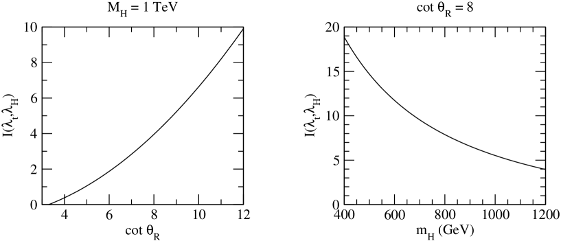
Figure 4: $I(\lambda_{t},\lambda_{H})$ for a) $M_{H}=1$ TeV and b) $\cot\theta_{R}=8$.

The form of this constraint is much more complicated for the most general Yukawa sector. However, it is possible to enhance the $K^{+}\rightarrow\pi^{+}\nu\bar{\nu}$ rate by the factor of two suggested by E787 and E949.

IV.2 $K_{L}\rightarrow\pi^{0}\bar{\nu}\nu$

In this case the rates are sensitive to the CP violating component of the effective interactions. For the tree-level operators

$$\Gamma_{new}\sim 1130\cot^{4}\theta_{R}\tan^{4}\theta_{W}\left({M_{W}\over M_{Z^{\prime}}}\right)^{4}\left({{\rm Im}(V^{d\star}_{Rbs}V^{d}_{Rbd})\over{\rm Im}(V^{\star}_{ts}V_{td})}\right)^{2}\tilde{\Gamma}_{SM}.$$ (41)

Using the current experimental bound $B(K_{L}\rightarrow\pi^{0}\bar{\nu}\nu)<5.9\times 10^{-7}$ Alavi-Harati:1999hd , combined with the standard model prediction (central value) $B(K_{L}\rightarrow\pi^{0}\bar{\nu}\nu)=2.4\times 10^{-11}$ Battaglia:2003in and Eq. 4 results in

$$\left|{\rm Im}\left(V^{d\star}_{Rbs}V^{d}_{Rbd}\right)\right|\leq 6.3\times 10^{-4}.$$ (42)

Alternatively, if we use Eq. 37, assuming that the imaginary part saturates the $K^{+}\rightarrow\pi^{+}\bar{\nu}\nu$ rate, we find

$$B(K_{L}\rightarrow\pi^{0}\bar{\nu}\nu)<1.4\times 10^{-10}.$$ (43)

As mentioned before, the one-loop operator (Eq. 12) has the same phase as the standard model effective Hamiltonian, Eq. 34 and therefore its contribution to $K_{L}\rightarrow\pi^{0}\bar{\nu}\nu$ is rigorously limited by its contribution to $K^{+}\rightarrow\pi^{+}\bar{\nu}\nu$. If this is the only new physics present

$$\Gamma(K_{L}\rightarrow\pi^{0}\bar{\nu}\nu)=\Gamma(K_{L}\rightarrow\pi^{0}\bar{\nu}\nu)_{SM}\left({\Gamma(K^{+}\rightarrow\pi^{+}\bar{\nu}\nu)\over\Gamma(K^{+}\rightarrow\pi^{+}\bar{\nu}\nu)}_{SM}\right).$$ (44)

V Rare B decay modes

The $K$ decay modes discussed in the previous section have obvious extensions to the $B$ sector. In addition to that there are additional modes involving the third generation charged lepton that are also enhanced in the models we discuss. The inclusive modes of the form $B\rightarrow X\tau^{+}\tau^{-}$ receive contributions from an intermediate photon and are less sensitive to the $Z^{\prime}$ operators so we will not discuss them. Additional $B$ decay modes have been considered within the context of FCNC and $Z^{\prime}$ Barger:2003hg . These additional modes involve first and second generation fermions coupling to the $Z^{\prime}$ and for this reason they do not constrain our model significantly.

V.1 $B\rightarrow X_{d,s}\nu\bar{\nu}$

For the modes $B\rightarrow X_{d,s}\nu\bar{\nu}$ the analogue to Eq. 35 for the tree-level FCNC is

$${\Gamma_{new}\over\Gamma_{SM}}\approx 1130\cot^{4}\theta_{R}\tan^{4}\theta_{W}\left({M_{W}\over M_{Z^{\prime}}}\right)^{4}\left|{V^{\star d}_{Rbb}V^{d}_{Rbi}\over V^{\star}_{tb}V_{ti}}\right|^{2}.$$ (45)

For $B\rightarrow X_{d}\nu\bar{\nu}$ we can use the constraint Eq. 20 together with Eq. 4 to see that the additional new contribution does not change the standard model prediction by more than $50\%$. Using the central value $B_{SM}(B\rightarrow X_{d}\nu\bar{\nu})=1.6\times 10^{-6}$ Buchalla:1995vs this implies

$$B(B\rightarrow X_{d}\nu\bar{\nu})\leq 2.4\times 10^{-6}.$$ (46)

Similarly we can use $B_{SM}(B\rightarrow X_{s}\nu\bar{\nu})=4\times 10^{-5}$ Buchalla:1995vs , along with Eqs. 22, 45 to obtain in terms of Eq. 23

$$B(B\rightarrow X_{s}\nu\bar{\nu})\leq 4\times 10^{-5}(1+2\ \delta_{B_{s}}).$$ (47)

At one-loop the form of Eqs.34 and 12 implies that these modes receive identical constraints to Eq 38.

V.2 $B_{i}\rightarrow\tau^{+}\tau^{-}$

Finally the effective Hamiltonian responsible for $B_{i}\rightarrow\tau^{+}\tau^{-}$ within the standard model is Buchalla:1995vs

$${\cal H}=-{G_{F}\over\sqrt{2}}{2\alpha\over\pi\sin^{2}\theta_{W}}V^{\star}_{tb}V_{ti}\ Y(x_{t})\ \bar{b}\gamma_{\mu}P_{L}d_{i}\ \bar{\tau}\gamma^{\mu}P_{L}\tau$$ (48)

where the Inami-Lim function $Y(x_{t})\approx 1.06$ Buchalla:1995vs . Using the central values for hadronic parameters from Ref. Battaglia:2003in this leads to standard model branching ratios $B(B_{s}\rightarrow\tau^{+}\tau^{-})=1.1\times 10^{-6}$ and $B(B_{d}\rightarrow\tau^{+}\tau^{-})=3.3\times 10^{-8}$. The contribution of the tree-level FCNC to the rates, normalized by the standard model rate is

$${\Gamma_{new}\over\Gamma_{SM}}\approx 7730\cot^{4}\theta_{R}\tan^{4}\theta_{W}\left({M_{W}\over M_{Z^{\prime}}}\right)^{4}\left|{V^{\star d}_{Rbb}V^{d}_{Rbi}\over V^{\star}_{tb}V_{ti}}\right|^{2}.$$ (49)

This is somewhat larger than the corresponding ratio for $b\rightarrow d_{i}\nu\bar{\nu}$ because it does not have the factor of $1/3$ that indicates that only the $\nu_{\tau}$ couples strongly to the new interactions and also because $Y(x_{t})$ is slightly smaller than $X(x_{t})$. With the constraints Eqs. 4 and 20 we find that

$$B(B_{d}\rightarrow\tau^{+}\tau^{-})\leq 1.5\times 10^{-7}.$$ (50)

For the $B_{s}$ we resort again to Eq. 23 to write

$$B(B_{s}\rightarrow\tau^{+}\tau^{-})=1.1\times 10^{-6}\left(1+15\ \delta_{B_{s}}\right).$$ (51)

The contribution to these rates from the new penguin operator, relative to their standard model value, is about a factor of 7 larger that its contribution to the $K^{+}\rightarrow\pi^{+}\nu\bar{\nu}$ mode. Again, this factor arises from $Y(x_{t})$ being somewhat smaller than $X(x_{t})$ and because the new operator only couples to $\nu_{\tau}$.

VI Summary and Conclusions

We have examined the effects of a new non-universal right-handed $Z^{\prime}$ boson on several rare flavor changing processes: $K^{+}\to\pi^{+}\nu\bar{\nu}$, $K_{L}\to\pi^{0}\nu\bar{\nu}$, $K-\bar{K}$ and $B-\bar{B}$ mixing, $B\rightarrow X_{d,s}\nu\bar{\nu}$ and $B\rightarrow\tau^{+}\tau^{-}$. There are two mechanisms by which these models can enhance these modes with respect to the standard model.

The first mechanism arises from tree-level FCNC present in the couplings of the non-universal right-handed $Z^{\prime}$ boson. The new $Z^{\prime}$ boson can only have large couplings to third generation leptons and its couplings to the $\tau$ lepton are constrained by LEP. In the quark sector, the flavor conserving couplings of the $Z^{\prime}$ are large only for the $b$ and $t$ quarks. However the flavor changing couplings to the first two generation quarks could be large if the right-handed mixing angles are large. In this paper we obtained stringent bounds on these mixing parameters using known experimental data on $\Delta M_{K}$, $\epsilon_{K}$, $B_{d}$ mixing, $\epsilon^{\prime}/\epsilon_{K}$ and $K^{+}\to\pi^{+}\nu\bar{\nu}$ which we summarize in Table 1.

Table 1: Summary of constraints for the right-handed mixing angles.

Process	Constraint
$(\Delta M)_{K}$	${\rm Re}\left(V^{d\star}_{Rbs}V^{d}_{Rbd}\right)^{2}<2.4\times 10^{-8}$	I
$(\Delta M)_{B_{d}}$	$\left|V^{d\star}_{Rbb}V^{d}_{Rbd}\right|<1.8\times 10^{-4}$	II
$(\Delta M)_{B_{s}}$	$\left|V^{d\star}_{Rbb}V^{d}_{Rbs}\right|<1.8\times 10^{-3}\sqrt{\delta_{B_{s}}}$	$\delta_{B_{s}}$
$\epsilon$	${\rm Re}\left(V^{d\star}_{Rbs}V^{d}_{Rbd}\right){\rm Im}\left(V^{d\star}_{Rbs}V^{d}_{Rbd}\right)<2\times 10^{-11}$	III
$\epsilon^{\prime}$	$\left(\left|V^{d}_{Rbd}\right|^{2}+\left|V^{u}_{Rtu}\right|^{2}\right){\rm Im}\left(V^{d\star}_{Rbs}V^{d}_{Rbd}\right)\leq 1.3\times 10^{-5}$	IV
$B(K^{+}\rightarrow\pi^{+}\nu\bar{\nu})$	$\left|V^{d\star}_{Rbs}V^{d}_{Rbd}\right|<1.0\times 10^{-5}$	V

At present, the models can reproduce the central value of E787 and E949 for the rate for $K^{+}\rightarrow\pi^{+}\nu\bar{\nu}$ with the tree-level FCNC. However this can easily change if $B_{s}$ mixing is measured and does not deviate much from the standard model. With all the constraints on Table 1 we can predict additional modes which we summarize in Table 2.

Table 2: Summary of Predictions.

Process	Prediction	From
$B(K_{L}\rightarrow\pi^{0}\nu\bar{\nu})$	$<1.4\times 10^{-10}$	V
$B(B\rightarrow X_{d}\nu\bar{\nu})$	$<2.5\times 10^{-6}$	II
$B(B\rightarrow X_{s}\nu\bar{\nu})$	$<4\times 10^{-5}(1+2\ \delta_{B_{s}})$	$\delta_{B_{s}}$
$B(B_{d}\rightarrow\tau^{+}\tau^{-})$	$<1.8\times 10^{-7}$	II
$B(B_{s}\rightarrow\tau^{+}\tau^{-})$	$<1.1\times 10^{-6}(1+15\ \delta_{B_{s}})$	$\delta_{B_{s}}$

The second mechanism to enhance the flavor changing processes occurs at one-loop in the form of a $\bar{d}_{i}\gamma_{\mu}P_{L}d_{j}\ Z^{\prime\mu}$ penguin. The models contain too many free parameters to specify completely the coefficient of this operator. We worked with a simplified model in which the coefficient can be predicted in terms of one Higgs mass and $\cot\theta_{R}$. In this case we found that the process $K^{+}\to\pi^{+}\nu\bar{\nu}$ can be enhanced to meet the central value of E787 and E949. Assuming that this central value is correct, we can use $K^{+}\to\pi^{+}\nu\bar{\nu}$ to predict other processes. We find that $K_{L}\rightarrow\pi^{0}\nu\bar{\nu}$ and $B\rightarrow X_{d,s}\nu\bar{\nu}$ are enhanced with respect to the standard model by exactly the same factor as $K^{+}\to\pi^{+}\nu\bar{\nu}$ with this mechanism. On the other hand the modes $B_{d,s}\rightarrow\tau^{+}\tau^{-}$ are enhanced approximately seven times as much.

At present the models allow large deviations from the standard model in $B_{s}-\bar{B}_{s}$ mixing and in rare $B$ decays such as $B_{d,s}\to\tau^{+}\tau^{-}$. They can also reach the central value of E787 and E949 for $K^{+}\to\pi^{+}\nu\bar{\nu}$ both with the tree-level FCNC and with the new $Z^{\prime}$ penguin operator. A measurement of $B_{s}-\bar{B}_{s}$ mixing will most likely limit the tree-level FCNC contribution to $K^{+}\to\pi^{+}\nu\bar{\nu}$ to a very small correction. The $Z^{\prime}$ penguin operator, however, will not be constrained by this measurement and can still enhance $K^{+}\to\pi^{+}\nu\bar{\nu}$ significantly.

Acknowledgments  The work of X.G.H. was supported in part by the National Science Council under NSC grants. The work of G.V. was supported in part by DOE under contract number DE-FG02-01ER41155. G.V. thanks the School of Physics at UNSW for their hospitality while this work was completed.

Appendix A Yukawa sector and Gauge-Boson-Scalar couplings

The most general Yukawa potential for these models is given by

$${\cal L}_{Y} = \bar{Q}^{i}_{L}\lambda^{u}_{ij}H_{L}U^{j}_{R}+\bar{Q}^{i}_{L}\lambda^{d}_{ij}\tilde{H}_{L}D^{j}_{R}$$ (52)

$$+ \bar{Q}^{i}_{L}\lambda_{i}\phi Q^{3}_{R}+\bar{Q}^{i}_{L}\tilde{\lambda}_{i}\tilde{\phi}Q^{3}_{R},$$

where $i=1,2,3$, $j=1,2$, $\tilde{H}_{L}=i\tau_{2}H^{*}_{L}$, $\tilde{\phi}=i\tau_{2}\phi^{*}i\tau_{2}$ and we use the notation of Ref. He:2003qv for all fields. This Lagrangian contains too many free parameters so we restrict ourselves to a simpler case. We pick $\lambda_{1,2}=0$ and $\tilde{\lambda}_{1,2}=0$. These choices imply that $m_{t}=-\lambda_{3}v$, $m_{b}=\tilde{\lambda}_{3}v$ and the necessary fermion-scalar couplings become

$${\cal L}_{Y}=-{m_{t}\over v}\cos\theta_{R}\left(V^{\star}_{tb}\bar{b}_{L}t_{R}H_{1}^{-}+V^{\star}_{ts}\bar{s}_{L}t_{R}H_{1}^{-}+V^{\star}_{td}\bar{d}_{L}t_{R}H_{1}^{-}\right).$$ (53)

The vertices of the form $ZHH$ not already listed in Ref. He:2003qv are obtained from the Lagrangian

$${\cal L} = -{ig_{L}\tan\theta_{W}\over 2\cos\theta_{R}\sin\theta_{R}}\left({v_{R}^{2}\cos^{2}\theta_{R}+2v^{2}\cos^{2}\theta_{R}-v^{2}\over v_{R}^{2}+v^{2}}Z^{\prime\mu}\left(H_{2}^{-}\partial_{\mu}H_{2}^{+}-H_{2}^{+}\partial_{\mu}H_{2}^{-}\right)\right.$$ (54)

$$+ \left.(2\cos^{2}\theta_{R}-1)Z^{\prime\mu}\left(H_{1}^{-}\partial_{\mu}H_{1}^{+}-H_{1}^{+}\partial_{\mu}H_{1}^{-}\right)\right).$$

Finally, the vertices of the form $Z^{\prime}WH$ are obtained from the Lagrangian

$${\cal L}=-{g_{L}^{2}\over\sqrt{2}}\left({vv_{R}\over\sqrt{v_{R}^{2}+v^{2}}}{\tan^{2}\theta_{W}\over\cos\theta_{R}}Z^{\prime\mu}W_{R\mu}^{\pm}H^{\mp}_{2}+{v\tan\theta_{W}\over\sin\theta_{R}}Z^{\prime\mu}W_{L\mu}^{\pm}H^{\mp}_{1}\right).$$ (55)

References

• (1) S. Adler et al. [E787 Collaboration], Phys. Rev. Lett.  88, 041803 (2002) [arXiv:hep-ex/0111091].
• (2) A. V. Artamonov [E949 Collaboration], arXiv:hep-ex/0403036.
• (3) G. Buchalla, A. J. Buras and M. E. Lautenbacher, Rev. Mod. Phys.  68, 1125 (1996) [arXiv:hep-ph/9512380].
• (4) M. Battaglia et al., arXiv:hep-ph/0304132.
• (5) A. J. Buras, R. Fleischer, S. Recksiegel and F. Schwab, arXiv:hep-ph/0402112.
• (6) A. J. Buras, A. Romanino and L. Silvestrini, Nucl. Phys. B 520, 3 (1998) [arXiv:hep-ph/9712398]; G. Colangelo and G. Isidori, JHEP 9809, 009 (1998) [arXiv:hep-ph/9808487]; A. J. Buras, G. Colangelo, G. Isidori, A. Romanino and L. Silvestrini, Nucl. Phys. B 566, 3 (2000) [arXiv:hep-ph/9908371]; C. H. Chen, J. Phys. G 28, L33 (2002) [arXiv:hep-ph/0202188]; Y. Nir and G. Raz, Phys. Rev. D 66, 035007 (2002) [arXiv:hep-ph/0206064]; S. Baek, J. H. Jang, P. Ko and J. H. Park, Nucl. Phys. B 609, 442 (2001) [arXiv:hep-ph/0105028].
• (7) J.A. Aguilar-Saavedra, Phys. Rev. D67, 035003(2003) [arXiv:hep-ph/0210112].
• (8) W. F. Chang and J. N. Ng, JHEP 0212, 077 (2002) [arXiv:hep-ph/0210414]; G. D’Ambrosio, G. F. Giudice, G. Isidori and A. Strumia, Nucl. Phys. B 645, 155 (2002) [arXiv:hep-ph/0207036]; G. Burdman, Phys. Rev. D 66, 076003 (2002) [arXiv:hep-ph/0205329]; D. Hawkins and D. Silverman, Phys. Rev. D 66, 016008 (2002) [arXiv:hep-ph/0205011]; T. Yanir, JHEP 0206, 044 (2002) [arXiv:hep-ph/0205073];A. J. Buras, M. Spranger and A. Weiler, Nucl. Phys. B 660, 225 (2003) [arXiv:hep-ph/0212143].
• (9) G. Buchalla, G. Burdman, C. T. Hill and D. Kominis, Phys. Rev. D 53, 5185 (1996) [arXiv:hep-ph/9510376].
• (10) X. G. He and G. Valencia, Phys. Rev. D 66, 013004 (2002) [Erratum-ibid. D 66, 079901 (2002)].
• (11) X. G. He and G. Valencia, Phys. Rev. D 68, 033011 (2003) [arXiv:hep-ph/0304215].
• (12) M. S. Chanowitz, Phys. Rev. Lett.  87, 231802 (2001) [arXiv:hep-ph/0104024].
• (13) M. S. Chanowitz, arXiv:hep-ph/9905478.
• (14) D. Abbaneo et al. [ALEPH Collaboration], arXiv:hep-ex/0112021.
• (15) X. G. He and G. Valencia, Phys. Rev. D 52, 5257 (1995) [arXiv:hep-ph/9508411].
• (16) A. Alavi-Harati et al. [The E799-II/KTeV Collaboration], Phys. Rev. D 61, 072006 (2000) [arXiv:hep-ex/9907014].
• (17) V. Barger, C. W. Chiang, P. Langacker and H. S. Lee, Phys. Lett. B 580, 186 (2004) [arXiv:hep-ph/0310073].