BEYOND THE STANDARD MODEL IN MANY DIRECTIONS

Abstract

These four lectures constitute a gentle introduction to what may lie beyond the standard model of quarks and leptons interacting through $\mathrm{SU(3)_{c}}\otimes\mathrm{SU(2)}_{\mathrm{L}}\otimes\mathrm{U(1)}_{Y}$ gauge bosons, prepared for an audience of graduate students in experimental particle physics. In the first lecture, I introduce a novel graphical representation of the particles and interactions, the double simplex, to elicit questions that motivate our interest in physics beyond the standard model, without recourse to equations and formalism. Lecture 2 is devoted to a short review of the current status of the standard model, especially the electroweak theory, which serves as the point of departure for our explorations. The third lecture is concerned with unified theories of the strong, weak, and electromagnetic interactions. In the fourth lecture, I survey some attempts to extend and complete the electroweak theory, emphasizing some of the promise and challenges of supersymmetry. A short concluding section looks forward.

1 QUESTIONS, QUESTIONS, QUESTIONS

When I told my colleague Andreas Kronfeld that I intended to begin this course of lectures by posing many questions, he agreed enthusiastically, saying, “A summer school should provide a lifetime of homework!” I am sure that his comment is true for the lecturers, and I hope that it will be true for the students at this CERN–CLAF school as well.

These are revolutionary times for particle physics. Many enduring questions, including $\Box$ Why are there atoms? $\Box$ Why chemistry? $\Box$ Why complex structures? $\Box$ Why is our world the way it is? $\Box$ Why is life possible? are coming within the reach of our science. The answers will be landmarks in our understanding of nature. We should never forget that science is not the veneration of a corpus of approved knowledge. Science is organic, tentative; over time more and more questions enter the realm of scientific inquiry.

1.1 A Decade of Discovery Past

We particle physicists are impatient and ambitious people, and so we tend to regard the decade just past as one of consolidation, as opposed to stunning breakthroughs. But a look at the headlines of the past ten years gives us a very impressive list of discoveries.

• The electroweak theory has been elevated from a very promising description to a law of nature. This achievement is truly the work of many hands; it has involved experiments at the $Z^{0}$ pole, the study of $e^{+}e^{-}$, $\bar{p}p$, and $\nu N$ interactions, and supremely precise measurements such as the determination of $(g-2)_{\mu}$.

• Electroweak experiments have observed what we may reasonably interpret as the influence of the Higgs boson in the vacuum.

• Experiments using neutrinos generated by cosmic-ray interactions in the atmosphere, by nuclear fusion in the Sun, and by nuclear fission in reactors, have established neutrino flavor oscillations: $\nu_{\mu}\to\nu_{\tau}$ and $\nu_{e}\to\nu_{\mu}/\nu_{\tau}$.

• Aided by experiments on heavy quarks, studies of $Z^{0}$, investigations of high-energy $\bar{p}p$, $\nu N$, and $ep$ collisions, and by developments in lattice field theory, we have made remarkable strides in understanding quantum chromodynamics as the theory of the strong interactions.

• The top quark, a remarkable apparently elementary fermion with the mass of an osmium atom, was discovered in $\bar{p}p$ collisions.

• Direct $\mathcal{CP}$ violation has been observed in $K\to\pi\pi$ decay.

• Experiments at asymmetric-energy $e^{+}e^{-}\to B\bar{B}$ factories have established that $B^{0}$-meson decays do not respect $\mathcal{CP}$ invariance.

• The study of type-Ia supernovae and detailed thermal maps of the cosmic microwave background reveal that we live in a flat universe dominated by dark matter and energy.

• A “three-neutrino” experiment has detected the interactions of tau neutrinos.

• Many experiments, mainly those at the highest-energy colliders, indicate that quarks and leptons are structureless on the 1-TeV scale.

We have learned an impressive amount in ten years, and I find quite striking the diversity of experimental and observational approaches that have brought us new knowledge, as well as the richness of the interplay between theory and experiment. Let us turn now to the way the quark–lepton–gauge-symmetry revolution has taught us to view the world.

1.2 How the world is made

Our picture of matter is based on the recognition of a set of pointlike constituents: the quarks,

$$\left(\begin{array}[]{c}u\\ d\end{array}\right)_{\mathrm{L}}\;\;\;\;\;\;\left(\begin{array}[]{c}c\\ s\end{array}\right)_{\mathrm{L}}\;\;\;\;\;\;\left(\begin{array}[]{c}t\\ b\end{array}\right)_{\mathrm{L}}\;,$$ (1.1)

and the leptons,

$$\left(\begin{array}[]{c}\nu_{e}\\ e^{-}\end{array}\right)_{\mathrm{L}}\;\;\;\;\;\;\left(\begin{array}[]{c}\nu_{\mu}\\ \mu^{-}\end{array}\right)_{\mathrm{L}}\;\;\;\;\;\;\left(\begin{array}[]{c}\nu_{\tau}\\ \tau^{-}\end{array}\right)_{\mathrm{L}}\;,$$ (1.2)

as depicted in Figure 1,

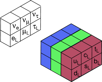
Figure 1: The left-handed doublets of quarks and leptons that inspire the structure of the electroweak theory.

and a few fundamental forces derived from gauge symmetries. The quarks are influenced by the strong interaction, and so carry color, the strong-interaction charge, whereas the leptons do not feel the strong interaction, and are colorless. By pointlike, we understand that the quarks and leptons show no evidence of internal structure at the current limit of our resolution, ($r\mathop{\raisebox{-1.72218pt}{\hbox to0.0pt{$\sim$\hss}}\raisebox{1.72218pt}{$<$}}10^{-18}\hbox{ m}$).

The notion that the quarks and leptons are elementary—structureless and indivisible—is necessarily provisional. Elementarity is one of the aspects of our picture of matter that we test ever more stringently as we improve the resolution with which we can examine the quarks and leptons. For the moment, the world’s most powerful microscope is the Tevatron Collider at Fermilab, where collisions of 980-GeV protons with 980-GeV antiprotons are studied in the CDF and DØ detectors. The most spectacular collision recorded so far, which is to say the closest look humans have ever had at anything, is the CDF two-jet event shown in Figure 2.

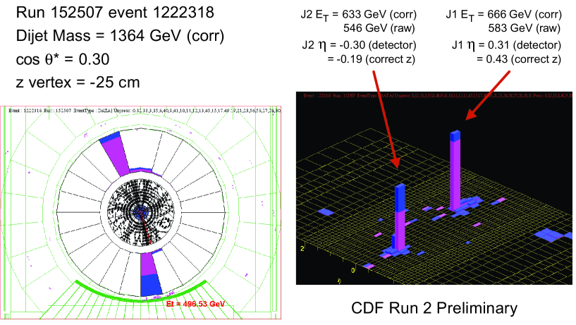
Figure 2: A Tevatron Collider event with $1364\hbox{ GeV}$ of transverse energy, recorded in the CDF detector. The left panel shows an end view of the detector, with tracking chambers at the center and calorimeter segments at medium and large radii. The right panel shows the Lego^TM plot of energy deposited in cells of the cylindrical detector, unrolled. See Ref. [1].

This event almost certainly corresponds to the collision of a quark from the proton with an antiquark from the antiproton. Remarkably, 70% of the energy carried into the collision by proton and antiproton emerges perpendicular to the incident beams. At a given transverse energy $E_{\perp}$, we may roughly estimate the resolution as $r\approx(\hbar c)/E_{\perp}\approx 2\times 10^{-19}\hbox{ TeV}\hbox{ m}/E_{\perp}$.

Looking a little more closely at the constituents of matter, we find that our world is not as neat as the simple cartoon vision of Figure 1. The left-handed and right-handed fermions behave very differently under the influence of the charged-current weak interactions. A more complete picture is given in Figure 3.

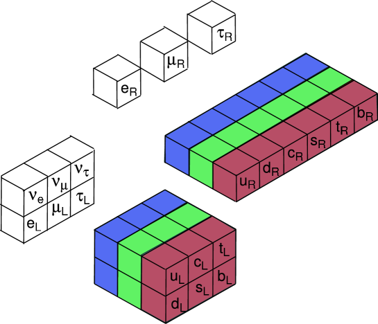
Figure 3: The left-handed doublets and right-handed singlets of quarks and leptons.

This figure represents the way we looked at the world before the discovery of neutrino oscillations that require neutrino mass and almost surely imply the existence of right-handed neutrinos. Neutrinos aside, the striking fact is the asymmetry between left-handed fermion doublets and right-handed fermion singlets, which is manifested in parity violation in the charged-current weak interactions. What does this distinction mean?

All of us in San Miguel Regla have learned about parity violation at school, but it came as a stunning surprise to our scientific ancestors. In 1956, Wu and collaborators [3] studied the $\beta$-decay $\mbox{${}^{60}\mathrm{Co}$}\to\mbox{${}^{60}\mathrm{Ni}$}\;e^{-}\bar{\nu}_{e}$ and observed a correlation between the direction $\hat{p}_{e}$ of the outgoing electron and the spin vector $\vec{J}$ of the polarized ${}^{60}\mathrm{Co}$ nucleus. Spatial reflection, or parity, leaves the (axial vector) spin unchanged, $\mathcal{P}:\vec{J}\to\vec{J}$, but reverses the electron direction, $\mathcal{P}:\hat{p}_{e}\to-\hat{p}_{e}$. Accordingly, the correlation $\vec{J}\cdot\hat{p}_{e}$ is manifestly parity violating. Experiments in the late 1950s established that (charged-current) weak interactions are left-handed, and motivated the construction of a manifestly parity-violating theory of the weak interactions with only a left-handed neutrino $\nu_{\mathrm{L}}$. The left-handed doublets are an important element of the electroweak theory that I will review in Lecture 6

Perhaps our familiarity with parity violation in the weak interactions has dulled our senses a bit. It seems to me that nature’s broken mirror—the distinction between left-handed and right-handed fermions—qualifies as one of the great mysteries. Even if we will not get to the bottom of this mystery next week or next year, it should be prominent in our consciousness—and among the goals we present to others as the aspirations of our science.

There is more to our understanding of the world than Figure 3 reveals. The electroweak gauge symmetry is hidden, $\mathrm{SU(2)}_{\mathrm{L}}\otimes\mathrm{U(1)}_{Y}\rightarrow\mathrm{U(1)_{em}}.$ If it were not, the world would be very different: $\Box$ All the quarks and leptons would be massless and move at the speed of light. $\Box$ Electromagnetism as we know it would not exist, but there would be a long-range hypercharge force. $\Box$ The strong interaction, QCD, would confine quarks and generate baryon masses roughly as we know them. $\Box$ The Bohr radius of “atoms” consisting of an electron or neutrino attracted by the hypercharge interaction to the nucleons would be infinite. $\Box$ Beta decay, inhibited in our world by the great mass of the $W$ boson, would not be weak. $\Box$ The unbroken $\mathrm{SU(2)}_{\mathrm{L}}$ interaction would confine objects that carry weak isospin.

It is fair to say that electroweak symmetry breaking shapes our world! In fact, when we take into account every aspect of the influence of the strong interactions, the analysis of how the world would be is very subtle and fascinating. Please take time to think about

Problem 1

What would the everyday world be like if the $\mathrm{SU(2)}_{\mathrm{L}}\otimes\mathrm{U(1)}_{Y}$ electroweak symmetry were exact? Consider the effects of all of the $\mathrm{SU(3)_{c}}\otimes\mathrm{SU(2)}_{\mathrm{L}}\otimes\mathrm{U(1)}_{Y}$ gauge interactions.

1.3 Toward the double simplex

We have seen that both quarks and leptons are spin-$\cfrac{1}{2}$, pointlike fermions that occur in $\mathrm{SU(2)}_{\mathrm{L}}$ doublets. The obvious difference is that quarks carry $\mathrm{SU(3)_{c}}$ color charge whereas leptons do not, so we could imagine that quarks and leptons are simply distinct and unrelated species. But we have reason to believe otherwise. The proton’s electric charge very closely balances the electron’s, $(Q_{p}+Q_{e})/e<10^{-21}$ [2], suggesting that there must be a link between protons—hence, quarks—and electrons—hence, leptons. Moreover, quarks and leptons are required, in matched pairs, for the electroweak theory to be anomaly-free, so that quantum corrections respect the symmetries on which the theory is based. Before we examine the connection between quarks and leptons, take a moment to consider the implications of ordinary matter that is not exactly neutral:

Problem 2

How large would the imbalance between proton and electron charges need to be for the resulting electrostatic repulsion of un-ionized (nearly neutral) hydrogen atoms to account for the expansion of the Universe? To make your estimate, compare the electrostatic repulsion with the gravitational attraction of two hydrogen atoms. See Ref. [4].

It is fruitful to display the color-triplet red, green, and blue quarks in the equilateral triangle weight diagram for the 3 representation of $\mathrm{SU(3)}_{\mathrm{c}}$, as shown in Figure 4. There I have filled in the plane between them to indicate the transitions mediated by gluons.

Figure 4: A color triplet of quarks and a color singlet lepton, arrayed to explore lepton number as a fourth color.

The equality of proton and (anti)electron charges and the need to cancel anomalies in the electroweak theory suggest that we join the quarks and leptons in an extended family, or multiplet. Pati and Salam [5] provided an apt metaphor when they proposed that we regard lepton number as a fourth color. To explore that possibility, I have placed the lepton in Figure 4 at the apex of a tetrahedron that corresponds to the fundamental 4 representation of $\mathrm{SU(4)}$.

If $\mathrm{SU(4)}$ is not merely a useful classification symmetry for the quarks and leptons, but a gauge symmetry, then there must be new interactions that transform quarks into leptons, as indicated by the gold lines in Figure 5.

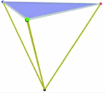
Figure 5: Tetrahedron representing the 4 representation of $\mathrm{SU(4)}$, showing the hypothetical leptoquark transitions.

If leptoquark transitions exist, they can mediate reactions that change baryon and lepton number, such as proton decay. The long proton lifetime [2] tells us that, if leptoquark transitions do exist, they must be far weaker than the strong, weak, and electromagnetic interactions of the standard model. What accounts for the feebleness of leptoquark transitions?

Our world isn’t built of a single quark flavor and a single lepton flavor. The left-handed quark and lepton doublets offer a key clue to the structure of the weak interactions. We can represent the $(u_{\mathrm{L}},d_{\mathrm{L}})$ and $(\nu_{\mathrm{L}},e_{\mathrm{L}})$ doublets by decorating the tetrahedron, as shown in Figure 6.

Figure 6: The $\mathrm{SU(4)}$ tetrahedron, decorated with left-handed fermions.

The orange stalks connecting $u_{\mathrm{L}}\leftrightarrow d_{\mathrm{L}}$ and $\nu_{\mathrm{L}}\leftrightarrow e_{\mathrm{L}}$ represent the $W$-bosons that mediate the charged-current weak interactions.

What about the right-handed fermions? In quantum field theory, it is equivalent to talk about left-handed antifermions. That observation motivates me to display the right-handed quarks and leptons as decorations on an inverted tetrahedron. The right-handed fermions are, by definition, singlets under the usual left-handed weak isospin, $\mathrm{SU(2)}_{\mathrm{L}}$, so I give the decorations a different orientation. We do not know whether the pairs of quarks and leptons carry a right-handed weak isospin, in other words, whether they make up $\mathrm{SU(2)}_{\mathrm{R}}$ doublets. We do know that we have—as yet—no experimental evidence for right-handed charged-current weak interactions. Accordingly, I will generally display the right-handed fermions without a connecting $W_{\mathrm{R}}$-boson, as shown in the left panel of Figure 7.

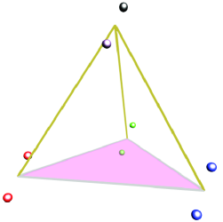
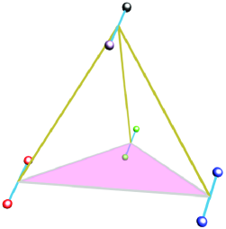
Figure 7: The inverted tetrahedron, decorated with right-handed quark $(d_{\mathrm{R}},u_{\mathrm{R}})$ and lepton $(e_{\mathrm{R}},\nu_{\mathrm{R}})$ pairs. The left panel depicts our current understanding, without right-handed charged currents; the right panel shows how a $W_{\mathrm{R}}$-boson could be added.

Is there a right-handed charged-current interaction? If not, we come back to the question that shook our ancestors: what is the meaning of parity violation, and what does it tell us about the world? If we should discover—or wish to conjecture—a right-handed charged current, it can be added to our graphic, as shown in the right-panel of Figure 7. If there is a right-handed charged-current interaction, restoring parity invariance at high energy scales, what makes that interaction so feeble that we haven’t yet observed it?

Neutrino oscillations make us almost certain that a right-handed neutrino exists, so I have placed a right-handed neutrino in Figure 7. I have given it a different coloration from the established leptons as a reminder that we have not proved its existence, and we do not know its nature.

If parity violation in the weak interactions teaches us of an important asymmetry between left-handed and right-handed fermions, the nonvanishing masses of the quarks and leptons inform us that left and right cannot be entirely separate. Coupling the left-handed particle to its right-handed counterpart is what endows fermions with mass. For example, the mass term of the electron in the Lagrangian of quantum electrodynamics is

$$\mathcal{L}_{e}=-m_{e}\bar{e}e=-m_{e}\bar{e}\left[\cfrac{1}{2}(1-\gamma_{5})+\cfrac{1}{2}(1+\gamma_{5})\right]e=-m_{e}(\bar{e}_{\mathrm{R}}e_{\mathrm{L}}+\bar{e}_{\mathrm{L}}e_{\mathrm{R}})\;.$$ (1.3)

How shall we combine left with right? A suggestive structure is the pair of interpenetrating tetrahedra shown in Figure 8.

    

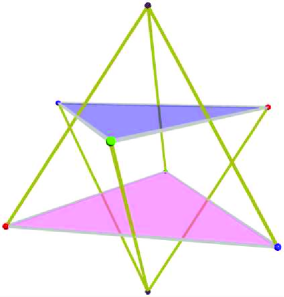
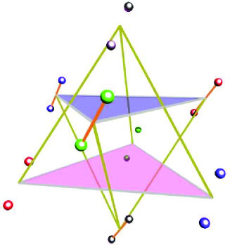
Figure 8: The double simplex, undecorated (left panel) and decorated with one generation of quarks and leptons (right panel).

Mathematicians refer to a tetrahedron as a simplex in three-dimensional space, so I call this construction the double simplex.

The structure of the double simplex is based on the $\mathrm{{SU(4)}\otimes{SU(2)}\otimes{SU(2)}}$ decomposition of $\mathrm{SO(10)}$. A three-dimensional solid (tetrahedron) represents the fundamental 4 representation of $\mathrm{SU(4)}$. It is decorated at the vertices with dumbbells representing the $\mathrm{SU(2)_{L}}$ and $\mathrm{SU(2)_{R}}$ quantum numbers. The vertical coordinate of $\mathrm{SU(4)}$ can be read as $B-L$, the difference of baryon number and lepton number. The group $\mathrm{SO(10)}$ is a useful classification symmetry, because its 16-dimensional fundamental representation contains an entire generation of the known quarks and leptons. Using $\mathrm{SO(10)}$ as a coordinate system, if you like, carries no implication that it is the symmetry of the world, or that it is the basis of a unified theory of the strong, weak, and electromagnetic interactions. The idea of the double simplex is to represent what we know is true, what we hope might be true, and what we don’t know—in other terms, to show the connections that are firmly established, those we believe must be there, and the open issues.

Fermion masses tell us that the left-handed and right-handed fermions are linked, but we do not know what agent makes the connection. In the standard $\mathrm{SU(2)}_{\mathrm{L}}\otimes\mathrm{U(1)}_{Y}$ electroweak theory, it is the Higgs boson—the avatar of electroweak symmetry breaking—that endows the fermions with mass. But this has not been proved by experiment, and it is certainly conceivable that some entirely different mechanism is the source of fermion mass.

I draw the connection between the left-handed and right-handed electrons in Figure 9.

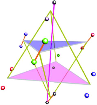
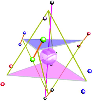
Figure 9: The connection between $e_{\mathrm{R}}$ and $e_{\mathrm{L}}$ implied by the electron’s nonzero mass.

The left-hand panel shows the link between $e_{\mathrm{L}}$ and $e_{\mathrm{R}}$. In the right-hand panel, I show the connection veiled within an opalescent globe that represents our ignorance of the symmetry-hiding phase transition that links left and right. It is excellent to find that the central mystery of the standard model—the nature of electroweak symmetry breaking—appears at the center of the double simplex!

Connecting all the left-handed fermions to their right-handed counterparts leads us to the representation given in Figure 10.

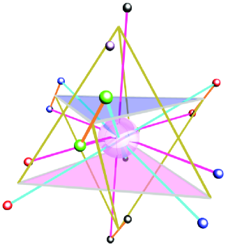
Figure 10: The connections that give rise to mass for the quarks and leptons of the first generation.

Does one agent give masses to all the quarks and leptons? (That is the standard-model solution.) If so, what distinguishes one fermion species from another? We do not know the answer, and for that reason I contend that fermion mass is evidence for physics beyond the standard model. Let us illustrate the point in the standard-model context. The mass of fermion $f$ is given by

$$\mathcal{L}_{f}=-\displaystyle{\frac{{}{\zeta_{f}}v}{\sqrt{2}}}(\bar{f}_{\mathrm{R}}f_{\mathrm{L}}+\bar{f}_{\mathrm{L}}f_{\mathrm{R}})=-\displaystyle{\frac{{}{\zeta_{f}}v}{\sqrt{2}}}\bar{f}f\;,$$ (1.4)

where $v/\sqrt{2}=(G_{\mathrm{F}}\sqrt{8})^{-1/2}\approx 174\hbox{ GeV}$ is the vacuum expectation value of the Higgs field. The Yukawa coupling $\zeta_{f}$ is not predicted by the electroweak theory, nor does the standard model relate different Yukawa couplings. In any event, we do not know whether one agent, or two, or three, will give rise to the electron, up-quark, and down-quark masses.

Of course, the world we have discovered until now consists not only of one family of quarks and one family of leptons, but of the three pairs of quarks and three pairs of leptons enumerated in (1.1) and (1.2). We do not know the meaning of the replicated generations, and indeed we have no experimental indication to tell us which pair of quarks is to be associated with which pair of leptons.

In the absence of any understanding of the relation of one generation to another, I depict the three generations in the double simplex simply by replicating the decorations to include three pairs of quarks and three pairs of leptons, as shown in the left panel of Figure 11.

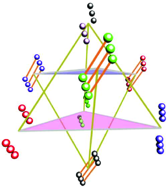
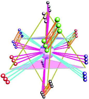
Figure 11: Left panel: Three generations of quarks and leptons. Right panel: The connections that give rise to mass and mixing for three generations of quarks and leptons.

The connections that generate the fermion masses are indicated in the right panel of Figure 11. The Yukawa couplings of the charged leptons and quarks range from $\zeta_{e}\approx 3\times 10^{-6}$ for the electron to $\zeta_{t}\approx 1$ for the top quark. In the case of more than one generation, the connections that endow the fermions with mass also determine the mixing among generations, the suppressed transitions such as $u\leftrightarrow s$ and $u\leftrightarrow b$. With three generations, the Yukawa couplings may have complex phases that give rise to $\mathcal{CP}$-violating transitions. Although it is correct to say that the standard model describes the observed examples of $\mathcal{CP}$ violation, I would like to insist that because the standard model does not prescribe the Yukawa couplings, $\mathcal{CP}$ violation—like fermion mass—is evidence for physics beyond the standard model.

Let us return to the point that the charge conjugate of a left-handed field is right-handed. If the field $\psi$ annihilates a particle, then its charge-conjugate filed $\psi^{\mathrm{c}}\equiv\mathcal{C}\bar{\psi}^{\mathrm{T}}$ annihilates the corresponding antiparticle. In terms of Dirac matrices, the charge-conjugation operator is

$$\mathcal{C}=i\gamma^{2}\gamma^{0}=-\mathcal{C}^{-1}=-\mathcal{C}^{\dagger}=-\mathcal{C}^{\mathrm{T}}\;.$$ (1.5)

The left-handed component of the charge-conjugate field is

$${\psi^{\mathrm{c}}_{\mathrm{L}}} = \cfrac{1}{2}(1-\gamma_{5})\psi^{\mathrm{c}}=\cfrac{1}{2}(1-\gamma_{5})\mathcal{C}\bar{\psi}^{\mathrm{T}}$$

$$= \mathcal{C}\cfrac{1}{2}(1-\gamma_{5})\bar{\psi}^{\mathrm{T}}=\mathcal{C}[\bar{\psi}\cfrac{1}{2}(1-\gamma_{5})]^{\mathrm{T}}$$

$$= \mathcal{C}(\bar{\psi}_{\mathrm{R}})^{\mathrm{T}}={(\psi_{\mathrm{R}})^{\mathrm{c}}}\;,$$

which is indeed the charge conjugate of the right-handed component of the Dirac field $\psi$.

With this connection in mind, we can now think of the double simplex as composed of left-handed particles and left-handed antiparticles. When we combine the two sets of particles into one representation, we are invited to consider the possibility of new transformations that take any member of the extended family into any other. The agents of change will be new gauge bosons, since gauge-boson interactions preserve chirality. I connect the hitherto unconnect vertices of the (undecorated) double simplex in Figure 12.

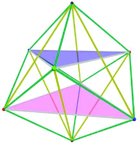
Figure 12: The double simplex, with additional interactions suggested by the shape of the figure indicated as green links.

The hypothetical new interactions are easy to visualize, because the double simplex can be inscribed in a cube. Do some of these interactions exist? If so, why are they so weak that we have not yet observed them?

The object of our double-simplex construction project has been to identify important topical questions for particle physics without plunging into formalism. As a theoretical physicist, I have deep respect for the power of mathematics to serve as a refiner’s fire for our ideas. But I hope this exercise has helped you to see the power and scope of physical reasoning and the insights that can come from building and looking at a physical object with an inquiring spirit—even if the physical object inhabits an abstract space!

In the spirit of providing homework for life, here are some of the questions we have encountered in this first lecture:

First Harvest of Questions

• Are quarks and leptons elementary?

• What is the relationship of quarks to leptons?

• Are there right-handed weak interactions?

• Are there new quarks and leptons?

• Are there new gauge interactions linking quarks and leptons?

• What is the relationship of left-handed & right-handed particles?

• What is the nature of the right-handed neutrino?

• What is the nature of the mysterious new force that hides electroweak symmetry?

• Are there different kinds of matter?

• Are there new forces of a novel kind?

• What do generations mean? Is there a family symmetry?

• What makes a top quark a top quark, and an electron an electron?

• What is the (grand) unifying symmetry?

2 The Electroweak Theory

To provide us with a common starting point for our investigation of theories that extend the standard model, we devote this lecture to a survey of the electroweak theory. As I have emphasized elsewhere [6], the theory of the strong interactions, quantum chromodynamics, is an essential element of the standard model, but it is by contemplating the electroweak theory that we are led most quickly to see the shortcomings of the standard model.

We shall begin by recalling the idea of gauge theories, and then use the strategy we uncover there to construct the electroweak theory. Applying the theory to quarks, we come upon the need to inhibit flavor-changing neutral currents that motivated the introduction of the charmed quark. Then we swiftly review the tests of the electroweak theory that have led us, over the past decade, to elevate it to the status of a (provisional!) law of nature. A profound puzzle raised by the electroweak theory, as we shall see, is why empty space—the vacuum—is so nearly massless. We will recall bounds on the mass of the Higgs boson and then conclude our little tour by looking at the electroweak scale and beyond.

2.1 How Symmetries Lead to Interactions

Suppose that we knew the Schrödinger equation, but not the laws of electrodynamics. Would it be possible to derive—in other words, to guess—Maxwell’s equations from a gauge principle. The answer is yes! it is worthwhile to trace the steps in the argument in detail.

A quantum-mechanical state is described by a complex Schrödinger wave function $\psi(x)$. Quantum-mechanical observables involve inner products of the form

$$\langle\mathcal{O}\rangle=\int d^{n}\!x\>\psi^{*}{\mathcal{O}}\psi,$$ (2.1)

which are unchanged under a global phase rotation:

$$\psi(x)\rightarrow e^{i\theta}\psi(x)\qquad\psi^{*}(x)\rightarrow e^{-i\theta}\psi^{*}(x).$$ (2.2)

In other words, the absolute phase of the wave function cannot be measured and is a matter of convention. Relative phases between wave functions, as measured in interference experiments, are unaffected by such a global rotation.

This raises the question: Are we free to choose one phase convention in San Miguel Regla and another in Geneva? Differently stated, can quantum mechanics be formulated to be invariant under local (position-dependent) phase rotations

$$\psi(x)\rightarrow\psi^{\prime}(x)=e^{i\alpha(x)}\psi(x)\;?$$ (2.3)

We shall see that this can be accomplished, but at the price of introducing an interaction that we will construct to be electromagnetism.

The quantum-mechanical equations of motion, such as the Schrödinger equation, always involve derivatives of the wave function $\psi$, as do many observables. Under local phase rotations, these transform as

$$\partial_{\mu}\psi(x)\rightarrow\partial_{\mu}\psi^{\prime}=e^{i\alpha(x)}[\partial_{\mu}\psi(x)+i(\partial_{\mu}\alpha(x))\psi(x)],$$ (2.4)

which involves more than a mere phase change. The additional gradient-of-phase term spoils local phase invariance. Local phase invariance may be achieved, however, if the equations of motion and the observables involving derivatives are modified by the introduction of the electromagnetic field $A_{\mu}(x)$. If the gradient $\partial_{\mu}$ is everwhere replaced by the gauge-covariant derivative

$$\mathcal{D}_{\mu}\equiv\partial_{\mu}+ieA_{\mu},$$ (2.5)

where $e$ is the charge in natural units of the particle described by $\psi(x)$ and the field $A_{\mu}(x)$ transforms under phase rotations (2.3) as

$$A_{\mu}(x)\rightarrow A_{\mu}^{\prime}(x)\equiv A_{\mu}(x)-(1/e)\partial_{\mu}\alpha(x),$$ (2.6)

it is easily verified that under local phase transformations

$$\mathcal{D}_{\mu}\psi(x)\rightarrow e^{i\alpha(x)}\mathcal{D}_{\mu}\psi(x).$$ (2.7)

Consequently quantities such as $\psi^{*}\mathcal{D}_{\mu}\psi$ are invariant under local phase transformations. The required transformation law (2.6) for the four-vector potential $A_{\mu}$ is precisely the form of a gauge transformation in electrodynamics. Moreover, the covariant derivative defined in (2.5) corresponds to the familiar replacement $p\rightarrow p-eA$. Thus the form of the coupling $(\mathcal{D}_{\mu}\psi)$ between the electromagnetic field and matter is suggested, if not uniquely dictated, by local phase invariance.

A photon mass term would have the form

$$\mathcal{L}_{\gamma}={\scriptstyle\frac{1}{2}}m^{2}A^{\mu}A_{\mu},$$ (2.8)

which obviously violates local gauge invariance because

$$A^{\mu}A_{\mu}\rightarrow(A^{\mu}-\partial^{\mu}\alpha)(A_{\mu}-\partial_{\mu}\alpha)\neq A^{\mu}A_{\mu}.$$ (2.9)

Thus we find that local gauge invariance has led us to the existence of a massless photon.

This example has shown the possibility of using local gauge invariance as a dynamical principle. We have derived the content of Maxwell’s equations from a symmetry principle. We can think of quantum electrodynamics as the gauge theory based on $\mathrm{U(1)}$ phase symmetry.

We can abstract from this discussion a general procedure. First, recognize a symmetry of Nature, perhaps by observing a conservation law, and build it into the laws of physics. Then impose the symmetry in a stricter local form. By a generalization of the arithmetic we have just recited, the local gauge symmetry leads to new interactions, mediated by massless vector fields, the gauge bosons. As we have seen, the interaction of the gauge fields with matter is given by “minimal coupling” to the conserved current that corresponds to the symmetry. If the symmetry is non-Abelian, imposing the symmetry also leads to interactions among the gauge bosons, since they carry the conserved charge.

Posed as a problem in mathematics, construction of a gauge theory is always possible, at the level of a classical Lagrangian. Formulating a consistent quantum theory may require additional vigilance. The formalism offers no guarantee that the gauge symmetry was chosen wisely; that verdict is left to experiment!

2.2 Hiding a Gauge Symmetry

The gauge-theory paradigm is constraining and it is predictive, but there is an obstacle to surmount if we want to apply it to all the interactions. As we have just seen, local gauge invariance is incompatible with a massive gauge boson. Yet we have known since the 1930s that the (charged-current) weak interaction has a very short range, on the order of $10^{-15}\hbox{ cm}$, so must be mediated by a massive $\mathcal{O}(100\hbox{ GeV})$ force carrier. Happily, condensed-matter physics provides us with an example of a physical system in which the photon of QED acquires a mass inside a medium, as a consequence of a symmetry-reducing phase transition: superconductivity.

Superconducting materials display two kinds of miraculous behavior: they carry an electric current without resistance, and they expel magnetic fields. In the Ginzburg-Landau description [7] of the superconducting phase transition, a superconducting material is regarded as a collection of two kinds of charge carriers: normal, resistive carriers, and superconducting, resistanceless carriers.

In the absence of a magnetic field, the free energy of the superconductor is related to the free energy in the normal state through

$$G_{\rm super}(0)=G_{\rm normal}(0)+\alpha\left|\psi\right|^{2}+\beta\left|\psi\right|^{4}\;\;,$$ (2.10)

where $\alpha$ and $\beta$ are phenomenological parameters and $\left|\psi\right|^{2}$ is an order parameter that measures the density of superconducting charge carriers. The parameter $\beta$ is non-negative, so that the free energy is bounded from below.

Above the critical temperature for the onset of superconductivity, the parameter $\alpha$ is positive and the free energy of the substance is supposed to be an increasing function of the density of superconducting carriers, as shown in Figure 13(a). The state of minimum energy, the vacuum state, then corresponds to a purely resistive flow, with no superconducting carriers active. Below the critical temperature, the parameter $\alpha$ becomes negative and the free energy is minimized when $\langle|\psi|^{2}\rangle_{0}=\psi^{2}_{0}\neq 0$, as illustrated in Figure 13(b).

Figure 13: Ginzburg-Landau description of the superconducting phase transition.

This is a nice cartoon description of the superconducting phase transition, but there is more. In an applied magnetic field $\vec{H}$, the free energy is

$$G_{\rm super}(\vec{H})=G_{\rm super}(0)+\frac{\vec{H}^{2}}{8\pi}+\frac{1}{2m^{\star}}|-i\hbar\nabla\psi-(e^{\star}/c)\vec{A}\psi|^{2}\;\;,$$ (2.11)

where $e^{\star}$ and $m^{\star}$ are the charge ($-2$ units) and effective mass of the superconducting carriers. In a weak, slowly varying field $\vec{H}\approx 0$, when we can approximate $\psi\approx\psi_{0}$ and $\nabla\psi\approx 0$, the usual variational analysis leads to the equation of motion,

$$\nabla^{2}\vec{A}-\frac{4\pi e^{\star}}{m^{\star}c^{2}}\left|\psi_{0}\right|^{2}\vec{A}=0\;\;,$$ (2.12)

the wave equation of a massive photon. In other words, the photon acquires a mass within the superconductor. This is the origin of the Meissner effect, the exclusion of a magnetic field from a superconductor. More to the point for our purposes, it shows how a symmetry-hiding phase transition can lead to a massive gauge boson.

2.3 Constructing the Electroweak Theory

Let us review the essential elements of the $\mathrm{SU(2)}_{\mathrm{L}}\otimes\mathrm{U(1)}_{Y}$ electroweak theory [8]. The electroweak theory takes three crucial clues from experiment:

• The existence of left-handed weak-isospin doublets,

  $$\left(\begin{array}[]{c}\nu_{e}\\ e\end{array}\right)_{\mathrm{L}}\qquad\left(\begin{array}[]{c}\nu_{\mu}\\ \mu\end{array}\right)_{\mathrm{L}}\qquad\left(\begin{array}[]{c}\nu_{\tau}\\ \tau\end{array}\right)_{\mathrm{L}}$$

  and

  $$\left(\begin{array}[]{c}u\\ d^{\prime}\end{array}\right)_{\mathrm{L}}\qquad\left(\begin{array}[]{c}c\\ s^{\prime}\end{array}\right)_{\mathrm{L}}\qquad\left(\begin{array}[]{c}t\\ b^{\prime}\end{array}\right)_{\mathrm{L}}\;;$$

• The universal strength of the weak interactions;

• The idealization that neutrinos are massless.

To save writing, we shall construct the electroweak theory as it applies to a single generation of leptons. In this form, it is neither complete nor consistent: anomaly cancellation requires that a doublet of color-triplet quarks accompany each doublet of color-singlet leptons. However, the needed generalizations are simple enough to make that we need not write them out.

To incorporate electromagnetism into a theory of the weak interactions, we add to the $\mathrm{SU(2)_{L}}$ family symmetry suggested by the first two experimental clues a $\mathrm{U(1)}_{Y}$ weak-hypercharge phase symmetry. We begin by specifying the fermions: a left-handed weak isospin doublet

$${{\sf L}}=\left(\begin{array}[]{c}\nu_{e}\\ e\end{array}\right)_{\mathrm{L}}$$ (2.13)

with weak hypercharge $Y_{\mathrm{L}}=-1$, and a right-handed weak isospin singlet

$${{\sf R}}\equiv e_{\mathrm{R}}$$ (2.14)

with weak hypercharge $Y_{\mathrm{R}}=-2$.

The electroweak gauge group, $\mathrm{SU(2)}_{\mathrm{L}}\otimes\mathrm{U(1)}_{Y}$, implies two sets of gauge fields: a weak isovector $\vec{b}_{\mu}$, with coupling constant $g$, and a weak isoscalar ${{\mathcal{A}}}_{\mu}$, with coupling constant $g^{\prime}$. Corresponding to these gauge fields are the field-strength tensors

$$F^{\ell}_{\mu\nu}=\partial_{\nu}b^{\ell}_{\mu}-\partial_{\mu}b^{\ell}_{\nu}+g\varepsilon_{jk\ell}b^{j}_{\mu}b^{k}_{\nu}\;,$$ (2.15)

for the weak-isospin symmetry, and

$$f_{\mu\nu}=\partial_{\nu}{{\mathcal{A}}}_{\mu}-\partial_{\mu}{{\mathcal{A}}}_{\nu}\;,$$ (2.16)

for the weak-hypercharge symmetry. We may summarize the interactions by the Lagrangian

$$\mathcal{L}=\mathcal{L}_{\rm gauge}+\mathcal{L}_{\rm leptons}\ ,$$ (2.17)

with

$$\mathcal{L}_{\rm gauge}=-\cfrac{1}{4}F_{\mu\nu}^{\ell}F^{\ell\mu\nu}-\cfrac{1}{4}f_{\mu\nu}f^{\mu\nu},$$ (2.18)

and

$$\mathcal{L}_{\rm leptons} = \overline{{\sf R}}\>i\gamma^{\mu}\!\left(\partial_{\mu}+i\frac{g^{\prime}}{2}{\cal A}_{\mu}Y\right)\!{\sf R}$$

$$+ \overline{{\sf L}}\>i\gamma^{\mu}\!\left(\partial_{\mu}+i\frac{g^{\prime}}{2}{\cal A}_{\mu}Y+i\frac{g}{2}\vec{\tau}\cdot\vec{b}_{\mu}\right)\!{\sf L}.$$

The $\mathrm{SU(2)}_{\mathrm{L}}\otimes\mathrm{U(1)}_{Y}$ gauge symmetry forbids a mass term for the electron in the matter piece (2.3). Moreover, the theory we have described contains four massless electroweak gauge bosons, namely ${{\mathcal{A}}}_{\mu}$, $b^{1}_{\mu}$, $b^{2}_{\mu}$, and $b^{3}_{\mu}$, whereas Nature has but one: the photon. To give masses to the gauge bosons and constituent fermions, we must hide the electroweak symmetry.

To endow the intermediate bosons of the weak interaction with mass, we take advantage of a relativistic generalization of the Ginzburg-Landau phase transition known as the Higgs mechanism [9]. We introduce a complex doublet of scalar fields

$$\phi\equiv\left(\begin{array}[]{c}\phi^{+}\\ \phi^{0}\end{array}\right)$$ (2.20)

with weak hypercharge $Y_{\phi}=+1$. Next, we add to the Lagrangian new (gauge-invariant) terms for the interaction and propagation of the scalars,

$$\mathcal{L}_{\rm scalar}=(\mathcal{D}^{\mu}\phi)^{\dagger}(\mathcal{D}_{\mu}\phi)-V(\phi^{\dagger}\phi),$$ (2.21)

where the gauge-covariant derivative is

$$\mathcal{D}_{\mu}=\partial_{\mu}+i\frac{g^{\prime}}{2}{\cal A}_{\mu}Y+i\frac{g}{2}\vec{\tau}\cdot\vec{b}_{\mu}\;,$$ (2.22)

and the potential interaction has the form

$$V(\phi^{\dagger}\phi)=\mu^{2}(\phi^{\dagger}\phi)+\left|\lambda\right|(\phi^{\dagger}\phi)^{2}.$$ (2.23)

We are also free to add a Yukawa interaction between the scalar fields and the leptons,

$$\mathcal{L}_{\rm Yukawa}=-\zeta_{e}\left[\overline{{\sf R}}(\phi^{\dagger}{\sf L})+(\overline{{\sf L}}\phi){\sf R}\right].$$ (2.24)

We then arrange the scalar self-interactions so that the vacuum state corresponds to a broken-symmetry solution. The electroweak symmetry is spontaneously broken if the parameter $\mu^{2}<0$. The minimum energy, or vacuum state, may then be chosen to correspond to the vacuum expectation value

$$\langle\phi\rangle_{0}=\left(\begin{array}[]{c}0\\ v/\sqrt{2}\end{array}\right)\;,$$ (2.25)

where $v=\sqrt{-\mu^{2}/\left|\lambda\right|}$. Let us verify that the vacuum (2.25) indeed breaks the gauge symmetry. The vacuum state $\langle\phi\rangle_{0}$ is invariant under a symmetry operation $\exp{(i\alpha{\mathcal{G}})}$ corresponding to the generator ${\mathcal{G}}$ provided that $\exp{(i\alpha{\mathcal{G}})}\langle\phi\rangle_{0}=\langle\phi\rangle_{0}$, i.e., if ${\mathcal{G}}\langle\phi\rangle_{0}=0$. We easily compute that

$$\tau_{1}\langle\phi\rangle_{0} =\left(\begin{array}[]{cc}0&1\\ 1&0\end{array}\right)\left(\begin{array}[]{c}0\\ v/\sqrt{2}\end{array}\right) =\left(\begin{array}[]{c}v/\sqrt{2}\\ 0\end{array}\right)\neq 0\quad\hbox{broken!}$$ (2.32)

$$\tau_{2}\langle\phi\rangle_{0} =\left(\begin{array}[]{cc}0&-i\\ i&0\end{array}\right)\left(\begin{array}[]{c}0\\ v/\sqrt{2}\end{array}\right) =\left(\begin{array}[]{c}-iv/\sqrt{2}\\ 0\end{array}\right)\neq 0\quad\hbox{broken!}$$ (2.39)

$$\tau_{3}\langle\phi\rangle_{0} =\left(\begin{array}[]{cc}1&0\\ 0&-1\end{array}\right)\left(\begin{array}[]{c}0\\ v/\sqrt{2}\end{array}\right) =\left(\begin{array}[]{c}0\\ -v/\sqrt{2}\end{array}\right)\neq 0\quad\hbox{broken!}$$ (2.46)

$$Y\langle\phi\rangle_{0} =Y_{\phi}\langle\phi\rangle_{0}=+1\langle\phi\rangle_{0}= \left(\begin{array}[]{c}0\\ v/\sqrt{2}\end{array}\right)\neq 0\quad\hbox{broken!}$$ (2.49)

However, if we examine the effect of the electric charge operator $Q$ on the (electrically neutral) vacuum state, we find that

$$Q\langle\phi\rangle_{0} =\cfrac{1}{2}(\tau_{3}+Y)\langle\phi\rangle_{0}\qquad\quad =\cfrac{1}{2}\left(\begin{array}[]{cc}Y_{\phi}+1&0\\ 0&Y_{\phi}-1\end{array}\right)\langle\phi\rangle_{0}$$ (2.52)

$$=\left(\begin{array}[]{cc}1&0\\ 0&0\end{array}\right)\left(\begin{array}[]{c}0\\ v/\sqrt{2}\end{array}\right) =\left(\begin{array}[]{c}0\\ 0\end{array}\right)\quad\hbox{{unbroken!}}$$ (2.59)

The original four generators are all broken, but electric charge is not. It appears that we have accomplished our goal of breaking $\mathrm{SU(2)_{L}}\otimes\mathrm{U(1)}_{Y}\to\mathrm{U(1)}_{\mathrm{em}}$. We expect the photon to remain massless, and expect the gauge bosons that correspond to the generators $\tau_{1}$, $\tau_{2}$, and $\kappa\equiv\cfrac{1}{2}(\tau_{3}-Y)$ to acquire masses.

To establish the particle content of the theory, we expand about the vacuum state, letting

$$\phi=\displaystyle{\left(\begin{array}[]{c}0\\ (v+\eta)/\sqrt{2}\end{array}\right)}$$ (2.60)

in unitary gauge. The Lagrangian for the scalars becomes

$$\mathcal{L}_{\mathrm{scalar}} = \cfrac{1}{2}(\partial^{\mu}\eta)(\partial_{\mu}\eta)-\mu^{2}\eta^{2}$$

$$+\frac{v^{2}}{8}[g^{2}\left|b_{1}-ib_{2}\right|^{2}+(g^{\prime}\mathcal{A}_{\mu}-gb_{\mu}^{3})^{2}]$$

$$+\mbox{ interaction terms}.$$

The Higgs boson $\eta$ has acquired a $(\mbox{mass})^{2}$ $M_{H}^{2}=-2\mu^{2}>0$. Now let us expand the terms proportional to $v^{2}/8$. Identifying $W^{\pm}=\cfrac{1}{\sqrt{2}}(b_{1}\mp ib_{2})$, we find

$$\frac{g^{2}v^{2}}{8}(\left|W^{+}_{\mu}\right|^{2}+\left|W^{-}_{\mu}\right|^{2})\;,$$ (2.62)

which implies $M_{W^{\pm}}=gv/2$. Next, we define the orthogonal combinations

$$Z_{\mu}=\frac{-g^{\prime}\mathcal{A}_{\mu}+gb_{\mu}^{3}}{\sqrt{g^{2}+g^{\prime 2}}}\;,\quad\quad\qquad A_{\mu}=\frac{g\mathcal{A}_{\mu}+g^{\prime}b_{\mu}^{3}}{\sqrt{g^{2}+g^{\prime 2}}}\;,$$ (2.63)

and conclude that $M_{Z^{0}}=\sqrt{g^{2}+g^{\prime 2}}\;v/2=M_{W}\sqrt{1+g^{\prime 2}/g^{2}}$ and $M_{A}=0$. In the broken-symmetry situation, the Yukawa term becomes

$$\mathcal{L}_{\mathrm{Yukawa}} = -\zeta_{e}\frac{(v+\eta)}{\sqrt{2}}(\bar{e}_{\mathsf{R}}e_{\mathsf{L}}+\bar{e}_{\mathsf{L}}e_{\mathsf{R}})$$ (2.64)

$$= -\frac{\zeta_{e}v}{\sqrt{2}}\bar{e}e-\frac{\zeta_{e}\eta}{\sqrt{2}}\bar{e}e\;,$$

so that the electron acquires a mass $m_{e}=\zeta_{e}v/\sqrt{2}$ and the Higgs-boson coupling to electrons is $m_{e}/v\propto\hbox{fermion mass}$.

Let us summarize. As a result of spontaneous symmetry breaking, the weak bosons acquire masses, as auxiliary scalars assume the role of the third (longitudinal) degrees of freedom of what had been massless gauge bosons. Specifically, the mediator of the charged-current weak interaction, $W^{\pm}=(b_{1}\mp ib_{2})/\sqrt{2}$, acquires a mass characterized by $M_{W}^{2}=\pi\alpha/G_{\mathrm{F}}\sqrt{2}\sin^{2}{\theta_{W}}$, where $\sin^{2}\theta_{W}=g^{\prime 2}/(g^{2}+g^{\prime 2})$ is the weak mixing parameter. The mediator of the neutral-current weak interaction, $Z=b_{3}\cos{\theta_{W}}-\mathcal{A}\sin{\theta_{W}}$, acquires a mass characterized by $M_{Z}^{2}=M_{W}^{2}/\cos^{2}{\theta_{W}}$. After spontaneous symmetry breaking, there remains an unbroken $\mathrm{U(1)}_{\mathrm{em}}$ phase symmetry, so that electromagnetism is mediated by a massless photon, $A=\mathcal{A}\cos{\theta_{W}}+b_{3}\sin{\theta_{W}}$, coupled to the electric charge $e=gg^{\prime}/\sqrt{g^{2}+g^{\prime 2}}$. As a vestige of the spontaneous breaking of the symmetry, there remains a massive, spin-zero particle, the Higgs boson. The mass of the Higgs scalar is given symbolically as $M_{H}^{2}=-2\mu^{2}>0$, but we have no prediction for its value. Though what we take to be the work of the Higgs boson is all around us, the Higgs particle itself has not yet been observed. The fermions (the electron in our abbreviated treatment) acquire masses as well; these are determined not only by the scale of electroweak symmetry breaking, $v$, but also by their Yukawa interactions with the scalars.

To determine the values of the coupling constants and the electroweak scale—hence the masses of $W^{\pm}$ and $Z^{0}$—we now examine the interactions terms we wrote symbolically in (2.3).

2.3.1 Charged-current interactions

The interactions of the $W$-boson with the leptons are given by

$$\mathcal{L}_{W\mathrm{-lep}}=\frac{-g}{2\sqrt{2}}\left[\bar{\nu}_{e}\gamma^{\mu}(1-\gamma_{5})eW^{+}_{\mu}+\bar{e}\gamma^{\mu}(1-\gamma_{5})\nu_{e}W^{-}_{\mu}\right],\mathrm{etc.},$$ (2.65)

so the Feynman rule for the $\nu_{e}eW$ vertex is

The $W$-boson propagator (in unitary gauge) is   

Let us compute the cross section for inverse muon decay in the electroweak theory. We find

$$\sigma(\nu_{\mu}e\to\mu\nu_{e})=\frac{g^{4}m_{e}E_{\nu}}{16\pi M_{W}^{4}}\;\frac{\left[1-(m_{\mu}^{2}-m_{e}^{2})/2m_{e}E_{\nu}\right]^{2}}{(1+2m_{e}E_{\nu}/M_{W}^{2})}\;,$$ (2.66)

which coincides with the familiar four-fermion result at low energies, provided we identify

$$\frac{g^{4}}{16M_{W}^{2}}=2G_{\mathrm{F}}^{2}\;,$$ (2.67)

(where $G_{\mathrm{F}}=1.16639\times 10^{-5}\hbox{ GeV}^{-2}$ is the Fermi constant) which implies that

$$\frac{g}{2\sqrt{2}}=\left(\frac{G_{\mathrm{F}}M_{W}^{2}}{\sqrt{2}}\right)^{\cfrac{1}{2}}\;.$$ (2.68)

With the aid of our result for the $W$-boson mass, $M_{W^{\pm}}=gv/2$, we determine the electroweak scale,

$$v=\left(G_{\mathrm{F}}\sqrt{2}\right)^{-\cfrac{1}{2}}\approx 246\hbox{ GeV}\;,$$ (2.69)

which implies that $\langle\phi^{0}\rangle_{0}=(G_{\mathrm{F}}\sqrt{8})^{-\cfrac{1}{2}}\approx 174\hbox{ GeV}$.

Let us now investigate the properties of the $W$-boson in terms of its mass, $M_{W}$. Consider first the leptonic disintegration of the $W^{-}$, with decay kinematics specified thus:

The Feynman amplitude for the decay is

$$\mathcal{M}=-i\left(\frac{G_{\mathrm{F}}M_{W}^{2}}{\sqrt{2}}\right)^{\cfrac{1}{2}}\bar{u}(e,p)\gamma_{\mu}(1-\gamma_{5})v(\nu,q)\,\varepsilon^{\mu}\;,$$ (2.70)

where $\varepsilon^{\mu}=(0;\hat{\varepsilon})$ is the polarization vector of the $W$-boson in its rest frame. The square of the amplitude is

$$\left|\mathcal{M}\right|^{2} = \frac{G_{\mathrm{F}}M_{W}^{2}}{\sqrt{2}}\mathrm{tr}\left[\hbox to0.0pt{\hbox to5.00002pt{\hfil$\varepsilon$\hfil}\hss}\hbox{\sl/}(1-\gamma_{5})\hbox to0.0pt{\hbox to5.00002pt{\hfil$q$\hfil}\hss}\hbox{\sl/}(1+\gamma_{5})\hbox to0.0pt{\hbox to5.00002pt{\hfil$\varepsilon$\hfil}\hss}\hbox{\sl/}^{*}p\hbox to0.0pt{\hss\sl/}\right]$$

$$= \displaystyle{\frac{8G_{\mathrm{F}}M_{W}^{2}}{\sqrt{2}}}\left[\varepsilon\cdot q\>\varepsilon^{*}\cdot p-\varepsilon\cdot\varepsilon^{*}\>q\cdot p+\varepsilon\cdot p\>\varepsilon^{*}\cdot q+i\epsilon_{\mu\nu\rho\sigma}\varepsilon^{\mu}q^{\nu}\varepsilon^{*\rho}p^{\sigma}\right]\;.$$

The decay rate is independent of the $W$ polarization, so let us look first at the case of longitudinal polarization $\varepsilon^{\mu}=(0;0,0,1)=\varepsilon^{*\mu}$, to eliminate the last term. For this case, we find

$$\left|\mathcal{M}\right|^{2}=\frac{4G_{\mathrm{F}}M_{W}^{4}}{\sqrt{2}}\sin^{2}\theta\;,$$ (2.72)

so the differential decay rate is

$$\frac{d\Gamma_{0}}{d\Omega}=\frac{\left|\mathcal{M}\right|^{2}}{64\pi^{2}}\>\frac{{\mathcal{S}}_{12}}{M_{W}^{3}}\;,$$ (2.73)

where ${\mathcal{S}}_{12}=\sqrt{[M_{W}^{2}-(m_{e}+m_{\nu})^{2}][M_{W}^{2}-(m_{e}-m_{\nu})^{2}]}=M_{W}^{2}$, so that

$$\frac{d\Gamma_{0}}{d\Omega}=\frac{G_{\mathrm{F}}M_{W}^{3}}{16\pi^{2}\sqrt{2}}\sin^{2}\theta\;,$$ (2.74)

and

$$\Gamma(W\to e\nu)=\frac{G_{\mathrm{F}}M_{W}^{3}}{6\pi\sqrt{2}}\;.$$ (2.75)

2.3.2 Neutral Currents

The interactions of the $Z$-boson with leptons are given by

$$\mathcal{L}_{Z\mathrm{-}\nu}=\frac{-g}{4\cos\theta_{W}}\bar{\nu}\gamma^{\mu}(1-\gamma_{5})\nu\>Z_{\mu}$$ (2.76)

and

$$\mathcal{L}_{Z\mathrm{-}e}=\frac{-g}{4\cos\theta_{W}}\bar{e}\left[L_{e}\gamma^{\mu}(1-\gamma_{5})+R_{e}\gamma^{\mu}(1+\gamma_{5})\right]e\>Z_{\mu}\;,$$ (2.77)

where the chiral couplings are

$$L_{e} = 2\sin^{2}\theta_{W}-1=2x_{W}+\tau_{3}\;,$$

$$R_{e} = 2\sin^{2}\theta_{W}\;.$$ (2.78)

By analogy with the calculation of the $W$-boson total width (2.75), we easily compute that

$$\Gamma(Z\to\nu\bar{\nu}) = \frac{G_{\mathrm{F}}M_{Z}^{3}}{12\pi\sqrt{2}}\;,$$

$$\Gamma(Z\to e^{+}e^{-}) = \Gamma(Z\to\nu\bar{\nu})\left[L_{e}^{2}+R_{e}^{2}\right]\;.$$ (2.79)

The neutral weak current mediates a reaction that did not arise in the $V-A$ theory, $\nu_{\mu}e\to\nu_{\mu}e$, which proceeds entirely by $Z$-boson exchange:

This was, in fact, the reaction in which the first evidence for the weak neutral current was seen by the Gargamelle collaboration in 1973 [10]

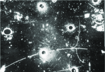
Figure 14: First $\nu_{\mu}e$ elastic scattering event observed by the Gargamelle Collaboration [10] at CERN. Muon neutrinos enter the Freon (CF₃Br) bubble chamber from the right. A recoiling electron appears near the center of the image and travels toward the left, initiating a shower of curling branches.

(see Figure 14).

To exercise your calculational muscles, please do

Problem 3

It’s an easy exercise to compute all the cross sections for neutrino-electron elastic scattering. Show that

$$\sigma(\nu_{\mu}e\to\nu_{\mu}e) = \displaystyle{\frac{G_{\mathrm{F}}^{2}m_{e}E_{\nu}}{2\pi}}\left[L_{e}^{2}+R_{e}^{2}/3\right]\;,$$

$$\sigma(\bar{\nu}_{\mu}e\to\bar{\nu}_{\mu}e) = \displaystyle{\frac{G_{\mathrm{F}}^{2}m_{e}E_{\nu}}{2\pi}}\left[L_{e}^{2}/3+R_{e}^{2}\right]\;,$$

$$\sigma(\nu_{e}e\to\nu_{e}e) = \displaystyle{\frac{G_{\mathrm{F}}^{2}m_{e}E_{\nu}}{2\pi}}\left[(L_{e}+2)^{2}+R_{e}^{2}/3\right]\;,$$

$$\sigma(\bar{\nu}_{e}e\to\bar{\nu}_{e}e) = \displaystyle{\frac{G_{\mathrm{F}}^{2}m_{e}E_{\nu}}{2\pi}}\left[(L_{e}+2)^{2}/3+R_{e}^{2}\right]\;.$$ (2.80)

By measuring all the cross sections, one may undertake a “model-independent” determination of the chiral couplings $L_{e}$ and $R_{e}$, or the traditional vector and axial-vector couplings $v$ and $a$, which are related through

$$\begin{array}[]{ccc}a=\cfrac{1}{2}(L_{e}-R_{e})&&v=\cfrac{1}{2}(L_{e}-R_{e})\\[3.0pt] L_{e}=v+a&&R_{e}=v-a\end{array}\;.$$ (2.81)

By inspecting (2.80), you can see that even after measuring all four cross sections, there remains a two-fold ambiguity: the same cross sections result if we interchange $R_{e}\leftrightarrow-R_{e}$, or, equivalently, $v\leftrightarrow a$. The ambiguity is resolved by measuring the forward-backward asymmetry in a reaction like $e^{+}e^{-}\to\mu^{+}\mu^{-}$ at energies well below the $Z^{0}$ mass. The asymmetry is proportional to $(L_{e}-R_{e})(L_{\mu}-R_{\mu})$, or to $a_{e}a_{\mu}$, and so resolves the sign ambiguity for $R_{e}$, or the $v$-$a$ ambiguity.

2.3.3 Electroweak Interactions of Quarks

To extend our theory to include the electroweak interactions of quarks, we observe that each generation consists of a left-handed doublet

$$\begin{array}[]{cccc}&I_{3}&Q&Y=2(Q-I_{3})\\[6.0pt] \mathsf{L}_{q}=\left(\begin{array}[]{c}u\\[3.0pt] d\end{array}\right)_{\mathrm{L}}&\begin{array}[]{c}+\cfrac{1}{2}\\[3.0pt] -\cfrac{1}{2}\end{array}&\begin{array}[]{c}+\cfrac{2}{3}\\[3.0pt] -\cfrac{1}{3}\end{array}&\cfrac{1}{3}\;,\end{array}$$ (2.82)

and two right-handed singlets,

$$\begin{array}[]{cccc}&I_{3}&Q&Y=2(Q-I_{3})\\[6.0pt] \begin{array}[]{c}\mathsf{R}_{u}=u_{\mathrm{R}}\\[3.0pt] \mathsf{R}_{d}=d_{\mathrm{R}}\end{array}&\begin{array}[]{c}0\\[3.0pt] 0\end{array}&\begin{array}[]{c}+\cfrac{2}{3}\\[3.0pt] -\cfrac{1}{3}\end{array}&\begin{array}[]{c}+\cfrac{4}{3}\\[3.0pt] -\cfrac{2}{3}\end{array}\;,\par\end{array}$$ (2.83)

Proceeding as before, we find the Lagrangian terms for the $W$-quark charged-current interaction,

$$\mathcal{L}_{W\mathrm{-quark}}=\frac{-g}{2\sqrt{2}}\left[\bar{u}_{e}\gamma^{\mu}(1-\gamma_{5})d\>W^{+}_{\mu}+\bar{d}\gamma^{\mu}(1-\gamma_{5})u\>W^{-}_{\mu}\right]\;,$$ (2.84)

which is identical in form to the leptonic charged-current interaction (2.65). Universality is ensured by the fact that the charged-current interaction is determined by the weak isospin of the fermions, and that both quarks and leptons come in doublets.

The neutral-current interaction is also equivalent in form to its leptonic counterpart, (2.76) and (2.77). We may write it compactly as

$$\mathcal{L}_{Z\mathrm{-quark}}=\frac{-g}{4\cos\theta_{W}}\sum_{i=u,d}\bar{q}_{i}\gamma^{\mu}\left[L_{i}(1-\gamma_{5})+R_{i}(1+\gamma_{5})\right]q_{i}\>Z_{\mu}\;,$$ (2.85)

where the chiral couplings are

$$L_{i} = \tau_{3}-2Q_{i}\sin^{2}\theta_{W}\;,$$

$$R_{i} = -2Q_{i}\sin^{2}\theta_{W}\;.$$ (2.86)

Again we find a quark-lepton universality in the form—but not the values—of the chiral couplings.

2.3.4 Trouble in Paradise

Until now, we have based our construction on the idealization that the $u\leftrightarrow d$ transition is of universal strength. The unmixed doublet

$$\left(\begin{array}[]{c}u\\ d\end{array}\right)_{\mathrm{L}}$$

does not quite describe our world. We attain a better description by replacing

$$\left(\begin{array}[]{c}u\\ d\end{array}\right)_{\mathrm{L}}\to\left(\begin{array}[]{c}u\\ d_{\theta}\end{array}\right)_{\mathrm{L}}\;,$$

where

$$d_{\theta}\equiv d\,\cos\theta_{C}+s\,\sin\theta_{C}\;,$$ (2.87)

with $\cos\theta_{C}=0.9736\pm 0.0010$. The change to the “Cabibbo-rotated” doublet perfects the charged-current interaction—at least up to small third-generation effects that we could easily incorporate—but leads to serious trouble in the neutral-current sector, for which the interaction now becomes

$$\mathcal{L}_{Z\mathrm{-quark}} = \frac{-g}{4\cos\theta_{W}}\>Z_{\mu}\left\{\bar{u}\gamma^{\mu}\left[L_{u}(1-\gamma_{5})+R_{u}(1+\gamma_{5})\right]u\right.$$ (2.88)

$$+\bar{d}\gamma^{\mu}\left[L_{d}(1-\gamma_{5})+R_{d}(1+\gamma_{5})\right]d\,\cos^{2}\theta_{C}$$

$$+\bar{s}\gamma^{\mu}\left[L_{d}(1-\gamma_{5})+R_{d}(1+\gamma_{5})\right]s\,\sin^{2}\theta_{C}$$

$$+\bar{d}\gamma^{\mu}\left[L_{d}(1-\gamma_{5})+R_{d}(1+\gamma_{5})\right]s\,\sin\theta_{C}\cos\theta_{C}$$

$$+\left.\bar{s}\gamma^{\mu}\left[L_{d}(1-\gamma_{5})+R_{d}(1+\gamma_{5})\right]d\,\sin\theta_{C}\cos\theta_{C}\right\}\;,$$

Until the discovery and systematic study of the weak neutral current, culminating in the heroic measurements made at LEP and the SLC, there was not enough knowledge to challenge the first three terms. The last two strangeness-changing terms were known to be poisonous, because many of the early experimental searches for neutral currents were fruitless searches for precisely this sort of interaction. Strangeness-changing neutral-current interactions are not seen at an impressively low level.

Only recently have Brookhaven Experiments 787 [13] and 939 [14] detected three candidates for the decay $K^{+}\to\pi^{+}\nu\bar{\nu}$,

and inferred a branching ratio ${\mathcal{B}}(K^{+}\to\pi^{+}\nu\bar{\nu})=1.47^{+1.30}_{-0.89}\times 10^{-10}$.

The good agreement between the standard-model prediction, ${\mathcal{B}}(K_{L}\to\mu^{+}\mu^{-})=0.77\pm 0.11\times 10^{-10}$ (through the process $K_{L}\to\gamma\gamma\to\mu^{+}\mu^{-}$), and experiment [15] leaves little room for a strangeness-changing neutral-current contribution:

that is easily normalized to the normal charged-current leptonic decay of the $K^{+}$:

The cure for this fatal disease was put forward by Glashow, Iliopoulos, and Maiani [16]. Expand the model of quarks to include two left-handed doublets,

$$\left(\begin{array}[]{c}\nu_{e}\\ e^{-}\end{array}\right)_{\mathrm{L}}\;\;\left(\begin{array}[]{c}\nu_{\mu}\\ \mu^{-}\end{array}\right)_{\mathrm{L}}\;\;\;\;\;\;\left(\begin{array}[]{c}u\\ d_{\theta}\end{array}\right)_{\mathrm{L}}\;\;\left(\begin{array}[]{c}c\\ s_{\theta}\end{array}\right)_{\mathrm{L}}\;,$$ (2.89)

where

$$s_{\theta}=s\,\cos\theta_{C}-d\,\sin\theta_{C}\;,$$ (2.90)

plus the corresponding right-handed singlets, $e_{\mathrm{R}}$, $\mu_{\mathrm{R}}$, $u_{\mathrm{R}}$, $d_{\mathrm{R}}$, $c_{\mathrm{R}}$, and $s_{\mathrm{R}}$. This required the introduction of the charmed quark, $c$, which had not yet been observed. By the addition of the second quark generation, the flavor-changing cross terms vanish in the $Z$-quark interaction, and we are left with:

which is flavor diagonal!

The generalization to $n$ quark doublets is straightforward. Let the charged-current interaction be

$$\mathcal{L}_{W\mathrm{-quark}}=\frac{-g}{2\sqrt{2}}\left[\bar{\Psi}\gamma^{\mu}(1-\gamma_{5}){\mathcal{O}}\Psi\>W^{+}_{\mu}+\mathrm{h.c.}\right]\;,$$ (2.91)

where the composite quark spinor is

$$\Psi=\left(\begin{array}[]{c}u\\ c\\ \vdots\\ \\ d\\ s\\ \vdots\end{array}\right)$$ (2.92)

and the flavor structure is contained in

$${\mathcal{O}}=\left(\begin{array}[]{cc}0&U\\ 0&0\end{array}\right)\;,$$ (2.93)

where $U$ is the unitary quark-mixing matrix. The weak-isospin contribution to the neutral-current interaction has the form

$$\mathcal{L}_{Z\mathrm{-quark}}^{\mathrm{iso}}=\frac{-g}{4\cos\theta_{W}}\bar{\Psi}\gamma^{\mu}(1-\gamma_{5})\left[{\mathcal{O}},{\mathcal{O}}^{\dagger}\right]\Psi\;.$$ (2.94)

Since the commutator

$$\left[{\mathcal{O}},{\mathcal{O}}^{\dagger}\right]=\left(\begin{array}[]{cc}I&0\\ 0&-I\end{array}\right)$$ (2.95)

the neutral-current interaction is flavor diagonal, and the weak-isospin piece is, as expected, proportional to $\tau_{3}$.

In general, the $n\times n$ quark-mixing matrix $U$ can be parametrized in terms of $n(n-1)/2$ real mixing angles and $(n-1)(n-2)/2$ complex phases, after exhausting the freedom to redefine the phases of quark fields. The $3\times 3$ case of three mixing angles and one phase, often called the Cabibbo–Kobayashi-Maskawa matrix, presaged the discovery of the third generation of quarks and leptons [17].

2.4 Precision Tests of the Electroweak Theory

In its simplest form, with the electroweak gauge symmetry broken by the Higgs mechanism, the $\mathrm{SU(2)}_{\mathrm{L}}\otimes\mathrm{U(1)}_{Y}$ theory has scored many qualitative successes: the prediction of neutral-current interactions, the necessity of charm, the prediction of the existence and properties of the weak bosons $W^{\pm}$ and $Z^{0}$. Over the past ten years, in great measure due to the beautiful experiments carried out at the $Z$ factories at CERN and SLAC, precision measurements have tested the electroweak theory as a quantum field theory [18, 19], at the one-per-mille level, as indicated in Table 1.

Table 1: Precision measurements at the $Z^{0}$ pole. (For sources of the data, see [2] and [20].)

$M_{Z}$	$91\,187.6\pm 2.1\hbox{ MeV}$
$\Gamma_{Z}$	$2\,495.2\pm 2.3\hbox{ MeV}$
$\sigma^{0}_{\mathrm{hadronic}}$	$41.540\pm 0.037\hbox{ nb}$
$\Gamma_{\mathrm{hadronic}}$	$1744.4\pm 2.0\hbox{ MeV}$
$\Gamma_{\mathrm{leptonic}}$	$83.984\pm 0.086\hbox{ MeV}$
$\Gamma_{\mathrm{invisible}}$	$499.0\pm 1.5\hbox{ MeV}$

A classic achievement of the $Z$ factories is the determination of the number of light neutrino species. If we define the invisible width of the $Z^{0}$ as

$$\Gamma_{\mathrm{invisible}}=\Gamma_{Z}-\Gamma_{\mathrm{hadronic}}-3\Gamma_{\mathrm{leptonic}}\;,$$ (2.96)

then we can compute the number of light neutrino species as

$$N_{\nu}=\Gamma_{\mathrm{invisible}}/\Gamma^{\mathrm{SM}}(Z\to\nu_{i}\bar{\nu}_{i})\;.$$ (2.97)

A typical current value is $N_{\nu}=2.994\pm 0.012$, in excellent agreement with the observation of light $\nu_{e}$, $\nu_{\mu}$, and $\nu_{\tau}$. A graphical indication that only three neutrino species are accessible as $Z^{0}$ decay products is given in Figure 15.

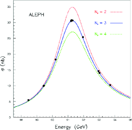
Figure 15: Comparison of the $Z^{0}$ line shape with predictions based on two, three, and four light neutrino species [21].

As an example of the insights precision measurements have brought us (one that mightily impressed the Royal Swedish Academy of Sciences in 1999), I show in Figure 16 the time evolution of the top-quark mass favored by simultaneous fits to many electroweak observables. Higher-order processes involving virtual top quarks are an important element in quantum corrections to the predictions the electroweak theory makes for many observables.

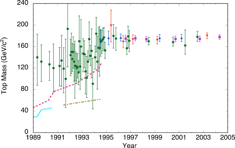
Figure 16: Indirect determinations of the top-quark mass from fits to electroweak observables (open circles) and 95% confidence-level lower bounds on the top-quark mass inferred from direct searches in $e^{+}e^{-}$ annihilations (solid line) and in $\bar{p}p$ collisions, assuming that standard decay modes dominate (broken line). An indirect lower bound, derived from the $W$-boson width inferred from $\bar{p}p\rightarrow(W\hbox{ or }Z)+\hbox{ anything}$, is shown as the dot-dashed line. Direct measurements of $m_{t}$ by the CDF (triangles) and DØ (inverted triangles) Collaborations are shown at the time of initial evidence, discovery claim, and at the conclusion of Run 1. The world averages from direct observations are shown as squares. For sources of data, see Ref. [2]. (From Ref. [22].)

A new world-average top mass has been reported by the Tevatron Collider experiments [23]: $m_{t}=178.0\pm 4.3\hbox{ GeV}$.

The comparison between the electroweak theory and a considerable universe of data is shown in Figure 17 where the pull, or difference between the global fit and measured value in units of standard deviations, is shown for some twenty observables [20].

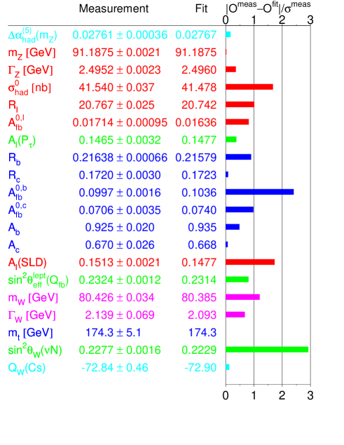
Figure 17: Precision electroweak measurements and the pulls they exert on a global fit to the standard model, from Ref. [20].

The distribution of pulls for this fit, due to the LEP Electroweak Working Group, is not noticeably different from a normal distribution, and only a couple of observables differ from the fit by as much as about two standard deviations. This is the case for any of the recent fits. From fits of the kind represented here, we learn that the standard-model interpretation of the data favors a light Higgs boson. We will revisit this conclusion in §2.9.

The beautiful agreement between the electroweak theory and a vast array of data from neutrino interactions, hadron collisions, and electron-positron annihilations at the $Z^{0}$ pole and beyond means that electroweak studies have become a modern arena in which we can look for new physics “in the sixth place of decimals.”

2.5 Why the Higgs boson must exist

How can we be sure that a Higgs boson, or something very like it, will be found? One path to the theoretical discovery of the Higgs boson involves its role in the cancellation of high-energy divergences. An illuminating example is provided by the reaction

Figure 18: Lowest-order contributions to the $e^{+}e^{-}\rightarrow W^{+}W^{-}$ scattering amplitude.

$e^{+}e^{-}\to W^{+}W^{-}$, which is described in lowest order by the four Feynman graphs in Figure 18. The contributions of the direct-channel $\gamma$- and $Z^{0}$-exchange diagrams of Figs. 18(a) and (b) cancel the leading divergence in the $J=1$ partial-wave amplitude of the neutrino-exchange diagram in Figure 18(c). This is the famous “gauge cancellation” observed in experiments at LEP 2 and the Tevatron. The LEP measurements in Figure 19

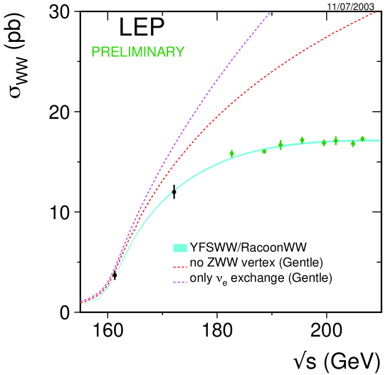
Figure 19: Cross section for the reaction $e^{+}e^{-}\to W^{+}W^{-}$ measured by the four LEP experiments, together with the full electroweak-theory simulation and the cross sections that would result from $\nu$-exchange alone and from $(\nu+\gamma)$-exchange [20]. .

agree well with the predictions of electroweak-theory Monte Carlo generators, which predict a benign high-energy behavior. If the $Z$-exchange contribution is omitted (middle dashed line) or if both the $\gamma$- and $Z$-exchange contributions are omitted (upper dashed line), the calculated cross section grows unacceptably with energy—and disagrees with the measurements. The gauge cancellation in the $J=1$ partial-wave amplitude is thus observed.

However, this is not the end of the high-energy story: the $J=0$ partial-wave amplitude, which exists in this case because the electrons are massive and may therefore be found in the “wrong” helicity state, grows as $s^{1/2}$ for the production of longitudinally polarized gauge bosons. The resulting divergence is precisely cancelled by the Higgs boson graph of Figure 18(d). If the Higgs boson did not exist, something else would have to play this role. From the point of view of $S$-matrix analysis, the Higgs-electron-electron coupling must be proportional to the electron mass, because “wrong-helicity” amplitudes are always proportional to the fermion mass.

Let us underline this result. If the gauge symmetry were unbroken, there would be no Higgs boson, no longitudinal gauge bosons, and no extreme divergence difficulties. But there would be no viable low-energy phenomenology of the weak interactions. The most severe divergences of individual diagrams are eliminated by the gauge structure of the couplings among gauge bosons and leptons. A lesser, but still potentially fatal, divergence arises because the electron has acquired mass—because of the Higgs mechanism. Spontaneous symmetry breaking provides its own cure by supplying a Higgs boson to remove the last divergence. A similar interplay and compensation must exist in any satisfactory theory.

2.6 The vacuum energy problem

I want to spend a moment to revisit a longstanding, but usually unspoken, challenge to the completeness of the electroweak theory as we have defined it: the vacuum energy problem [24, 25]. I do so not only for its intrinsic interest, but also to raise the question, “Which problems of completeness and consistency do we worry about at a given moment?” It is perfectly acceptable science—indeed, it is often essential—to put certain problems aside, in the expectation that we will return to them at the right moment. What is important is never to forget that the problems are there, even if we do not allow them to paralyze us.

For the usual Higgs potential, $V(\phi^{\dagger}\phi)=\mu^{2}(\phi^{\dagger}\phi)+\left|\lambda\right|(\phi^{\dagger}\phi)^{2}$, the value of the potential at the minimum is

$$V(\langle\phi^{\dagger}\phi\rangle_{0})=\frac{\mu^{2}v^{2}}{4}=-\frac{\left|\lambda\right|v^{4}}{4}<0.$$ (2.98)

Identifying $M_{H}^{2}=-2\mu^{2}$, we see that the Higgs potential contributes a field-independent constant term,

$$\varrho_{H}\equiv\frac{M_{H}^{2}v^{2}}{8}.$$ (2.99)

I have chosen the notation $\varrho_{H}$ because the constant term in the Lagrangian plays the role of a vacuum energy density. When we consider gravitation, adding a vacuum energy density $\varrho_{\mathrm{vac}}$ is equivalent to adding a cosmological constant term to Einstein’s equation. Although recent observations  raise the intriguing possibility that the cosmological constant may be different from zero (see Figure 20), the

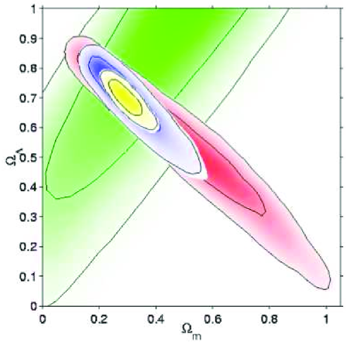
Figure 20: Constraints on the mass ($\Omega_{m}$) and dark-energy ($\Omega_{\Lambda}$) densities of the universe, at 68% and 95% confidence levels. Bottom layer (green): supernova constraints; next layer up (red): CMB data alone; next (blue): CMB data plus HST Key Project prior; top layer (yellow): all data combined [28].

essential observational fact is that the vacuum energy density must be very tiny indeed,

$$\varrho_{\mathrm{vac}}\mathop{\raisebox{-1.72218pt}{\hbox to0.0pt{$\sim$\hss}}\raisebox{1.72218pt}{$<$}}10^{-46}\hbox{ GeV}^{4}\;.$$ (2.100)

Therein lies the puzzle: if we take $v=(G_{\mathrm{F}}\sqrt{2})^{-\frac{1}{2}}\approx 246\hbox{ GeV}$ and insert the current experimental lower bound [29] $M_{H}\mathop{\raisebox{-1.72218pt}{\hbox to0.0pt{$\sim$\hss}}\raisebox{1.72218pt}{$>$}}114.4\hbox{ GeV}$ into (2.99), we find that the contribution of the Higgs field to the vacuum energy density is

$$\varrho_{H}\mathop{\raisebox{-1.72218pt}{\hbox to0.0pt{$\sim$\hss}}\raisebox{1.72218pt}{$>$}}10^{8}\hbox{ GeV}^{4},$$ (2.101)

some 54 orders of magnitude larger than the upper bound inferred from the cosmological constant.

What are we to make of this mismatch? The fact that $\varrho_{H}\gg\varrho_{\mathrm{vac}}$ means that the smallness of the cosmological constant needs to be explained. In a unified theory of the strong, weak, and electromagnetic interactions, other (heavy!) Higgs fields have nonzero vacuum expectation values that may give rise to still greater mismatches. At a fundamental level, we can therefore conclude that a spontaneously broken gauge theory of the strong, weak, and electromagnetic interactions—or merely of the electroweak interactions—cannot be complete. Either we must find a separate principle to zero the vacuum energy density of the Higgs field, or we may suppose that a proper quantum theory of gravity, in combination with the other interactions, will resolve the puzzle of the cosmological constant. The vacuum energy problem must be an important clue. But to what?

2.7 Bounds on $M_{H}$

The Standard Model does not give a precise prediction for the mass of the Higgs boson. We can, however, use arguments of self-consistency to place plausible lower and upper bounds on the mass of the Higgs particle in the minimal model. Unitarity arguments [30] lead to a conditional upper bound on the Higgs boson mass. It is straightforward to compute the amplitudes ${\cal M}$ for gauge boson scattering at high energies, and to make a partial-wave decomposition, according to

$${\cal M}(s,t)=16\pi\sum_{J}(2J+1)a_{J}(s)P_{J}(\cos{\theta})\;.$$ (2.102)

Most channels “decouple,” in the sense that partial-wave amplitudes are small at all energies (except very near the particle poles, or at exponentially large energies), for any value of the Higgs boson mass $M_{H}$. Four channels are interesting:

$$\begin{array}[]{cccc}W_{L}^{+}W_{L}^{-}&Z_{L}^{0}Z_{L}^{0}/\sqrt{2}&HH/\sqrt{2}&HZ_{L}^{0}\;,\end{array}$$ (2.103)

where the subscript $L$ denotes the longitudinal polarization states, and the factors of $\sqrt{2}$ account for identical particle statistics. For these channels, the $s$-wave amplitudes are all asymptotically constant (i.e., well-behaved) and proportional to $G_{\mathrm{F}}M_{H}^{2}.$ In the high-energy limit,

$$\lim_{s\gg M_{H}^{2}}(a_{0})\to\frac{-G_{\mathrm{F}}M_{H}^{2}}{4\pi\sqrt{2}}\cdot\left[\begin{array}[]{cccc}1&1/\sqrt{8}&1/\sqrt{8}&0\\ 1/\sqrt{8}&3/4&1/4&0\\ 1/\sqrt{8}&1/4&3/4&0\\ 0&0&0&1/2\end{array}\right]\;.$$ (2.104)

Requiring that the largest eigenvalue respect the partial-wave unitarity condition $\left|a_{0}\right|\leq 1$ yields

$$M_{H}\leq\left(\frac{8\pi\sqrt{2}}{3G_{\mathrm{F}}}\right)^{1/2}=1\hbox{ TeV}$$ (2.105)

as a condition for perturbative unitarity.

If the bound is respected, weak interactions remain weak at all energies, and perturbation theory is everywhere reliable. If the bound is violated, perturbation theory breaks down, and weak interactions among $W^{\pm}$, $Z$, and $H$ become strong on the 1-TeV scale. This means that the features of strong interactions at GeV energies will come to characterize electroweak gauge boson interactions at TeV energies. We interpret this to mean that new phenomena are to be found in the electroweak interactions at energies not much larger than 1 TeV.

Lower bounds on the Higgs mass that follow from the requirement that electroweak symmetry be broken in the vacuum, even in the presence of quantum corrections, date from the work of Linde [33] and Weinberg [34]. The effects of heavy fermions—important for the top quark—are explored in [35, 36, 37].

2.8 The electroweak scale and beyond

We have seen that the scale of electroweak symmetry breaking, $v=(G_{\mathrm{F}}\sqrt{2})^{-\frac{1}{2}}\approx 246\hbox{ GeV}$, sets the values of the $W$- and $Z$-boson masses. But the electroweak scale is not the only scale of physical interest. It seems certain that we must also consider the Planck scale, derived from the strength of Newton’s constant, and it is also probable that we must take account of the $\mathrm{SU(3)_{c}}\otimes\mathrm{SU(2)}_{\mathrm{L}}\otimes\mathrm{U(1)}_{Y}$ unification scale around $10^{15\mathrm{-}16}\hbox{ GeV}$. There may well be a distinct flavor scale. The existence of other significant energy scales is behind the famous problem of the Higgs scalar mass: how to keep the distant scales from mixing in the face of quantum corrections, or how to stabilize the mass of the Higgs boson on the electroweak scale, or why is the electroweak scale small? We call this puzzle the hierarchy problem.

The $\mathrm{SU(2)}_{\mathrm{L}}\otimes\mathrm{U(1)}_{Y}$ electroweak theory does not explain how the scale of electroweak symmetry breaking is maintained in the presence of quantum corrections. The problem of the scalar sector can be summarized neatly as follows [38, 39]. The Higgs potential is

$$V(\phi^{\dagger}\phi)=\mu^{2}(\phi^{\dagger}\phi)+\left|\lambda\right|(\phi^{\dagger}\phi)^{2}\;.$$ (2.106)

With $\mu^{2}$ chosen to be less than zero, the electroweak symmetry is spontaneously broken down to the $\mathrm{U(1)}$ of electromagnetism, as the scalar field acquires a vacuum expectation value that is fixed by the low-energy phenomenology,

$$\langle\phi\rangle_{0}=\sqrt{-\mu^{2}/2|\lambda|}\equiv(G_{\mathrm{F}}\sqrt{8})^{-1/2}\approx 174{\rm\;GeV}\;.$$ (2.107)

Beyond the classical approximation, scalar mass parameters receive quantum corrections from loops that contain particles of spins $J=1,1/2$, and $0$:

(2.108)

The loop integrals are potentially divergent. Symbolically, we may summarize the content of (2.108) as

$$m^{2}(p^{2})=m^{2}(\Lambda^{2})+Cg^{2}\int^{\Lambda^{2}}_{p^{2}}dk^{2}+\cdots\;,$$ (2.109)

where $\Lambda$ defines a reference scale at which the value of $m^{2}$ is known, $g$ is the coupling constant of the theory, and the coefficient $C$ is calculable in any particular theory. Instead of dealing with the relationship between observables and parameters of the Lagrangian, we choose to describe the variation of an observable with the momentum scale. In order for the mass shifts induced by radiative corrections to remain under control (i.e., not to greatly exceed the value measured on the laboratory scale), either $\Lambda$ must be small, so the range of integration is not enormous, or new physics must intervene to cut off the integral.

If the fundamental interactions are described by an $\mathrm{SU(3)_{c}}\otimes\mathrm{SU(2)}_{\mathrm{L}}\otimes\mathrm{U(1)}_{Y}$ gauge symmetry, i.e., by quantum chromodynamics and the electroweak theory, then the natural reference scale is the Planck mass,

$$\Lambda\sim M_{\rm Planck}=\left(\frac{\hbar c}{G_{\mathrm{Newton}}}\right)^{1/2}\approx 1.22\times 10^{19}{\rm\;GeV}\;.$$ (2.110)

In a unified theory of the strong, weak, and electromagnetic interactions, the natural scale is the unification scale,

$$\Lambda\sim U\approx 10^{15}\hbox{-}10^{16}{\rm\;GeV}\;.$$ (2.111)

Both estimates are very large compared to the scale of electroweak symmetry breaking (2.107). We are therefore assured that new physics must intervene at an energy of approximately 1 TeV, in order that the shifts in $m^{2}$ not be much larger than (2.107).

2.9 Clues to the Higgs-boson mass

We have seen in our discussion of Figure 16 that the sensitivity of electroweak observables to the (long unknown) mass of the top quark gave early indications for a very massive top. For example, the quantum corrections to the standard-model predictions given below (2.64) for $M_{W}$ and $M_{Z}$ arise from different quark loops:

$t\bar{b}$ for $M_{W}$, and $t\bar{t}$ (or $b\bar{b}$) for $M_{Z}$. These quantum corrections alter the link between the $W$- and $Z$-boson masses, so that

$$M_{W}^{2}=M_{Z}^{2}\left(1-\sin^{2}\theta_{W}\right)\left(1+\Delta\rho\right)\;,$$ (2.112)

where

$$\Delta\rho\approx\Delta\rho^{(\mathrm{quarks})}=\frac{3G_{\mathrm{F}}m_{t}^{2}}{8\pi^{2}\sqrt{2}}\;.$$ (2.113)

The strong dependence on $m_{t}^{2}$ is characteristic, and it accounts for the precision of the top-quark mass estimates derived from electroweak observables.

Now that $m_{t}$ is known to about 2.5% from direct observations at the Tevatron, it becomes profitable to look beyond the quark loops to the next most important quantum corrections, which arise from Higgs-boson effects. The Higgs-boson quantum corrections are typically smaller than the top-quark corrections, and exhibit a more subtle dependence on $M_{H}$ than the $m_{t}^{2}$ dependence of the top-quark corrections. For the case at hand,

$$\Delta\rho^{\mathrm{(Higgs)}}=\mathsf{C}\cdot\ln\left(\frac{M_{H}}{v}\right)\;,$$ (2.114)

where I have arbitrarily chosen to define the coefficient $\mathsf{C}$ at the electroweak scale $v$.

Figure 21 shows how the goodness of the

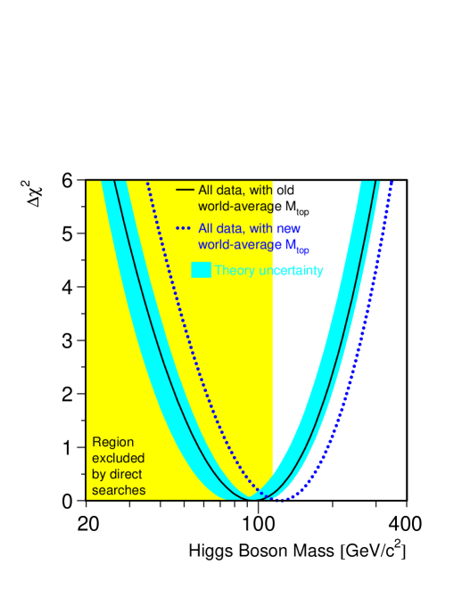
Figure 21: $\Delta\chi^{2}=\chi^{2}-\chi^{2}_{\mathrm{min}}$ from a global fit to precision data vs. the Higgs-boson mass, $M_{H}$. The solid line is the result of the fit with $m_{t}=174.3\hbox{ GeV}$; the band represents an estimate of the theoretical error due to missing higher order corrections. The yellow-shaded region shows the 95% CL exclusion limit on $M_{H}$ from the direct search at LEP. The dashed curve shows the change brought about by the new Tevatron average top mass, $m_{t}=178.0\hbox{ GeV}$. (From Ref. [20].) .

LEP Electroweak Working Group’s global fit depends upon the Higgs-boson mass. Within the standard model, they deduce a 95% CL upper limit, $M_{H}\mathop{\raisebox{-1.72218pt}{\hbox to0.0pt{$\sim$\hss}}\raisebox{1.72218pt}{$<$}}219(251)\hbox{ GeV}$, for $m_{t}=174.3\pm 5.1(178.0\pm 4.3)\hbox{ GeV}$. The recent increase in the world-average top mass changes the best-fit Higgs-boson mass from $96^{+60}_{-38}\hbox{ GeV}$ to $117^{+67}_{-45}\hbox{ GeV}$. The direct searches at LEP have concluded that $M_{H}>114.4\hbox{ GeV}$ [29], excluding much of the favored region. Even with the additional breathing space afforded by a higher top mass, either the Higgs boson is just around the corner, or the standard-model analysis is misleading. Things will soon be popping!

We will begin to explore the new physics that may lie beyond the standard model in Lecture 3, where we take up the possibility of unified theories of the strong, weak, and electromagnetic interactions. Let us conclude today’s rapid survey of the electroweak theory by summarizing some of the questions we have encountered:

Second Harvest of Questions

• What contrives a Higgs potential that hides electroweak symmetry?

• What separates the electroweak scale from higher scales?

• What are the distinct scales of physical interest?

• Why is empty space so nearly weightless?

• What determines the gauge symmetries?

• What accounts for the range of fermion masses?

• Why is (strong-interaction) isospin a good symmetry? What does it mean?

To prepare for our discussion of unified theories, please review the elements of group theory and work out

Problem 4

Examine the (standard-model) $\mathrm{SU(3)_{c}}\otimes\mathrm{SU(2)}_{\mathrm{L}}\otimes\mathrm{U(1)}_{Y}$ content of the 5, 10, and 24 representations of $\mathrm{SU(5)}$. Decompose the fundamental 16 and adjoint 45 representations of $\mathrm{SO(10)}$ into $\mathrm{{SU(5)}\otimes U(1)}$; into $\mathrm{{SU(4)}\otimes{SU(2)}\otimes{SU(2)}}$.

3 Unified Theories

REDES 239: Los Ladrillos del Universo $\cdot$ 19.5.2002 $\cdot$ TVE

Eduardo Punset: Una teoría acerca de todo? Chris Quigg: Bueno, no me gusta la expresión de teoría acerca del todo, porque incluso después de conocer todas las reglas todavía queda por saber cómo aplicar esas reglas a este maravilloso mundo tan diverso y complejo que nos rodea. Por tanto, creo que deberíamos tener un poco más de humildad cuando utilizamos expresiones como esa de “teoría acerca del todo”, pero es una teoría de “mucho”.

Eduardo Punset: A theory of everything? Chris Quigg: I don’t like the expression, “a theory of everything,” because even if we should ever know all the rules, we still must learn how to apply those rules to this marvelous world of diversity and change that surrounds us. For that reason, I believe we should display a little more humility when we use expressions like “theory of everything.” Nevertheless, it is a theory of quite a lot!

3.1 Why Unify?

The standard model based on $\mathrm{SU(3)_{c}}\otimes\mathrm{SU(2)}_{\mathrm{L}}\otimes\mathrm{U(1)}_{Y}$ gauge symmetry encapsulates much of what we know and describes many observations, but it leaves many things unexplained. Both the success and the incompleteness of the standard model encourage us to look beyond it to a more comprehensive understanding. One attractive way to proceed is by enlarging the gauge group, which we may attempt either by accreting F9 new symmetries or by unifying the symmetries we have already recognized.

Left-right symmetric models, such as those based on the gauge symmetry

$$\mathrm{SU(3)_{c}\otimes SU(2)_{L}\otimes SU(2)_{R}\otimes U(1)}_{B-L}\;,$$

follow the first path. Such models attribute the observed parity violation in the weak interactions to spontaneous symmetry breaking—the $\mathrm{SU(2)_{R}}$ symmetry is broken at a higher scale than the $\mathrm{SU(2)_{L}}$—and naturally accommodate Majorana neutrinos. We saw in Lecture 1 that they can be represented readily in the double simplex. Left-right symmetric theories also open new possibilities, including transitions that induce $n\leftrightarrow\bar{n}$ oscillations and a mechanism for spontaneous $\mathcal{CP}$ violation. More generally, enlarging the gauge group by accretion seeks to add a missing element or to explain additional observations.

Unified theories, on the other hand, seek to find a symmetry group

$${\mathcal{G}}\supset\mathrm{SU(3)_{c}}\otimes\mathrm{SU(2)}_{\mathrm{L}}\otimes\mathrm{U(1)}_{Y}$$

(usually a simple group, to maximize the predictive power) that contains the known interactions. This approach is motivated by the desire to unify quarks and leptons and to reduce the number of independent coupling constants, the better to understand the relative strengths of the strong, weak, and electromagnetic interactions at laboratory energies. Supersymmetric unified theories, which we will investigate briefly in Lecture 4, bring the added ambitions of incorporating gravity and joining constituents and forces.

Two very potent ideas are at play here. The first is the idea of unification itself: what Feynman calls amalgamation, which is the central notion of generalization and synthesis that scientific explanation represents. Examples from the history of physics include Maxwell’s joining of electricity and magnetism and light; the atomic hypothesis, which places thermodynamics and statistical mechanics within the realm of Newtonian mechanics; and the links among atomic structure, chemistry, and quantum mechanics.

The second is the notion that the human scale of space and time is not privileged for understanding Nature, and may even be disadvantaged. Not only in physics, but throughout science, this has been a growing recognition since the quantum-mechanical revolution of the 1920s. To understand why a rock is solid, or why a metal gleams, we must understand its structure on a scale a billion times smaller $(10^{-9})$ than the human scale, and we must understand the rules that prevail there. It may well be that certain scales are privileged for understanding certain globally important aspects of the Universe: why, for example, the fine structure constant $\alpha\approx 1/137$, and why the strong coupling, measured at the $B$ factories is $\alpha_{s}\approx 1/5$; or why fermion masses have the (seemingly unintelligible) pattern they do.

I believe that the discovery that the human scale is not preferred is as important as the discoveries that the human location is not privileged (Copernicus) and that there is no preferred inertial frame (Einstein), and will prove to be as influential.

Let us examine the motivation for constructing a unified theory in greater detail. $\Box$ Quarks and leptons are structureless, spin-$\cfrac{1}{2}$ particles. (How) are they related? $\Box$ What is the meaning of electroweak universality, embodied in the matching left-handed doublets of quarks and leptons? $\Box$ Anomaly cancellation requires quarks and leptons. $\Box$ Can the three distinct coupling parameters of the standard model ($\alpha_{s},\alpha_{\mathrm{em}},\sin^{2}\theta_{W}$ or $g_{s},g,g^{\prime}$) be reduced to two or one? $\Box$ $\alpha_{\mathrm{em}}$ increases with $Q^{2}$; $\alpha_{s}$ decreases. Is there a unification point where all (suitably defined) couplings coincide? $\Box$ Why is charge quantized? [$Q_{d}=\cfrac{1}{3}Q_{e}$, $Q_{p}+Q_{e}=0$, $Q_{\nu}-Q_{e}=Q_{u}-Q_{d}$, $Q_{\nu}+Q_{e}+3Q_{u}+3Q_{d}=0$.]

These questions lead us toward a more complete electroweak unification, which is to say a simple $\mathcal{G}\supset\mathrm{SU(2)}_{\mathrm{L}}\otimes\mathrm{U(1)}_{Y}$; a quark-lepton connection; a “grand” unification of the strong, weak, and electromagnetic interactions, based on a simple group $\mathcal{G}\supset\mathrm{SU(3)_{c}}\otimes\mathrm{SU(2)}_{\mathrm{L}}\otimes\mathrm{U(1)}_{Y}$. If we choose the task of grand unification, we must find a group that contains the known interactions and that can accommodate the known fermions—either as one generation plus replicas, or as all three generations at once. The unifying group will surely contain interactions beyond the established ones, and we should be open to the possibility that the fermion representations require the existence of particles yet undiscovered.

3.2 Toward a Unified Theory

It is convenient to express all the fermions in terms of left-handed fields, for ease in counting degrees of freedom. Denoting the quantum numbers as $(\mathrm{SU(3)_{c},SU(2)_{L}})_{Y}$, we can enumerate the fermions of the first generation as follows:

$$\begin{array}[]{rl}u_{\mathrm{L}},d_{\mathrm{L}}:&(\mathbf{3},\mathbf{2})_{1/3}\\ d^{c}_{\mathrm{L}}:&(\mathbf{3^{*}},\mathbf{1})_{2/3}\\ u^{c}_{\mathrm{L}}:&(\mathbf{3^{*}},\mathbf{1})_{-4/3}\\ \nu_{\mathrm{L}},e_{\mathrm{L}}:&(\mathbf{1},\mathbf{2})_{-1}\\ e^{c}_{\mathrm{L}}:&(\mathbf{1},\mathbf{1})_{2}\\ {\nu^{c}_{\mathrm{L}}:}&{(\mathbf{1},\mathbf{1})_{0}}\;.\end{array}$$ (3.1)

This collection of particles is not identical to its conjugate, so $\mathcal{G}$ must admit complex representations. The smallest appropriate group is $\mathrm{SU(5)}$, and we shall choose it to illustrate the strategy of unified theories.

Let us examine the low-dimensional representations of $\mathrm{SU(5)}$. The fundamental representation is

$\hbox{}\vbox{\vbox{\offinterlineskip\vbox{\hrule height=0.3pt\hbox{\vrule height=8.74669pt,width=0.3pt,depth=2.18663pt\hbox to10.93333pt{\hfil}\vrule height=8.74669pt,width=0.3pt,depth=2.18663pt} \hrule height=0.3pt}\vspace{-\y@linethick} }}\quad\mathbf{5}=(\mathbf{3},\mathbf{1})_{-2/3}\oplus(\mathbf{1},\mathbf{2})_{1}$,

and its conjugate is

$\hbox{}\vbox{\vbox{\offinterlineskip\vbox{\hrule height=0.3pt\hbox{\vrule height=8.74669pt,width=0.3pt,depth=2.18663pt\hbox to10.93333pt{\hfil}\vrule height=8.74669pt,width=0.3pt,depth=2.18663pt} \hrule height=0.3pt}\vspace{-\y@linethick} \vbox{\hrule height=0.3pt\hbox{\vrule height=8.74669pt,width=0.3pt,depth=2.18663pt\hbox to10.93333pt{\hfil}\vrule height=8.74669pt,width=0.3pt,depth=2.18663pt} \hrule height=0.3pt}\vspace{-\y@linethick} \vbox{\hrule height=0.3pt\hbox{\vrule height=8.74669pt,width=0.3pt,depth=2.18663pt\hbox to10.93333pt{\hfil}\vrule height=8.74669pt,width=0.3pt,depth=2.18663pt} \hrule height=0.3pt}\vspace{-\y@linethick} \vbox{\hrule height=0.3pt\hbox{\vrule height=8.74669pt,width=0.3pt,depth=2.18663pt\hbox to10.93333pt{\hfil}\vrule height=8.74669pt,width=0.3pt,depth=2.18663pt} \hrule height=0.3pt}\vspace{-\y@linethick} }}\quad\mathbf{5^{*}}=(\mathbf{3^{*}},\mathbf{1})_{2/3}\oplus(\mathbf{1},\mathbf{2})_{-1}$.

To generate larger representations, we consider products of the fundamental, for example

$\mathbf{5}\otimes\mathbf{5}$ : $\hbox{}\vbox{\vbox{\offinterlineskip\vbox{\hrule height=0.3pt\hbox{\vrule height=8.74669pt,width=0.3pt,depth=2.18663pt\hbox to10.93333pt{\hfil}\vrule height=8.74669pt,width=0.3pt,depth=2.18663pt} \hrule height=0.3pt}\vspace{-\y@linethick} }}\otimes\hbox{}\vbox{\vbox{\offinterlineskip\vbox{\hrule height=0.3pt\hbox{\vrule height=8.74669pt,width=0.3pt,depth=2.18663pt\hbox to10.93333pt{\hfil}\vrule height=8.74669pt,width=0.3pt,depth=2.18663pt} \hrule height=0.3pt}\vspace{-\y@linethick} }}=\hbox{}\vbox{\vbox{\offinterlineskip\vbox{\hrule height=0.3pt\hbox{\vrule height=8.74669pt,width=0.3pt,depth=2.18663pt\hbox to10.93333pt{\hfil}\vrule height=8.74669pt,width=0.3pt,depth=2.18663pt} \hrule height=0.3pt}\vspace{-\y@linethick} \vbox{\hrule height=0.3pt\hbox{\vrule height=8.74669pt,width=0.3pt,depth=2.18663pt\hbox to10.93333pt{\hfil}\vrule height=8.74669pt,width=0.3pt,depth=2.18663pt} \hrule height=0.3pt}\vspace{-\y@linethick} }}\oplus\hbox{}\vbox{\vbox{\offinterlineskip\vbox{\hrule height=0.3pt\hbox{\vrule height=8.74669pt,width=0.3pt,depth=2.18663pt\hbox to10.93333pt{\hfil}\vrule height=8.74669pt,width=0.3pt,depth=2.18663pt\hbox to10.93333pt{\hfil}\vrule height=8.74669pt,width=0.3pt,depth=2.18663pt} \hrule height=0.3pt}\vspace{-\y@linethick} }}=\mathbf{10}\oplus\mathbf{15}$,

where

$$\mathbf{15}=(\mathbf{6},\mathbf{1})_{-4/3}\oplus(\mathbf{3},\mathbf{2})_{1/3}\oplus(\mathbf{1},\mathbf{3})_{2}\;,$$

and

$$\mathbf{10}=(\mathbf{3^{*}},\mathbf{1})_{-4/3}\oplus(\mathbf{3},\mathbf{2})_{1/3}\oplus(\mathbf{1},\mathbf{1})_{2}\;.$$

The product of the fundamental with its conjugate is

$\mathbf{5}\otimes\mathbf{5^{*}}$ : $\hbox{}\vbox{\vbox{\offinterlineskip\vbox{\hrule height=0.3pt\hbox{\vrule height=8.74669pt,width=0.3pt,depth=2.18663pt\hbox to10.93333pt{\hfil}\vrule height=8.74669pt,width=0.3pt,depth=2.18663pt} \hrule height=0.3pt}\vspace{-\y@linethick} }}\otimes\hbox{}\vbox{\vbox{\offinterlineskip\vbox{\hrule height=0.3pt\hbox{\vrule height=8.74669pt,width=0.3pt,depth=2.18663pt\hbox to10.93333pt{\hfil}\vrule height=8.74669pt,width=0.3pt,depth=2.18663pt} \hrule height=0.3pt}\vspace{-\y@linethick} \vbox{\hrule height=0.3pt\hbox{\vrule height=8.74669pt,width=0.3pt,depth=2.18663pt\hbox to10.93333pt{\hfil}\vrule height=8.74669pt,width=0.3pt,depth=2.18663pt} \hrule height=0.3pt}\vspace{-\y@linethick} \vbox{\hrule height=0.3pt\hbox{\vrule height=8.74669pt,width=0.3pt,depth=2.18663pt\hbox to10.93333pt{\hfil}\vrule height=8.74669pt,width=0.3pt,depth=2.18663pt} \hrule height=0.3pt}\vspace{-\y@linethick} \vbox{\hrule height=0.3pt\hbox{\vrule height=8.74669pt,width=0.3pt,depth=2.18663pt\hbox to10.93333pt{\hfil}\vrule height=8.74669pt,width=0.3pt,depth=2.18663pt} \hrule height=0.3pt}\vspace{-\y@linethick} }}=\hbox{}\vbox{\vbox{\offinterlineskip\vbox{\hrule height=0.3pt\hbox{\vrule height=8.74669pt,width=0.3pt,depth=2.18663pt\hbox to10.93333pt{\hfil}\vrule height=8.74669pt,width=0.3pt,depth=2.18663pt} \hrule height=0.3pt}\vspace{-\y@linethick} \vbox{\hrule height=0.3pt\hbox{\vrule height=8.74669pt,width=0.3pt,depth=2.18663pt\hbox to10.93333pt{\hfil}\vrule height=8.74669pt,width=0.3pt,depth=2.18663pt} \hrule height=0.3pt}\vspace{-\y@linethick} \vbox{\hrule height=0.3pt\hbox{\vrule height=8.74669pt,width=0.3pt,depth=2.18663pt\hbox to10.93333pt{\hfil}\vrule height=8.74669pt,width=0.3pt,depth=2.18663pt} \hrule height=0.3pt}\vspace{-\y@linethick} \vbox{\hrule height=0.3pt\hbox{\vrule height=8.74669pt,width=0.3pt,depth=2.18663pt\hbox to10.93333pt{\hfil}\vrule height=8.74669pt,width=0.3pt,depth=2.18663pt} \hrule height=0.3pt}\vspace{-\y@linethick} \vbox{\hrule height=0.3pt\hbox{\vrule height=8.74669pt,width=0.3pt,depth=2.18663pt\hbox to10.93333pt{\hfil}\vrule height=8.74669pt,width=0.3pt,depth=2.18663pt} \hrule height=0.3pt}\vspace{-\y@linethick} }}\oplus\hbox{}\vbox{\vbox{\offinterlineskip\vbox{\hrule height=0.3pt\hbox{\vrule height=8.74669pt,width=0.3pt,depth=2.18663pt\hbox to10.93333pt{\hfil}\vrule height=8.74669pt,width=0.3pt,depth=2.18663pt\hbox to10.93333pt{\hfil}\vrule height=8.74669pt,width=0.3pt,depth=2.18663pt} \hrule height=0.3pt}\vspace{-\y@linethick} \vbox{\hrule height=0.3pt\hbox{\vrule height=8.74669pt,width=0.3pt,depth=2.18663pt\hbox to10.93333pt{\hfil}\vrule height=8.74669pt,width=0.3pt,depth=2.18663pt} \hrule height=0.3pt}\vspace{-\y@linethick} \vbox{\hrule height=0.3pt\hbox{\vrule height=8.74669pt,width=0.3pt,depth=2.18663pt\hbox to10.93333pt{\hfil}\vrule height=8.74669pt,width=0.3pt,depth=2.18663pt} \hrule height=0.3pt}\vspace{-\y@linethick} \vbox{\hrule height=0.3pt\hbox{\vrule height=8.74669pt,width=0.3pt,depth=2.18663pt\hbox to10.93333pt{\hfil}\vrule height=8.74669pt,width=0.3pt,depth=2.18663pt} \hrule height=0.3pt}\vspace{-\y@linethick} }}=\mathbf{1}\oplus\mathbf{24}$,

where

$${\mathbf{1}=(\mathbf{1},\mathbf{1})_{0}}\;,$$

and

$$\mathbf{24}=\mathbf{24^{*}}={(\mathbf{8},\mathbf{1})_{0}}\,\oplus{(\mathbf{3},\mathbf{2})_{-5/3}}\,\oplus{(\mathbf{3^{*}},\mathbf{2})_{5/3}}\,\oplus{(\mathbf{1},\mathbf{3})_{0}}\oplus{(\mathbf{1},\mathbf{1})_{0}}\;.$$

Finally, consider the product

$\mathbf{5}\otimes\mathbf{10^{*}}$ : $\hbox{}\vbox{\vbox{\offinterlineskip\vbox{\hrule height=0.3pt\hbox{\vrule height=8.74669pt,width=0.3pt,depth=2.18663pt\hbox to10.93333pt{\hfil}\vrule height=8.74669pt,width=0.3pt,depth=2.18663pt} \hrule height=0.3pt}\vspace{-\y@linethick} }}\otimes\hbox{}\vbox{\vbox{\offinterlineskip\vbox{\hrule height=0.3pt\hbox{\vrule height=8.74669pt,width=0.3pt,depth=2.18663pt\hbox to10.93333pt{\hfil}\vrule height=8.74669pt,width=0.3pt,depth=2.18663pt} \hrule height=0.3pt}\vspace{-\y@linethick} \vbox{\hrule height=0.3pt\hbox{\vrule height=8.74669pt,width=0.3pt,depth=2.18663pt\hbox to10.93333pt{\hfil}\vrule height=8.74669pt,width=0.3pt,depth=2.18663pt} \hrule height=0.3pt}\vspace{-\y@linethick} \vbox{\hrule height=0.3pt\hbox{\vrule height=8.74669pt,width=0.3pt,depth=2.18663pt\hbox to10.93333pt{\hfil}\vrule height=8.74669pt,width=0.3pt,depth=2.18663pt} \hrule height=0.3pt}\vspace{-\y@linethick} }}=\hbox{}\vbox{\vbox{\offinterlineskip\vbox{\hrule height=0.3pt\hbox{\vrule height=8.74669pt,width=0.3pt,depth=2.18663pt\hbox to10.93333pt{\hfil}\vrule height=8.74669pt,width=0.3pt,depth=2.18663pt} \hrule height=0.3pt}\vspace{-\y@linethick} \vbox{\hrule height=0.3pt\hbox{\vrule height=8.74669pt,width=0.3pt,depth=2.18663pt\hbox to10.93333pt{\hfil}\vrule height=8.74669pt,width=0.3pt,depth=2.18663pt} \hrule height=0.3pt}\vspace{-\y@linethick} \vbox{\hrule height=0.3pt\hbox{\vrule height=8.74669pt,width=0.3pt,depth=2.18663pt\hbox to10.93333pt{\hfil}\vrule height=8.74669pt,width=0.3pt,depth=2.18663pt} \hrule height=0.3pt}\vspace{-\y@linethick} \vbox{\hrule height=0.3pt\hbox{\vrule height=8.74669pt,width=0.3pt,depth=2.18663pt\hbox to10.93333pt{\hfil}\vrule height=8.74669pt,width=0.3pt,depth=2.18663pt} \hrule height=0.3pt}\vspace{-\y@linethick} }}\oplus\hbox{}\vbox{\vbox{\offinterlineskip\vbox{\hrule height=0.3pt\hbox{\vrule height=8.74669pt,width=0.3pt,depth=2.18663pt\hbox to10.93333pt{\hfil}\vrule height=8.74669pt,width=0.3pt,depth=2.18663pt\hbox to10.93333pt{\hfil}\vrule height=8.74669pt,width=0.3pt,depth=2.18663pt} \hrule height=0.3pt}\vspace{-\y@linethick} \vbox{\hrule height=0.3pt\hbox{\vrule height=8.74669pt,width=0.3pt,depth=2.18663pt\hbox to10.93333pt{\hfil}\vrule height=8.74669pt,width=0.3pt,depth=2.18663pt} \hrule height=0.3pt}\vspace{-\y@linethick} \vbox{\hrule height=0.3pt\hbox{\vrule height=8.74669pt,width=0.3pt,depth=2.18663pt\hbox to10.93333pt{\hfil}\vrule height=8.74669pt,width=0.3pt,depth=2.18663pt} \hrule height=0.3pt}\vspace{-\y@linethick} }}=\mathbf{5^{*}}\oplus\mathbf{45^{*}}$,

where

$$\mathbf{45^{*}}=(\mathbf{8},\mathbf{2})_{-1}\oplus(\mathbf{6},\mathbf{1})_{2/3}\oplus(\mathbf{3^{*}},\mathbf{3})_{2/3}\oplus(\mathbf{3},\mathbf{2})_{7/3}\oplus(\mathbf{3^{*}},\mathbf{1})_{2/3}\oplus(\mathbf{3},\mathbf{1})_{-8/3}\oplus(\mathbf{1},\mathbf{2})_{-1}\;.$$

Now we look for a fit. $\Box$ Does a generation (without a right-handed neutrino) fit in the 15-dimensional representation? It does not: $\mathbf{15}=(\mathbf{6},\mathbf{1})_{-4/3}\oplus(\mathbf{3},\mathbf{2})_{1/3}\oplus(\mathbf{1},\mathbf{3})_{2}$ contains color-sextet quarks! $\Box$ Do three generations fit in the 45-dimensional representation? No, $\mathbf{45^{*}}=(\mathbf{8},\mathbf{2})_{-1}\oplus(\mathbf{6},\mathbf{1})_{2/3}\oplus(\mathbf{3^{*}},\mathbf{3})_{2/3}\oplus(\mathbf{3},\mathbf{2})_{7/3}\oplus(\mathbf{3^{*}},\mathbf{1})_{2/3}\oplus(\mathbf{3},\mathbf{1})_{-8/3}\oplus(\mathbf{1},\mathbf{2})_{-1}$ contains color-octet and color-sextet fermions. $\Box$ If nothing fits like a glove, perhaps we should try a glove and a mitten, placing one generation in several representations, $\mathbf{5^{*}}\,\oplus\mathbf{10}\,\oplus\mathbf{1}$:

$$\begin{array}[]{rlc}{u_{L},d_{L}:}&{(\mathbf{3},\mathbf{2})_{1/3}}&{\mathbf{10}}\\ {d^{c}_{L}:}&{(\mathbf{3^{*}},\mathbf{1})_{2/3}}&{\mathbf{5^{*}}}\\ {u^{c}_{L}:}&{(\mathbf{3^{*}},\mathbf{1})_{-4/3}}&{\mathbf{10}}\\ {\nu_{L},e_{L}:}&{(\mathbf{1},\mathbf{2})_{-1}}&{\mathbf{5^{*}}}\\ {e^{c}_{L}:}&{(\mathbf{1},\mathbf{1})_{2}}&{\mathbf{10}}\\ {\nu^{c}_{L}:}&{(\mathbf{1},\mathbf{1})_{0}}&{\mathbf{1}}\end{array}$$

The presence of both quarks and leptons in either the $\mathbf{5^{*}}$ or $\mathbf{10}$ means that we can expect quark-lepton transformations.

What about the gauge interactions? The twelve known gauge bosons fit in the adjoint $\mathbf{24}$ representation:

$$\begin{array}[]{cc}(\mathbf{8},\mathbf{1})_{0}&\hbox{gluons}\\ (\mathbf{1},\mathbf{3})_{0}&W^{\pm},W_{3}\\ (\mathbf{1},\mathbf{1})_{0}&\mathcal{A}\;.\end{array}\hbox{ or }(b_{1},b_{2},b_{3})$$

The $\mathbf{24}$ also includes new fractionally charged leptoquark gauge bosons

$$\begin{array}[]{ll}(\mathbf{3},\mathbf{2})_{-5/3}&X^{-4/3},Y^{-1/3}\\ (\mathbf{3^{*}},\mathbf{2})_{5/3}&X^{4/3},Y^{1/3}\end{array}$$

that mediate the transitions illustrated in Figure 22.

Figure 22: Transitions mediated by the $X^{\pm 4/3}$ and $Y^{\pm 1/3}$ gauge bosons in the $\mathrm{SU(5)}$ unified theory.

Recall that the price (or reward!) of the partial electroweak unification achieved in the $\mathrm{SU(2)}_{\mathrm{L}}\otimes\mathrm{U(1)}_{Y}$ theory was a new interaction, the weak neutral current. Here again we find that new interactions are required to complete the symmetry—just as our geometrical discussion in Lecture 1 invited us to think.

The new vertices of Figure 22 can give rise to proton decay, which is known to be an exceedingly rare process. Accordingly, we must arrange that $X^{\pm 4/3}$ and $Y^{\pm 1/3}$ acquire very large masses, lest the proton decay rapidly. We hide the $\mathrm{SU(5)}$ symmetry in two steps. First, a $\mathbf{24}$ of auxiliary scalars breaks $\mathrm{SU(5)}\to\mathrm{SU(3)_{c}}\otimes\mathrm{SU(2)}_{\mathrm{L}}\otimes\mathrm{U(1)}_{Y}$ at a high scale, to give large masses to $X^{\pm 4/3}$ and $Y^{\pm 1/3}$. The $\mathbf{24}$ does not occur in the $\bar{\mathsf{L}}\mathsf{R}$ products

$$\mathbf{5}^{\ast}\otimes\mathbf{10} = \mathbf{5}\oplus\mathbf{45}$$ (3.2)

$$\mathbf{10}\otimes\mathbf{10} = \mathbf{5}^{\ast}\oplus\mathbf{45}^{\ast}\oplus\mathbf{50}^{\ast}$$

that generate fermion masses, so the quarks and leptons escape large tree-level masses. At a second stage, a $\mathbf{5}$ of scalars containing the standard-model Higgs fields breaks $\mathrm{SU(3)_{c}}\otimes\mathrm{SU(2)}_{\mathrm{L}}\otimes\mathrm{U(1)}_{Y}\to\mathrm{SU(3)_{c}}\otimes\mathrm{U(1)}_{\mathrm{em}}$.

The $\mathrm{SU(5)}$ unification brings a pair of agreeable consequences. If built on a complete generation of quarks and leptons, the theory is anomaly free, which guarantees that the symmetries survive quantum corrections. The anomalies of the $\mathbf{5^{*}}$ and $\mathbf{10}$ representations are equal and opposite, $A(\mathbf{5^{*}})=-1$, $A(\mathbf{10})=+1$, while $A(\mathbf{1})=0$, so that $A(\mathbf{5^{*}})+A(\mathbf{10})=0$. If this seems a little precarious, we can note that $\mathrm{SO(10)}$ representations are anomaly free, and that $\mathrm{SO(10)}\;\mathbf{16}=\mathbf{10}\oplus\mathbf{5^{*}}\oplus\mathbf{1}\hbox{ of }\mathrm{SU(5)}$. In addition, the unified theory offers us an explanation of charge quantization. Because the charge operator $Q$ is a generator of $\mathrm{SU(5)}$, the charges must sum to zero in any representation. Applied to the $\mathbf{5^{*}}$, we find that $Q(d^{c})=-\cfrac{1}{3}Q(e)$, one of the quark-lepton “coincidences” we wish to understand.

3.3 The Interaction Lagrangian and Running Couplings

The $\mathrm{SU(5)}$ unified theory is based on a simple group, so the strength of all the gauge interactions is specified by a single coupling constant, $g_{5}$. The theory prescribes the relative normalization of the electroweak theory’s independent couplings, $g$ and $g^{\prime}$, and predicts the weak mixing parameter

$$\sin^{2}\theta_{W}=\displaystyle{\frac{g^{\prime\,2}}{g^{2}+g^{\prime\,2}}}\;.$$ (3.3)

Let us see how this coupling-constant concordance comes about. The $\mathrm{SU(5)}$ interaction Lagrangian is

$$\mathcal{L}_{\mathrm{int}} = -\frac{g_{5}}{2}G_{\mu}^{a}\left(\bar{u}\gamma^{\mu}\lambda^{a}u+\bar{d}\gamma^{\mu}\lambda^{a}d\right)$$

$$-\frac{g_{5}}{2}W_{\mu}^{i}\left(\bar{\mathsf{L}}_{u}\gamma^{\mu}\tau^{i}\mathsf{L}_{u}+\bar{\mathsf{L}}_{e}\gamma^{\mu}\tau^{i}\mathsf{L}_{e}\right)$$

$$-\frac{g_{5}}{2}{\sqrt{\cfrac{3}{5}}}\mathcal{A}_{\mu}\sum_{\mathrm{fermions}}\bar{f}\gamma^{\mu}Yf$$

$$+X\hbox{ and }Y\hbox{ pieces}\;,$$

where, in a familiar notation,

$$\mathsf{L}_{u}=\left(\begin{array}[]{c}u\\ d_{\theta}\end{array}\right)_{\mathrm{L}}\quad\mathsf{L}_{e}=\left(\begin{array}[]{c}\nu_{e}\\ e\end{array}\right)_{\mathrm{L}}\;.$$ (3.5)

In the weak-hypercharge piece, the factor $\sqrt{\cfrac{3}{5}}$ arises from the form of the normalized generator in $\mathrm{SU(5)}$,

$$\cfrac{1}{\sqrt{30}}\left(\begin{array}[]{ccccc}-2&&&&\\ &-2&&0&\\ &&-2&&\\ &0&&3&\\ &&&&3\end{array}\right)\propto Y\;.$$ (3.6)

In electroweak terms, we identify

$$g^{\prime\,2}=\cfrac{3}{5}g^{2}\;,$$ (3.7)

so that in unbroken $\mathrm{SU(5)}$, we predict

$${\sin^{2}\theta_{W}=\frac{g^{\prime\,2}}{g^{2}+g^{\prime\,2}}=\frac{\cfrac{3}{5}}{1+\cfrac{3}{5}}=\frac{3}{8}}\;.$$ (3.8)

We carry out experiments at low energies, whereas if $\mathrm{SU(5)}$ is the unifying symmetry it is unbroken at extremely high energies. To make the connection, we need to examine the evolution of coupling constants—the dependence on energy scale that occurs in quantum field theory. Below a possible unification scale, the $\mathrm{SU(3)_{c}}\otimes\mathrm{SU(2)}_{\mathrm{L}}\otimes\mathrm{U(1)}_{Y}$ coupling constants evolve separately. In leading-logarithmic approximation, we have

$$\mathrm{SU(3)_{\mathrm{c}}:}\quad 1/\alpha_{3}(Q^{2})=1/\alpha_{3}(\mu^{2})+b_{3}\log(Q^{2}/\mu^{2})\;,$$ (3.9)

where $4\pi b_{3}=11-4n_{\mathrm{gen}}/3$, so that $b_{3}=7/4\pi$;

$$\mathrm{SU(2)_{\mathrm{L}}:}\quad 1/\alpha_{2}(Q^{2})=1/\alpha_{2}(\mu^{2})+b_{2}\log(Q^{2}/\mu^{2})\;,$$ (3.10)

where $4\pi b_{2}=(22-4n_{\mathrm{gen}})/3-n_{\mathrm{Higgs}}/6$, so that $b_{2}=19/24\pi$; and

$$\mathrm{U(1)}_{Y}:\quad 1/\alpha_{1}(Q^{2})=1/\alpha_{Y}(\mu^{2})+b_{1}\log(Q^{2}/\mu^{2})\;,$$ (3.11)

with $4\pi b_{1}=-4n_{\mathrm{gen}}/3-n_{\mathrm{Higgs}}/10$, so that $b_{1}=-41/40\pi$. In (3.9)–(3.11), $Q^{2}$ is the scale of interest and $\mu^{2}$ is the reference scale.

Running couplings are not merely an artifact of quantum field theory, they are observed! Figure 23 shows the evolution of the strong coupling constant as determined by the CDF collaboration from their study of $\bar{p}p\to\hbox{jets}$ [41].

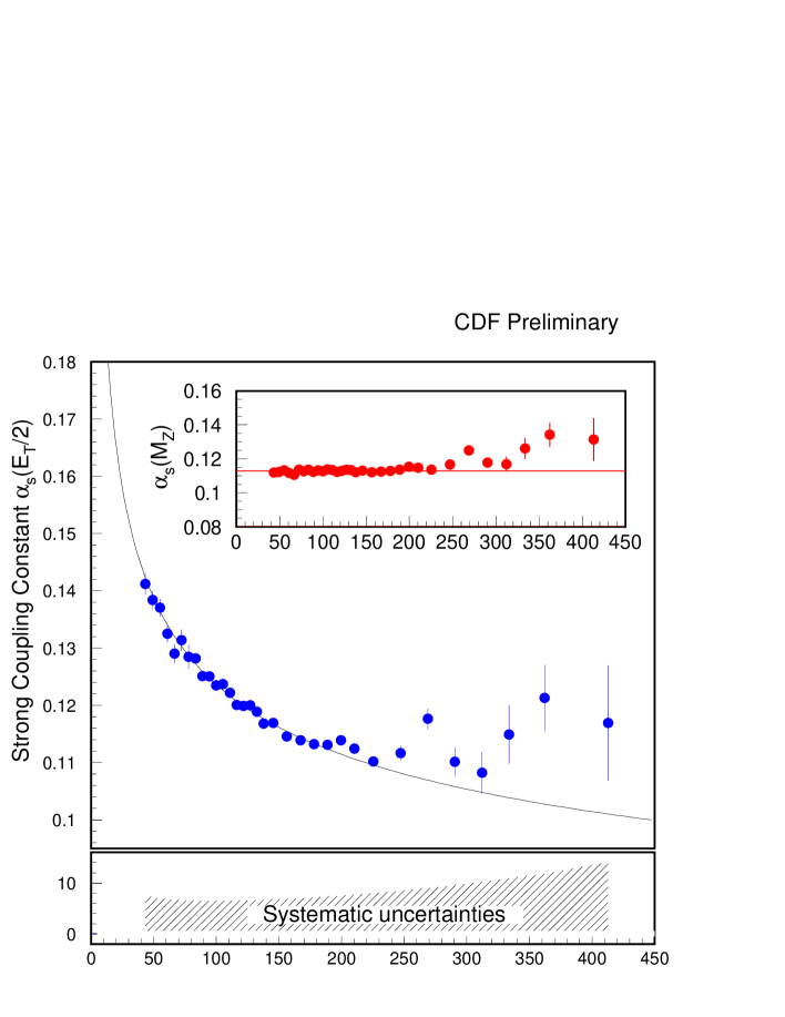
Figure 23: Evolution of the strong coupling constant $\alpha_{s}(E_{T}/2)$ measured in jet studies at $1.8\hbox{ TeV}$ [41]. The curve shows the expectations from QCD. The inset shows the values measured at different values of $E_{T}$ evolved to the $Z$-boson mass.

A little easier to visualize is the compilation [2] plotted in Figure 24 as $1/\alpha_{s}$ over a wide range of energies. There the goodness of the form (3.9) is readily apparent.

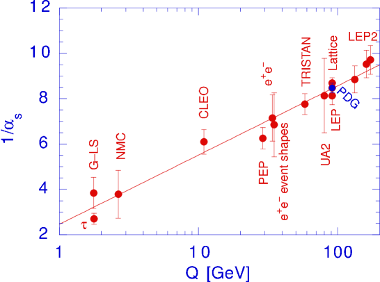
Figure 24: Running of $1/\alpha_{s}(Q)$ determined in a variety of experiments at different energies. The point labeled PDG is the world-average value, presented at the $Z$-boson mass.

Having recalled the expectations for how coupling “constants” run, we can check the prediction of $\mathrm{SU(5)}$ unification. We recall that the electromagnetic coupling in the electroweak theory is a derived quantity that we can express in terms of the $\mathrm{SU(2)_{L}}$ and weak-hypercharge couplings as

$$1/\alpha(Q^{2})\equiv 1/\alpha_{Y}(Q^{2})+1/\alpha_{2}(Q^{2})\;,$$ (3.12)

where $\alpha_{Y}$ is proportional to $\alpha_{1}$. Relating the couplings to the $\mathrm{SU(5)}$ coupling $\alpha_{U}$ at the unification scale $U$, we have

$$1/\alpha(Q^{2})=\cfrac{8}{3}\cdot 1/\alpha_{U}+({b_{Y}}+{b_{2}})\log({Q^{2}}/{U^{2}})\;,$$ (3.13)

which suggests that we form

$$\displaystyle{\frac{({8}/{3})}{\alpha_{s}(Q^{2})}}-\frac{1}{\alpha(Q^{2})} = \underbrace{\left(\displaystyle{\frac{8{b_{3}}}{3}}-{b_{Y}}-{b_{2}}\right)}\log(\frac{Q^{2}}{U^{2}})$$

$$\frac{22+n_{\mathrm{Higgs}}}{4\pi}\rightarrow\frac{67}{12\pi}\;.$$

Using the measured values, $\alpha_{3}(M_{Z}^{2})\approx 1/8.75$, $\alpha(M_{Z}^{2})\approx 1/128.9$, and $M_{Z}\approx 91.19\hbox{ GeV}$, we can use (3.3) to estimate $U\approx 10^{15}\hbox{ GeV}$ and $1/\alpha_{U}\approx 42$.

Now we are ready to test $\mathrm{SU(5)}$ unification using the weak mixing parameter

$$x_{W}\equiv\sin^{2}\theta_{W}=\alpha/\alpha_{2}=\frac{1/\alpha_{2}}{1/\alpha_{Y}+1/\alpha_{2}}\;.$$ (3.15)

At the unification scale, the running couplings are simply related:

$$\left.\begin{array}[]{l}1/\alpha_{2}=1/\alpha_{U}\\ 1/\alpha_{Y}=\cfrac{5}{3}\cdot 1/\alpha_{U}\\ 1/\alpha=\cfrac{8}{3}\cdot 1/\alpha_{U}\end{array}\right\}\;,$$ (3.16)

so that ${x_{W}(U^{2})=\cfrac{3}{8}}$, as we have already noticed in (3.8). How does $x_{W}$ evolve? Putting together the pieces, we find that

$$x_{W}(Q^{2})=\cfrac{3}{8}-\underbrace{\cfrac{5}{8}(b_{1}-b_{2})}_{+109/96\pi}\alpha(Q^{2})\log\left(Q^{2}/U^{2}\right)\;,$$ (3.17)

which decreases as $Q$ decreases from the unification scale $U$, as sketched in Figure 25.

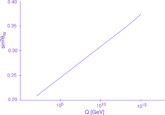
Figure 25: Running of $\sin^{2}\theta_{W}$ in the $\mathrm{SU(5)}$ unified theory.

At the $Z$-boson mass, we calculate

$$\left.x_{W}(M_{Z}^{2})\right|_{\mathrm{SU(5)}}\approx 0.21\;,$$ (3.18)

to be compared with the measured value,

$$\left.x_{W}(M_{Z}^{2})\right|_{\mathrm{exp}}=0.2314\pm 0.003\;.$$ (3.19)

So near, and yet so far!

An equivalent way to display the same information is to combine the measured $\alpha_{1}(M_{Z}^{2})\approx 1/60$ with $\alpha(M_{Z}^{2})\approx 1/128.9$ to determine $\alpha_{2}(M_{Z}^{2})\approx 1/30$, and then to evolve $1/\alpha_{1},1/\alpha_{2},1/\alpha_{3}$ to high energies to see whether they meet. As we can anticipate from the near miss of $x_{W}$, the three couplings do not quite coincide at a single point at high energy, though they come close in the neighborhood of $10^{14\pm 1}\hbox{ GeV}$, as plotted in Figure 26. [With six Higgs doublets, they do coincide!]

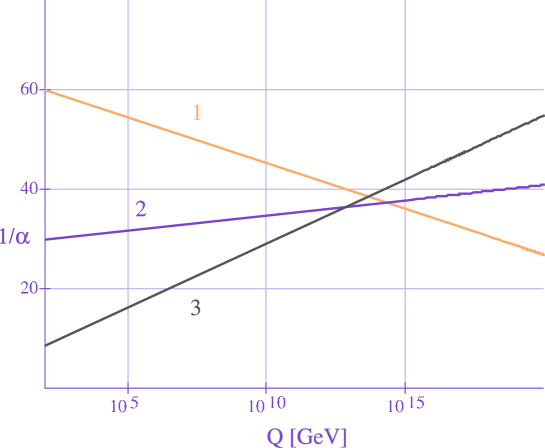
Figure 26: Running of $1/\alpha_{1},1/\alpha_{2},1/\alpha_{3}$ in the $\mathrm{SU(5)}$ unified theory.

Problem 5

Suppose that a unified theory, $\mathrm{SU(5)}$ for definiteness, fixes the value of the unification scale, $U$, and the strength of the couplings, $1/\alpha_{U}$, at that scale. The value of the coupling constants that we measure on a low scale have encrypted in them information about the spectrum of particles between our energy scale and $U$. Assume that there are no particles in that range beyond those we know from the standard model. How is the strong coupling constant $\alpha_{s}$ at low energies influenced by the mass of the top quark? What is the effect on the proton mass?

This problem is a lovely example of the influence on the commonplace of phenomena that we study far from the realm of everyday experience, so I will provide a brief answer. First, it is easy to see, by referring to (3.9) for the evolution of $1/\alpha_{s}$ (which means $1/\alpha_{3}$) that the slope of $1/\alpha_{s}$ changes from $21/6\pi$ to $23/6\pi$ when we descend through top threshold, and decreased by another $2/6\pi$ at every succeeding threshold. Without doing any arithmetic, we can sketch the evolution of $1/\alpha_{s}$ for two values of the top-quark mass, as I have done in Figure 27:

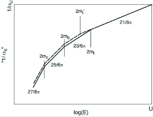
Figure 27: Running of the strong coupling constant $1/\alpha_{s}$ for two values of $m_{t}$ in the $\mathrm{SU(5)}$ unified theory.

the smaller the value of $m_{t}$, the smaller the value of $\alpha_{s}$.

To determine the effect of varying the top-quark mass on the mass of the proton, we apply the lesson of (lattice) QCD that the mass of the proton is mostly determined by the energy stored up in the gluon field that confines three light quarks in a small volume. To good approximation, therefore, we can write the proton mass in terms of the QCD scale parameter as

$$M_{\mathrm{proton}}\approx C\Lambda_{\mathrm{QCD}}\;,$$ (3.20)

where the constant $C$ could be determined by lattice simulations. How, then, does $\Lambda_{\mathrm{QCD}}$ depend on $m_{t}$? We calculate $\alpha_{s}(2m_{t})$ evolving up from low energies and down from the unification scale, and match:

$$\begin{array}[]{l}1/\alpha_{U}+{\displaystyle\frac{21}{6\pi}}\ln(2m_{t}/M_{U})=\\ \quad 1/\alpha_{s}(2m_{c})-{\displaystyle\frac{25}{6\pi}}\ln(m_{c}/m_{b})-{\displaystyle\frac{23}{6\pi}}\ln(m_{b}/m_{t})\;.\end{array}$$ (3.21)

Using the convenient three-active-flavor definition

$$1/\alpha_{s}(2m_{c})\equiv{\displaystyle\frac{27}{6\pi}}\ln(2m_{c}/\Lambda_{\mathrm{QCD}})\;,$$ (3.22)

we solve for

$$\Lambda_{\mathrm{QCD}}=\hbox{constants}\cdot\left(\frac{2m_{t}\cdot 2m_{b}\cdot 2m_{c}}{(1\hbox{ GeV})^{3}}\right)^{\!2/27}\hbox{ GeV}\;.$$ (3.23)

The variation of $\Lambda_{\mathrm{QCD}}$ with the top-quark mass is shown in Figure 28.

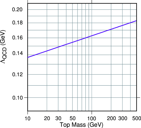
Figure 28: Dependence of the QCD scale parameter $\Lambda_{\mathrm{QCD}}$ on $m_{t}$ in the $\mathrm{SU(5)}$ unified theory.

With this, we have our answer. Although the population of top-antitop pairs within the proton is vanishingly small, because of the top quark’s great mass, virtual effects of the top quark do affect the strong coupling constant we measure at low energies, within the framework of a unified theory. The proton mass is proportional to $(m_{t}/1\hbox{ GeV})^{2/27}$, for reasonable variations of $m_{t}$. This knowledge is of no conceivable technological value, but I find it utterly wonderful—the kind of below-the-surface connection that makes it such a delight to be a physicist!

3.4 The Problem of Fermion Masses

Unraveling the origins of electroweak symmetry breaking will not necessarily give insight into the origin and pattern of fermion masses, because they are set by the Yukawa couplings $\zeta_{i},$ of unknown provenance, that we first met in (2.24). The puzzling pattern of quark masses is depicted in Figure 29.

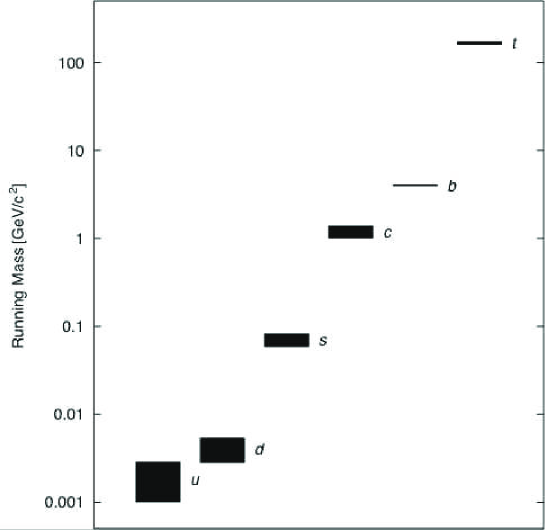
Figure 29: Running ($\overline{\mathrm{MS}}$) masses of the quarks. The heavy-quark ($c,b,t$) masses are evaluated at the quark masses, $\overline{m}_{q}(m_{q})$, while the light-quark masses ($u,d,s$) are evaluated at $1\hbox{ GeV}$.

The fact that masses—like coupling constants—are scale-dependent might encourage us to hope that what looks like an irrational pattern at low scales will reveal an underlying order at some other scale.

To illustrate the possibilities, let us adopt the specific framework of $\mathrm{SU(5)}$ unification, with the two-step spontaneously symmetry breaking we introduced in § 3.2. At a high scale, a $\mathbf{24}$ of scalars breaks $\mathrm{SU(5)}\to\mathrm{SU(3)_{c}}\otimes\mathrm{SU(2)}_{\mathrm{L}}\otimes\mathrm{U(1)}_{Y}$, giving extremely large masses to the leptoquark gauge bosons $X^{\pm 4/3}$ and $Y^{\pm 1/3}$. As we have already observed, the $\mathbf{24}$ does not occur in the $\bar{\mathsf{L}}\mathsf{R}$ products that generate fermion masses, so quarks and leptons escape large tree-level masses. At the electroweak scale, a $\mathbf{5}$ of scalars ($\supset$ the standard-model Higgs fields) breaks $\mathrm{SU(3)_{c}}\otimes\mathrm{SU(2)}_{\mathrm{L}}\otimes\mathrm{U(1)}_{Y}\to\mathrm{SU(3)}_{\mathrm{c}}\otimes U(1)_{\mathrm{em}}$, and endows fermions with mass. This approach relates quark and lepton masses at the unification scale,

$${\left.\begin{array}[]{c}m_{e}=m_{d}\\ m_{\mu}=m_{s}\\ m_{\tau}=m_{b}\end{array}\right\}\mbox{ at }U\;;}{\mbox{ separate parameters }\left\{\begin{array}[]{l}m_{u}\\ m_{c}\\ m_{t}\;,\end{array}\right.}$$ (3.24)

with implications for the observed masses that we will now elaborate.

The fermion masses evolve from the unification scale $U$ to the experimental scale $\mu$:

$$\ln\left[m_{u,c,t}(\mu)\right] \approx \ln\left[m_{u,c,t}(U)\right]+{\frac{12}{33-2n_{f}}\ln\left(\frac{\alpha_{3}(\mu)}{\alpha_{U}}\right)}$$

$$+{\frac{27}{88-8n_{f}}\ln\left(\frac{\alpha_{2}(\mu)}{\alpha_{U}}\right)}-{\frac{3}{10n_{f}}\ln\left(\frac{\alpha_{1}(\mu)}{\alpha_{U}}\right)}\;,$$

$$\ln\left[m_{d,s,b}(\mu)\right] \approx \ln\left[m_{d,s,b}({U})\right]+{\frac{12}{33-2n_{f}}\ln\left(\frac{\alpha_{3}(\mu)}{\alpha_{U}}\right)}$$

$$+{\frac{27}{88-8n_{f}}\ln\left(\frac{\alpha_{2}(\mu)}{\alpha_{U}}\right)}+{\frac{3}{20n_{f}}\ln\left(\frac{\alpha_{1}(\mu)}{\alpha_{U}}\right)}\;,$$

$$\ln\left[m_{e,\mu,\tau}(\mu)\right] \approx \ln\left[m_{e,\mu,\tau}({U})\right]\phantom{+{\frac{12}{33-2n_{f}}\ln\left(\frac{\alpha_{3}(\mu)}{\alpha_{U}}\right)}}$$

$$+{\frac{27}{88-8n_{f}}\ln\left(\frac{\alpha_{2}(\mu)}{\alpha_{U}}\right)}-{\frac{27}{20n_{f}}\ln\left(\frac{\alpha_{1}(\mu)}{\alpha_{U}}\right)}\;,$$

where I have omitted a small Higgs-boson contribution to keep the formulas short. The classic success of $\mathrm{SU(5)}$ unification is the predicted relation between $m_{b}$ and $m_{\tau}$ [42]. Combining (3.4) and (3.4), we have

$$\ln\left[\frac{m_{b}(\mu)}{m_{\tau}(\mu)}\right]\approx{\ln\left[\frac{m_{b}({U})}{m_{\tau}({U})}\right]}+{\frac{12}{33-2n_{f}}\ln\left(\frac{\alpha_{3}(\mu)}{\alpha_{U}}\right)}-{\frac{3}{2n_{f}}\ln\left(\frac{\alpha_{1}(\mu)}{\alpha_{U}}\right)}\;,$$ (3.28)

where the first term on the right-hand side vanishes. Choosing for illustration $n_{f}=6$, $1/\alpha_{U}=40$, $1/\alpha_{s}(\mu)=5$, and $1/\alpha_{1}(\mu)=65$, we compute at a low scale

$$m_{b}=2.91m_{\tau}\approx 5.16\hbox{ GeV}\;,$$ (3.29)

in suggestive agreement with experiment. The factor-of-three ratio arises because the quark masses, influenced by QCD, evolve more rapidly than the lepton masses.

The example of $b$-$\tau$ unification raises the hope that all fermion masses arise on high scales, and show simple patterns there. The other cases are not so pretty. You can see the situation yourself by working

Problem 6

Choosing an observation scale $\mu\approx 1\hbox{ GeV}$, compute $m_{s}/m_{\mu}$ and $m_{d}/m_{e}$ and compare with experiment. A more elaborate symmetry breaking scheme that adds a $\mathbf{45}$ of scalars can change the relation for $m_{e}/m_{d}$ at the unification scale, and lead to a more agreeable result at low energies. Show that the relations $m_{s}=\cfrac{1}{3}m_{\mu}$, $m_{d}=3m_{e}$ at the unification scale lead to the low-energy predictions, $m_{s}\approx\cfrac{4}{3}m_{\mu}$ and $m_{d}\approx 12m_{e}$.

The prospect of finding order among the fermion masses has spawned a lively theoretical industry.  The essential strategy comprises four steps: $\Box$ Begin with supersymmetric $\mathrm{SU(5)}$, which has advantages (as we shall see in Lecture 4) for $\sin^{2}\theta_{W}$, coupling-constant unification, and the proton lifetime, or with supersymmetric $\mathrm{SO(10)}$, which accommodates a massive neutrino gracefully. $\Box$ Find “textures”—simple patterns of Yukawa matrices—that lead to successful predictions for masses and mixing angles. $\Box$ Interpret the textures in terms of symmetry breaking patterns. $\Box$ Seek a derivation—or at least a motivation—for the winning entry.

Aside: varieties of neutrino mass. We recall that the chiral decomposition of a Dirac spinor is

$$\psi={\scriptstyle\frac{1}{2}}(1-\gamma_{5})\psi+{\scriptstyle\frac{1}{2}}(1+\gamma_{5})\psi\equiv\psi_{\mathrm{L}}+\psi_{\mathrm{R}}\;,$$ (3.30)

and that the charge conjugate of a right-handed field is left-handed, $\psi_{\mathrm{L}}^{c}\equiv(\psi^{c})_{\mathrm{L}}=(\psi_{\mathrm{R}})^{c}$. What are the possible forms for mass terms? The familiar Dirac mass term, as we have emphasized for the quarks and charged leptons, connects the left-handed and right-handed components of the same field,

$$\mathcal{L}_{\mathrm{D}}=D(\bar{\psi}_{\mathrm{L}}\psi_{\mathrm{R}}+\bar{\psi}_{\mathrm{R}}\psi_{\mathrm{L}})=D\bar{\psi}\psi\;,$$ (3.31)

(compare (1.3)) so that the mass eigenstate is $\psi=\psi_{\mathrm{L}}+\psi_{\mathrm{R}}$. This combination is invariant under global phase rotation $\nu\rightarrow e^{i\theta}\nu$, $\ell\rightarrow e^{i\theta}\ell$, so that lepton number is conserved.

In contrast, Majorana mass terms connect the left-handed and right-handed components of conjugate fields,

$$-\mathcal{L}_{\mathrm{MA}} = A(\bar{\psi}_{\mathrm{R}}^{c}\psi_{\mathrm{L}}+\bar{\psi}_{\mathrm{L}}\psi_{\mathrm{R}}^{c})=A\bar{\chi}\chi$$

$$-\mathcal{L}_{\mathrm{MB}} = B(\bar{\psi}^{c}_{\mathrm{L}}\psi_{\mathrm{R}}+\bar{\psi}_{\mathrm{R}}\psi^{c}_{\mathrm{L}})=B\bar{\omega}\omega\;,$$ (3.32)

which is only possible for neutral fields. In the Majorana case, the mass eigenstates are

$$\chi \equiv \psi_{\mathrm{L}}+\psi^{c}_{\mathrm{R}}=\chi^{c}=\psi_{\mathrm{L}}+(\psi_{\mathrm{L}})^{c}$$

$$\omega \equiv \psi_{\mathrm{R}}+\psi^{c}_{\mathrm{L}}=\omega^{c}=\psi_{\mathrm{R}}+(\psi_{\mathrm{R}})^{c}\;.$$ (3.33)

The mixing of particle and antiparticle fields means that the Majorana mass terms correspond to processes that violate lepton number by two units. Accordingly, a Majorana neutrino can mediate neutrinoless double beta decay, $(Z,A)\rightarrow(Z+2,A)+e^{-}+e^{-}$. Detecting neutrinoless double beta decay would offer decisive evidence for the Majorana nature of the neutrino.

Unified theories do nothing to address the hierarchy problem we encountered in § 2.8. In tomorrow’s final lecture, we will have a look at approaches to the question, “Why is the electroweak scale small?” Here are some of the questions raised by our quick tour of unified theories:

Third Harvest of Questions

• What are the steps to unification? Is there just one, or are there several?

• Is perturbation theory a reliable guide to coupling-constant unification?

• Is the proton unstable? How does it decay?

• What sets the mass scale for the additional gauge bosons in a unified theory? … for the additional Higgs bosons?

• How can we incorporate gravity?

• Which quark doublet is matched with which lepton doublet?

4 Extending the Electroweak Theory

We learned at the end of Lecture 2 (§ 2.8) that the $\mathrm{SU(2)}_{\mathrm{L}}\otimes\mathrm{U(1)}_{Y}$ electroweak theory does not explain how the scale of electroweak symmetry breaking remains low in the presence of quantum corrections. In operational terms, the problem is how to control the contribution of the integral in (2.109), given the long range of integration. In the many years since we learned to take the electroweak theory seriously, only a few distinct scenarios have shown promise.

We could, of course, ask less of our theory and not demand that it describe physics all the way up to the Planck scale or the unification scale. But even if we take the reasonable position that the electroweak theory is an effective theory that holds up to $10\hbox{ TeV}$—just an order of magnitude above our present experiments—stabilizing the Higgs mass necessitates a preternaturally delicate balancing act, as shown in Figure 30.

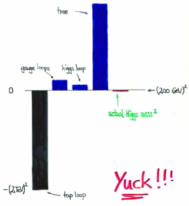
Figure 30: Contributions that must balance to great precision if the Higgs-boson mass is to take on a reasonable value, assuming that the electroweak theory is a good description of physics up to $10\hbox{ TeV}$ [45].

No principle forbids such a fine balance, but—as Martin Schmaltz’s editorial comment on his figure eloquently conveys—we have come to believe that Nature finds solutions more elegant than this one.

The supersymmetric solution does have the virtue of elegance [46, 47, 48, 49]. Exploiting the fact that fermion loops contribute with an overall minus sign (because of Fermi statistics), supersymmetry balances the contributions of fermion and boson loops. In the limit of unbroken supersymmetry, in which the masses of bosons are degenerate with those of their fermion counterparts, the cancellation is exact:

$$\sum_{{i={\rm fermions\atop+bosons}}}C_{i}\,g^{2}\!\!\!\int_{p^{2}}^{\Lambda^{2}}\!\!dk^{2}=0\;.$$ (4.1)

If the supersymmetry is broken (as it must be in our world), the contribution of the integrals may still be acceptably small if the fermion-boson mass splittings $\Delta M$ are not too large. The condition that $g^{2}\Delta M^{2}$ be “small enough” leads to the requirement that superpartner masses be less than about $1\hbox{ TeV}$.

In a recently constructed class of theories, called little Higgs models [50], the Higgs boson is interpreted as a pseudo-Nambu–Goldstone boson. A broken global symmetry arranges that the cancellation of the quantum corrections occurs between fields of the same spin: fermions cancel fermions and bosons cancel bosons. The models require new heavy fermionic partners for quarks and leptons, and also TeV-scale partners for gauge bosons [51, 52, 53].

A third solution to the problem of the enormous range of integration in (2.109) is offered by theories of dynamical symmetry breaking such as technicolor [54, 55]. In technicolor models, the Higgs boson is composite, and new physics arises on the scale of its binding, $\Lambda_{\mathrm{TC}}\simeq O(1~{}{\rm TeV})$. Thus the effective range of integration is cut off (effectively by form factor effects), and mass shifts are under control.

A fourth possibility is that the gauge sector becomes strongly interacting. This would give rise to $WW$ resonances, multiple production of gauge bosons, and other new phenomena at energies of 1 TeV or so. It is likely that a scalar bound state—a quasi-Higgs boson—would emerge with a mass less than about $1\hbox{ TeV}$ [56].

We cannot avoid the conclusion that some new physics must occur on the 1-TeV scale.

4.1 Supersymmetry

4.1.1 Why Supersymmetry?

Supersymmetry is a fermion–boson symmetry that arises from the presence of new fermionic dimensions. The most general symmetry of the $S$-matrix is Poincaré invariance plus internal symmetries—plus supersymmetry. The new symmetry relates fermion to boson degrees of freedom: roughly speaking, each particle has a superpartner with spin offset by $\cfrac{1}{2}$. The observed particle spectrum contains no fermion–boson mates that we can identify as superpartners. Accordingly, imposing supersymmetry requires doubling the spectrum of particles. The properties of the supersymmetric partners of the $\mathrm{SU(3)_{c}}\otimes\mathrm{SU(2)}_{\mathrm{L}}\otimes\mathrm{U(1)}_{Y}$ particles are shown in Table 2.

Table 2: Supersymmetric partners of $\mathrm{SU(3)_{c}}\otimes\mathrm{SU(2)}_{\mathrm{L}}\otimes\mathrm{U(1)}_{Y}$ fermions and gauge bosons.

Particle	Spin	Color	Charge	$R$-parity
$g$ gluon	1	8	0	$+1$
$\tilde{g}$  gluino	$\cfrac{1}{2}$	8	0	$-1$
$\gamma$  photon	1	1	0	$+1$
$\tilde{\gamma}$  photino	$\cfrac{1}{2}$	1	0	$-1$
$W^{\pm},\,Z^{0}$  intermediate bosons	1	1	$\pm 1,\,0$	$+1$
$\widetilde{W}^{\pm},\,\widetilde{Z}^{0}$  electroweak gauginos	$\cfrac{1}{2}$	1	$\pm 1,\,0$	$-1$
$q$  quark	$\cfrac{1}{2}$	3	$\cfrac{2}{3},\,-\cfrac{1}{3}$	$+1$
$\tilde{q}$  squark	$0$	3	$\cfrac{2}{3},\,-\cfrac{1}{3}$	$-1$
$\ell$  charged lepton	$\cfrac{1}{2}$	1	$-1$	$+1$
$\tilde{\ell}$  charged slepton	0	1	$-1$	$-1$
$\nu$  neutrino	$\cfrac{1}{2}$	1	$0$	$+1$
$\tilde{\nu}$  sneutrino	$0$	1	$0$	$-1$

In a supersymmetric theory, two Higgs doublets are required to give masses to fermions with weak isospin $I_{3}=\cfrac{1}{2}$ and $I_{3}=-\cfrac{1}{2}$. Let us designate the two doublets as $\Phi_{1}$ and $\Phi_{2}$. Before supersymmetry is broken, the scalar potential has the form

$$V=\mu^{2}(\Phi_{1}^{2}+\Phi_{2}^{2})+\frac{g^{2}+g^{\prime 2}}{8}(\Phi_{1}^{2}+\Phi_{2}^{2})^{2}+\frac{g^{2}}{2}\left|\Phi_{1}^{*}\cdot\Phi_{2}\right|^{2}\;.$$ (4.2)

By adding all possible soft supersymmetry-breaking terms, we raise the possibility that the electroweak symmetry will be broken. We choose

$$\begin{array}[]{c}\langle\Phi_{1}\rangle_{0}=v_{1}>0\;,\\[6.0pt] \langle\Phi_{2}\rangle_{0}=v_{2}>0\;,\end{array}$$ (4.3)

with $v_{1}^{2}+v_{2}^{2}=v^{2}$ and

$$\frac{v_{2}}{v_{1}}\equiv\tan\beta\;.$$ (4.4)

After the $W^{\pm}$ and $Z^{0}$ acquire masses, five spin-zero degrees of freedom remain as massive spin-zero particles: the lightest scalar $h^{0}$, a heavier neutral scalar $H^{0}$, two charged scalars $H^{\pm}$, and a neutral pseudoscalar $A^{0}$.

Supersymmetry also relates the interactions of the superpartners to those of the known particles. In addition to transcriptions of the usual interactions, supersymmetry admits new Yukawa terms,

$$\mathcal{L}_{\mathrm{SUSY-Yuk}}=\lambda_{ijk}L^{i}L^{j}E^{k}+\lambda^{\prime}_{ijk}L^{i}Q^{j}\bar{D}^{k}+\lambda^{\prime\prime}\bar{U}^{i}\bar{D}^{j}\bar{D}^{k}\;,$$ (4.5)

that entail 45 new free parameters. The new interactions in (4.5) induce dangerous lepton- and baryon-number violations. For example, expanding the first term we have

$$\mathcal{L}_{LLE}=\lambda_{ijk}\,\tilde{\nu}^{i}_{L}e^{i}_{L}\bar{e}^{k}_{R}+\ldots$$ (4.6)

To banish these, it has become conventional to impose symmetry under $R$-parity,

$$R=(-1)^{3B+L+S},$$ (4.7)

a multplicative quantum number that is even for the known particles and odd for superpartners. In a theory that conserves $R$-parity, the superpartners must be produced in pairs and the lightest superpartner (LSP) is stable. A neutral LSP is a promising dark matter candidate [64].

An interesting feature of supersymmetric theories is the possibility that spontaneous electroweak symmetry might be driven by a heavy top quark, provided that $55\hbox{ GeV}\mathop{\raisebox{-1.72218pt}{\hbox to0.0pt{$\sim$\hss}}\raisebox{1.72218pt}{$<$}}m_{t}\mathop{\raisebox{-1.72218pt}{\hbox to0.0pt{$\sim$\hss}}\raisebox{1.72218pt}{$<$}}200\hbox{ GeV}$. In a supersymmetric unified theory, the large top-quark Yukawa coupling drives the mass-squared of the Higgs boson responsible for $I_{3}=\cfrac{1}{2}$ masses to negative values at low energies [65, 66], as shown in Figure 31 for a 175-GeV top quark.

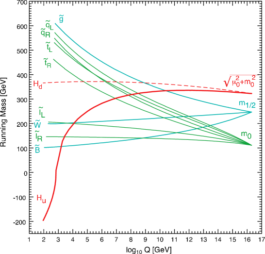
Figure 31: Evolution of superpartner masses in constrained minimal supersymmetry, from Ref. [67]. The sign of $M^{2}$ is indicated.

The resulting Higgs potential is minimized with a nonzero vacuum expectation value for the Higgs field—corresponding to hidden electroweak symmetry.

One of the best phenomenological motivations for supersymmetry on the 1-TeV scale is that the minimal supersymmetric extension of the standard model so closely approximates the standard model itself. A nice illustration of the small differences between predictions of supersymmetric models and the standard model is the compilation of pulls prepared by Erler and Pierce [68], which is shown in Figure 32.

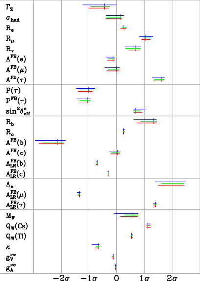
Figure 32: The range of best fit predictions of precision observables in the supergravity model (upper horizontal lines), the $\mathbf{5}\oplus\mathbf{5^{*}}$ gauge-mediated model (middle lines), the $\mathbf{10}\oplus\mathbf{10^{*}}$ gauge-mediated model (lower lines), and in the standard model at its global best fit value (vertical lines), in units of standard deviation, from Ref. [68].

This is a nontrivial property of new physics beyond the standard model, and a requirement urged on us by the unbroken quantitative success of the established theory.

4.1.2 Coupling Constant Unification in Supersymmetric Unification

We found in §3.3 that in a unified theory of the strong, weak, and electromagnetic interactions based on the gauge symmetry $\mathrm{SU(5)}$, the couplings $1/\alpha_{1}$, $1/\alpha_{2}$, and $1/\alpha_{3}$ tend to approach each other at high energies, but fail to coincide at a single point we would identify as the unification energy $U$. The evolution of the couplings is changed appreciably by the influence of supersymmetry’s richer spectrum—gluinos, squarks, sleptons, the second Higgs doublet, gauginos, and Higgsinos. It would be an important indirect encouragement for the development of supersymmetric models to find that a supersymmetrized version of our example unified theory does unify the couplings, so let us check. Working again to leading logarithmic approximation, we have

$$\hbox{SUSY }\mathrm{SU(3)_{\mathrm{c}}:}\quad 1/\alpha_{3}(Q^{2})=1/\alpha_{3}(\mu^{2})+b_{3}\log(Q^{2}/\mu^{2})\;,$$ (4.8)

where $4\pi b_{3}=9-2n_{\mathrm{gen}}$, so that $b_{3}=3/4\pi$; in the normal $\mathrm{SU(5)}$ theory, it was $7/4\pi$ (3.9).

$$\hbox{SUSY }\mathrm{SU(2)_{\mathrm{L}}:}\quad 1/\alpha_{2}(Q^{2})=1/\alpha_{2}(\mu^{2})+b_{2}\log(Q^{2}/\mu^{2})\;,$$ (4.9)

where $4\pi b_{2}=6-2n_{\mathrm{gen}}-\cfrac{1}{2}n_{\mathrm{Higgs}}$, so that $b_{2}=-1/4\pi$; without supersymmetry, it was $19/24\pi$ (3.10).

$$\hbox{SUSY }\mathrm{U(1)}_{Y}:\quad 1/\alpha_{1}(Q^{2})=1/\alpha_{Y}(\mu^{2})+b_{1}\log(Q^{2}/\mu^{2})\;,$$ (4.10)

with $4\pi b_{1}=-2n_{\mathrm{gen}}-\cfrac{3}{10}n_{\mathrm{Higgs}}$, so that $b_{1}=-33/20\pi$; it had been $-41/40\pi$ (3.11). As usual, $Q^{2}$ is the scale of interest and $\mu^{2}$ is the reference scale.

Using the new evolution equations (4.8) – (4.10) all the way down to $M_{Z}^{2}$, since a supersymmetric solution to the hierarchy problem demands that superpartner masses are $\mathop{\raisebox{-1.72218pt}{\hbox to0.0pt{$\sim$\hss}}\raisebox{1.72218pt}{$<$}}1\hbox{ TeV}$, we estimate the unification scale $U_{\mathrm{SUSY}}\approx 4\times 10^{16}\hbox{ GeV}$ and the unified coupling $1/\alpha_{U_{\mathrm{SUSY}}}\approx 24.6$; in the pure $\mathrm{SU(5)}$ case, we found $U\approx 10^{15}\hbox{ GeV}$ and $1/\alpha_{U}\approx 42$. As before, we have taken as inputs $\alpha_{3}(M_{Z}^{2})\approx 1/8.75$, $\alpha(M_{Z}^{2})\approx 1/128.9$, and $M_{Z}\approx 91.19\hbox{ GeV}$. Now for the test: we evaluate the weak mixing parameter at the weak scale and find

$$\left.x_{W}(M_{Z}^{2})\right|_{\mathrm{SUSY~{}SU(5)}}\approx 0.23\;,$$ (4.11)

whereas $\mathrm{SU(5)}$ unification gave $0.21$ (3.18). The supersymmetric prediction, (4.11), is in very suggestive agreement with the measured value, $0.2314\pm 0.003$ (3.19).

To test coupling constant unification graphically, we set the superpartner threshold at $1\hbox{ TeV}$ and evolve the couplings from $M_{Z}^{2}$ up to a high scale. The results displayed in Figure 33

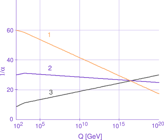
Figure 33: Running of $1/\alpha_{1},1/\alpha_{2},1/\alpha_{3}$ in the supersymmetric $\mathrm{SU(5)}$ unified theory, with the superpartner threshold at $1\hbox{ TeV}$.

show that the three values do indeed coincide in the neighborhood of $4\times 10^{16}\hbox{ GeV}$. This is a highly gratifying outcome for the hypothesis that supersymmetry operates on the electroweak scale.

4.1.3 The Lightest Higgs Boson

At tree level, we may express all the (pseudo)scalar masses in terms of $M_{A}$ and $\tan\beta$, to find

$$M_{h^{0},H^{0}}^{2}=\frac{1}{2}\left\{M_{A}^{2}+M_{Z}^{2}\mp\left[(M_{A}^{2}+M_{Z}^{2})^{2}-4M_{A}^{2}M_{Z}^{2}\cos^{2}2\beta\right]^{1/2}\right\}\;,$$ (4.12)

and

$$M_{H^{\pm}}^{2}=M_{W}^{2}+M_{A}^{2}\;.$$ (4.13)

At tree level, there is a simple mass hierarchy, given by

$$M_{h^{0}} < M_{Z}|\cos 2\beta|$$

$$M_{H^{0}} > M_{Z}$$ (4.14)

$$M_{H^{\pm}} > M_{W}\;,$$

but there are very important positive loop corrections to $M_{h^{0}}^{2}$ (proportional to $G_{\mathrm{F}}m_{t}^{4}$) that were neglected in the earliest calculations. These loop corrections change the mass predictions very significantly.

Because the minimal supersymmetric standard model (MSSM) implies upper bounds on the mass of the lightest scalar $h^{0}$, it sets attractive targets for experiment. Two such upper bounds are shown as functions of the top-quark mass in Figure 34.

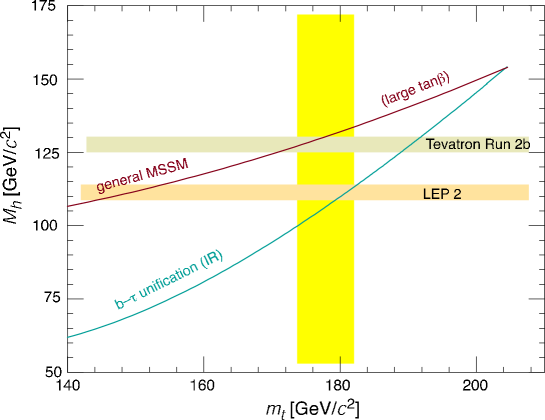
Figure 34: Upper bounds on the mass of the lightest Higgs boson, as a function of the top-quark mass, in two variants of the minimal supersymmetric standard model. The upper curve refers to a general MSSM, in the large-$\tan\beta$ limit; the lower curve corresponds to an infrared-fixed-point scenario with $b$-$\tau$ unification, from Ref. [70].

The large-$\tan\beta$ limit of a general MSSM yields the upper curve; an infrared-fixed-point scheme with $b$-$\tau$ unification produces an upper bound characterized by the lower curve. The vertical band shows the range $m_{t}=178.0\pm 4.3\hbox{ GeV}$ favored by Tevatron experiments [23]. The LEP 2 experiments [71, 29] have explored the full range of lightest-Higgs masses that occur in the infrared-fixed-point scheme. High-luminosity running at the Tevatron collider can extend the search field and, in the limit, explore much of the range of $h^{0}$ masses allowed in the MSSM [72, 73]. The ATLAS [74] and CMS experiments[75, 76] at the Large Hadron Collider will carry the Higgs-boson search up to $1\hbox{ TeV}$. A future electron-positron linear collider can carry out incisive studies of the lightest Higgs boson and of many superpartners [77].

4.1.4 The Stability of Matter

Supersymmetry doubles the spectrum of fundamental particles. We know that supersymmetry must be significantly broken in Nature, because the electron is manifestly not degenerate in mass with its scalar partner, the selectron. It is interesting to contemplate just how different the world would have been if the selectron, not the electron, were the lightest charged particle and therefore the stable basis of everyday matter [78]. If atoms were selectronic, there would be no Pauli principle to dictate the integrity of molecules. As Dyson [79] and Lieb [80] demonstrated, transforming electrons and nucleons from fermions to bosons would cause all molecules to shrink into an insatiable undifferentiated blob. Luckily, there is no analogue of chiral symmetry to guarantee naturally small squark and slepton masses. So while supersymmetry menaces us with an amorphous death, it is likely that a full understanding of supersymmetry will enable us to explain why we live in a universe ruled by the exclusion principle.

4.1.5 Challenges for Supersymmetry

Supersymmetry is an elegant idea, but if it applies to our world, supersymmetry is hidden. Some undiscovered dynamics will be required to explain supersymmetry breaking. The attractive notion of “soft” supersymmetry breaking leads us to the minimal supersymmetric standard model (MSSM), with 124 parameters—a large number to track, which doesn’t instantly present it as progress over the eighteen or so of the standard model.

Theorists have invented a number of crafty schemes for supersymmetry breaking. The best known is called gravity mediation, in which supersymmetry breaking at a very high scale is communicated to the standard model by gravitational interactions. In gauge mediation, supersymmetry breaking occurs relatively near to the electroweak scale, perhaps below $100\hbox{ TeV}$, and that is communicated to the standard model by possibly nonperturbative gauge forces. Other schemes provide more or less natural solutions to one or another requirement, but it is fair to say that none meets all the challenges.

Let us list some of the issues we shall have to face to construct a fully acceptable supersymmetric theory. $\Box$ Weak-scale supersymmetry (i.e., superpartners on the electroweak scale) protects the Higgs-boson mass and keeps it naturally below $1\hbox{ TeV}$, but does not explain the why the weak scale itself is so much smaller than the Planck scale. This is called the $\mu$ problem. $\Box$ Global supersymmetry must deal with the threat of flavor-changing neutral currents. $\Box$ In parallel with the standard model, supersymmetric models make reasonably clear predictions for the masses of gauge bosons and gauge fermions (gauginos), but are more equivocal about the masses of squarks and sleptons. $\Box$ Not only is supersymmetry a hidden symmetry in the technical sense, it seems to be a very well hidden symmetry, in that we have no direct experimental evidence in its favor. A certain number of contortions are required to accommodate a (lightest) Higgs-boson mass above $115\hbox{ GeV}$. $\Box$ We might have hoped that supersymmetry would relate particles to forces—quarks and leptons to gauge bosons—but instead it doubled the spectrum. $\Box$ Dangerous baryon- and lepton-number–violating interactions arise naturally from a supersymmetric Lagrangian, but we have only learned to banish them by decree. $\Box$ Supersymmetry introduces new sources of $\mathcal{CP}$ violation that are potentially too large. $\Box$ We haven’t yet found a convincing and viable picture of the TeV superworld.

This long list of challenges does not mean that supersymmetry is wrong, or even that it is irrelevant to the 1-TeV scale. But SUSY is not automatically right, either! If supersymmetry does operate on the 1-TeV scale, then Nature must have found solutions to all these challenges …and we will need to find them, too. The discovery of supersymmetry will mark a beginning, not an end, of our learning.

If supersymmetry is the solution to electroweak symmetry breaking and the hierarchy problem, then we should see concrete evidence of it soon, in the Higgs sector and beyond. The thicket of thresholds to be explored in electron-positron annihilations into pairs of superpartners shown in Figure 35 indicates that

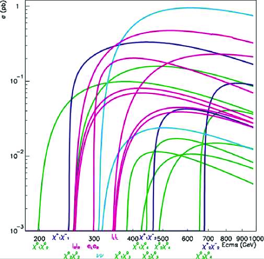
Figure 35: Cross sections for electron-positron annihilations to pairs of superpartners in a minimal supergravity model, with $\tan\beta=3$ (Grahame Blair, unpublished).

if weak-scale supersymmetry is real, we shall live in “interesting times.”

In my view, supersymmetry is (almost) certain to be true, as a path to the incorporation of gravity. Whether supersymmetry resolves the problems of the 1-TeV scale is a logically separate question, to which the answer is less obvious. Experiment will decide!

4.2 Electroweak Symmetry Breaking: Another Path?

Dynamical symmetry breaking offers a different solution to the naturalness problem of the electroweak theory: in technicolor, there are no elementary scalars. We hope that solving the dynamics that binds elementary fermions into a composite Higgs boson and other $WW$ resonances will bring addition predictive power. It is worth saying that technicolor is a far more ambitious program than global supersymmetry. It doesn’t merely seek to finesse the hierarchy problem, it aims to predict the mass of the Higgs surrogate. Against the aesthetic appeal of supersymmetry we can weigh technicolor’s excellent pedigree. As we have seen in §2.3, the Higgs mechanism of the standard model is the relativistic generalization of the Ginzburg-Landau description of the superconducting phase transition. Dynamical symmetry breaking schemes—technicolor and its relatives—are inspired by the Bardeen–Cooper–Schrieffer theory of superconductivity, and seek to give a similar microscopic description of electroweak symmetry breaking.

The dynamical-symmetry-breaking approach realized in technicolor theories is modeled upon our understanding of the superconducting phase transition. The macroscopic order parameter of the Ginzburg-Landau phenomenology corresponds to the wave function of superconducting charge carriers, which acquires a nonzero vacuum expectation value in the superconducting state. The microscopic Bardeen-Cooper-Schrieffer theory [81] identifies the dynamical origin of the order parameter with the formation of bound states of elementary fermions, the Cooper pairs of electrons. The basic idea of technicolor is to replace the elementary Higgs boson with a fermion-antifermion bound state. By analogy with the superconducting phase transition, the dynamics of the fundamental technicolor gauge interactions among technifermions generate scalar bound states, and these play the role of the Higgs fields.

The elementary fermions—electrons—and gauge interactions—QED—needed to generate the scalar bound states are already present in the case of superconductivity. Could a scheme of similar economy account for the transition that hides the electroweak symmetry? Consider an $\mathrm{SU(3)_{c}}\otimes\mathrm{SU(2)}_{\mathrm{L}}\otimes\mathrm{U(1)}_{Y}$ theory of massless up and down quarks. Because the strong interaction is strong, and the electroweak interaction is feeble, we may treat the $\mathrm{SU(2)}_{\mathrm{L}}\otimes\mathrm{U(1)}_{Y}$ interaction as a perturbation. For vanishing quark masses, QCD has an exact $\mathrm{SU(2)_{L}\otimes SU(2)_{R}}$ chiral symmetry. At an energy scale $\sim\Lambda_{\mathrm{QCD}},$ the strong interactions become strong, fermion condensates appear, and the chiral symmetry is spontaneously broken to the familiar flavor symmetry:

$$\mathrm{SU(2)_{L}\otimes SU(2)_{R}\to SU(2)_{V}}\;\;.$$ (4.15)

Three Goldstone bosons appear, one for each broken generator of the original chiral invariance. These were identified by Nambu [82] as three massless pions.

The broken generators are three axial currents whose couplings to pions are measured by the pion decay constant $f_{\pi}$. When we turn on the $\mathrm{SU(2)}_{\mathrm{L}}\otimes\mathrm{U(1)}_{Y}$ electroweak interaction, the electroweak gauge bosons couple to the axial currents and acquire masses of order $\sim gf_{\pi}$. The mass-squared matrix,

$$\mathcal{M}^{2}=\left(\begin{array}[]{cccc}g^{2}&0&0&0\\ 0&g^{2}&0&0\\ 0&0&g^{2}&gg^{\prime}\\ 0&0&gg^{\prime}&g^{\prime 2}\end{array}\right)\frac{f_{\pi}^{2}}{4}\;,$$ (4.16)

(where the rows and columns correspond to $W^{+}$, $W^{-}$, $W_{3}$, and $\mathcal{A}$) has the same structure as the mass-squared matrix for gauge bosons in the standard electroweak theory. Diagonalizing the matrix (4.16), we find that $M_{W}^{2}=g^{2}f_{\pi}^{2}/4$ and $M_{Z}^{2}=(g^{2}+g^{\prime 2})f_{\pi}^{2}/4$, so that

$$\frac{M_{Z}^{2}}{M_{W}^{2}}=\frac{(g^{2}+g^{\prime 2})}{g^{2}}=\frac{1}{\cos^{2}\theta_{W}}\;.$$ (4.17)

The photon emerges massless.

The massless pions thus disappear from the physical spectrum, having become the longitudinal components of the weak gauge bosons. Unfortunately, the mass acquired by the intermediate bosons is far smaller than required for a successful low-energy phenomenology; it is only [57] $M_{W}\approx 30\hbox{ MeV}\!/\!c^{2}$.

The minimal technicolor model of Weinberg [83] and Susskind [84] transcribes the same ideas from QCD to a new setting. The technicolor gauge group is taken to be $\mathrm{SU}(N)_{\mathrm{TC}}$ (usually $\mathrm{SU(4)}_{\mathrm{TC}}$), so the gauge interactions of the theory are generated by

$$\mathrm{SU(4)_{\mathrm{TC}}\otimes SU(3)_{c}\otimes SU(2)_{L}\otimes U(1)_{\mathit{Y}}}\;.$$ (4.18)

The technifermions are a chiral doublet of massless color singlets

$$\begin{array}[]{cc}\left(\begin{array}[]{c}U\\ D\end{array}\right)_{\mathrm{L}}&U_{\mathrm{R}},\;D_{\mathrm{R}}\;.\end{array}$$ (4.19)

With the electric charge assignments $Q(U)=\frac{1}{2}$ and $Q(D)=-\frac{1}{2}$, the theory is free of electroweak anomalies. The ordinary fermions are all technicolor singlets.

In analogy with our discussion of chiral symmetry breaking in QCD, we assume that the chiral TC symmetry is broken,

$$\mathrm{SU(2)_{L}\otimes SU(2)_{R}\otimes U(1)_{V}\to SU(2)_{V}\otimes U(1)_{V}}\;.$$ (4.20)

Three would-be Goldstone bosons emerge. These are the technipions

$$\begin{array}[]{ccc}\pi_{T}^{+},&\pi_{T}^{0},&\pi_{T}^{-},\end{array}$$ (4.21)

for which we are free to choose the technipion decay constant as

$$F_{\pi}=\left(G_{\mathrm{F}}\sqrt{2}\right)^{-1/2}=246\hbox{ GeV}\;.$$ (4.22)

This amounts to choosing the scale on which technicolor becomes strong. When the electroweak interactions are turned on, the technipions become the longitudinal components of the intermediate bosons, which acquire masses

$$\begin{array}[]{ccccc}M_{W}^{2}&=&g^{2}F_{\pi}^{2}/4&=&{\displaystyle\frac{\pi\alpha}{G_{\mathrm{F}}\sqrt{2}\sin^{2}\theta_{W}}}\\ M_{Z}^{2}&=&\left(g^{2}+g^{\prime 2}\right)F_{\pi}^{2}/4&=&M_{W}^{2}/\cos^{2}\theta_{W}\end{array}\;,$$ (4.23)

that have the canonical standard model values, thanks to our choice (4.22) of the technipion decay constant.

Technicolor shows how the generation of intermediate boson masses could arise without fundamental scalars or unnatural adjustments of parameters. It thus provides an elegant solution to the naturalness problem of the standard model. However, it has a major deficiency: it offers no explanation for the origin of quark and lepton masses, because no Yukawa couplings are generated between Higgs fields and quarks or leptons. Consequently, technicolor serves as a reminder that there are two problems of mass: explaining the masses of the gauge bosons, which demands an understanding of electroweak symmetry breaking; and accounting for the quark and lepton masses, which requires not only an understanding of electroweak symmetry breaking but also a theory of the Yukawa couplings that set the scale of fermion masses in the standard model. We can be confident that the origin of gauge-boson masses will be understood on the 1-TeV scale. We do not know where we will decode the pattern of the Yukawa couplings; we looked at one approach in § 3.4.

To generate fermion mass, we may embed technicolor in a larger extended technicolor gauge group $G_{\mathrm{ETC}}\supset G_{\mathrm{TC}}$ that couples the quarks and leptons to technifermions [85, 86]. If the $G_{\mathrm{ETC}}$ gauge symmetry is broken down to $G_{\mathrm{TC}}$ at a scale $\Lambda_{\mathrm{ETC}}$, then the quarks and leptons can acquire masses

$$m\sim\frac{g_{\mathrm{ETC}}^{2}F_{\pi}^{3}}{\Lambda_{\mathrm{ETC}}^{2}}\;,$$ (4.24)

through the “radiative” mechanism shown in Figure 36.

Figure 36: In extended technicolor, mass is conveyed to the quarks and leptons through the interaction of ETC gauge bosons with the TC condensate.

There is no standard technicolor model, in large measure because the straightforward implementations of extended technicolor are challenged to reproduce the wide range of quark masses while avoiding flavor-changing-neutral-current traps. Consider $\left|\Delta S\right|=2$ interactions,

$${\mathcal{L}_{\left|\Delta S\right|=2}=\frac{g_{\mathrm{ETC}}^{2}\theta_{sd}^{2}}{M_{\mathrm{ETC}}^{2}}(\bar{s}\Gamma^{\mu}d)(\bar{s}\Gamma^{\prime}_{\mu}d)+\cdots}$$ (4.25)

The tiny $K_{\mathrm{L}}$-$K_{\mathrm{S}}$ mass difference, $\Delta M_{K}<3.5\times 10^{-12}\hbox{ MeV}$, implies that ${{M_{\mathrm{ETC}}^{2}}/{g_{\mathrm{ETC}}^{2}\left|\theta_{sd}\right|^{2}}}$ must be very great, but that makes it hard to generate large enough masses for $c$, $s$, $t$, $b$. Multiscale technicolor [87] is a possible approach; it entails many fermions in different technicolor representations, which implies many technipions, among them light $\rho_{\mathrm{T}}$, $\omega_{\mathrm{T}}$, $\pi_{\mathrm{T}}$.

The generation of fermion mass is where all the experimental threats to technicolor arise. The rich particle content of ETC models generically leads to quantum corrections that are in conflict with precision electroweak measurements.  Moreover, if quantum chromodynamics is a good model for the chiral-symmetry breaking of technicolor, then extended technicolor produces flavor-changing neutral currents at uncomfortably large levels. We conclude that QCD must not provide a good template for the technicolor interaction. Keep in mind that, in addressing the origins of fermion mass, extended technicolor is much more ambitious than many implementations of global supersymmetry. For the current state of model building, see the lectures by Lane [54] and the comprehensive review article by Hill and Simmons [55].

4.3 Why is the Planck scale so large?

Our understanding of gravity has been handed down to us by Newton and Einstein and the gods, whereas the electroweak theory is the work of mortals of our own time. It is therefore not surprising that the conventional approach to new physics has been to extend the standard model to understand why the electroweak scale (and the mass of the Higgs boson) is so much smaller than the Planck scale. A novel approach, only a few years old, is instead to change gravity to understand why the Planck scale is so much greater than the electroweak scale [90, 91, 92]. Now, experiment tells us that gravitation closely follows the Newtonian force law down to distances on the order of $1\hbox{ mm}$. Let us parameterize deviations from a $1/r$ gravitational potential in terms of a relative strength $\varepsilon_{\mathrm{G}}$ and a range $\lambda_{\mathrm{G}}$, so that

$$V(r)=-\int dr_{1}\int dr_{2}\frac{G_{\mathrm{Newton}}\rho(r_{1})\rho(r_{2})}{r_{12}}\left[1+\varepsilon_{\mathrm{G}}\exp(-r_{12}/\lambda_{\mathrm{G}})\right]\;,$$ (4.26)

where $\rho(r_{i})$ is the mass density of object $i$ and $r_{12}$ is the separation between bodies 1 and 2. Elegant experiments [93] using torsion oscillators and microcantilevers imply bounds on anomalous gravitational interactions, as shown in Figure 37. Below about a millimeter, the

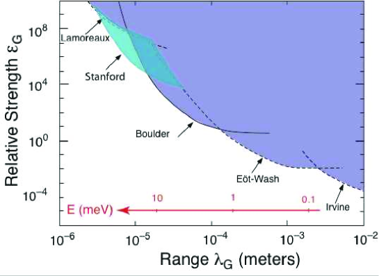
Figure 37: 95% confidence level upper limits on the strength $\varepsilon_{\mathrm{G}}$ (relative to gravity) versus the range $\lambda_{\mathrm{G}}$ of a new long-range force characterized by (4.26), from recent experiments at Boulder [94], Stanford [95], and Washington [96]. The region excluded by earlier work[97, 98, 99] lies above the heavy lines labeled Irvine, Moscow and Lamoreaux, respectively. The red scale running from right to left shows the corresponding energy, $E=(\hbar c/\lambda_{\mathrm{G}})$.

constraints on deviations from Newton’s inverse-square force law deteriorate rapidly, so nothing prevents us from considering changes to gravity even on a small but macroscopic scale. Even after this new generation of experiments, we have only tested our understanding of gravity—through the inverse-square law—up to energies of 10 meV (yes, milli-electron volts), some fourteen orders of magnitude below the energies at which we have studied QCD and the electroweak theory. Experiment plainly leaves an opening for gravitational surprises.

For its internal consistency, string theory requires an additional six or seven space dimensions, beyond the $3+1$ dimensions of everyday experience [100]. Until recently it has been presumed that the extra dimensions must be compactified on the Planck scale, with a compactification radius $R_{\mathrm{unobserved}}\approx 1/M_{\mathrm{Planck}}\approx 1.6\times 10^{-35}\hbox{ m}$. One new wrinkle is to consider that the $\mathrm{SU(3)_{c}}\otimes\mathrm{SU(2)}_{\mathrm{L}}\otimes\mathrm{U(1)}_{Y}$ standard-model gauge fields, plus needed extensions, reside on $3+1$-dimensional branes, not in the extra dimensions, but that gravity can propagate into the extra dimensions.

How does this hypothesis change the picture? The dimensional analysis (Gauss’s law, if you like) that relates Newton’s constant to the Planck scale changes. If gravity propagates in $n$ extra dimensions with radius $R$, then

$$G_{\mathrm{Newton}}\sim M_{\mathrm{Planck}}^{-2}\sim M^{\star\,-n-2}R^{-n}\;,$$ (4.27)

where $M^{\star}$ is gravity’s true scale. Notice that if we boldly take $M^{\star}$ to be as small as $1\hbox{ TeV}$, then the radius of the extra dimensions is required to be smaller than about $1\hbox{ mm}$, for $n\geq 2$. If we use the four-dimensional force law to extrapolate the strength of gravity from low energies to high, we find that gravity becomes as strong as the other forces on the Planck scale, as shown by the dashed line in Figure 38. If the force law changes at an energy $1/R$, as the large-extra-dimensions scenario suggests, then the forces are unified at an energy $M^{\star}$, as shown by the solid line in Figure 38. What we know as the Planck scale is then a mirage that results from a false extrapolation: treating gravity as four-dimensional down to arbitrarily small distances, when in fact—or at least in this particular fiction—gravity propagates in $3+n$ spatial dimensions. The Planck mass is an artifact, given by $M_{\mathrm{Planck}}=M^{\star}(M^{\star}R)^{n/2}$.

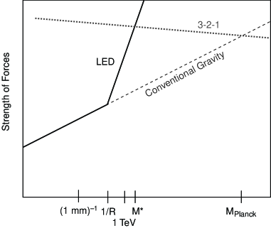
Figure 38: One of these extrapolations (at least!) is false.

Although the idea that extra dimensions are just around the corner—either on the submillimeter scale or on the TeV scale—is preposterous, it is not ruled out by observations. For that reason alone, we should entertain ourselves by entertaining the consequences. Many authors have considered the gravitational excitation of a tower of Kałuza–Klein modes in the extra dimensions, which would give rise to a missing (transverse) energy signature in collider experiments [101].

The electroweak scale is nearby; indeed, it is coming within experimental reach at the Tevatron Collider and the Large Hadron Collider. Where are the other scales of significance? In particular, what is the energy scale on which the properties of quark and lepton masses and mixings are set? The similarity between the top-quark mass, $m_{t}\approx 175\hbox{ GeV}$, and the Higgs-field vacuum expectation value, $v/\sqrt{2}\approx 174\hbox{ GeV}$, encourages the hope that in addition to decoding the puzzle of electroweak symmetry breaking in our explorations of the 1-TeV scale, we might gain insight into the problem of fermion mass. This is an area to be defined over the next decade.

4.4 New Departures

In the time available to us in San Miguel Regla, it hasn’t been possible to examine all the promising attempts to complete the electroweak theory. Over the past five years, many stimulating ideas have been inspired by the notion that our spacetime is larger than four-dimensional. In many ways, the theoretical imagination has been liberated, and we have seen many proposals that—whatever their eventual fate—have been mind-expanding, showing us ways to think about problems that we had not known before.

Randall and Sundrum [102] proposed a higher-dimensional solution to the hierarchy problem that uses one warped extra dimension to generate the weak scale from the Planck scale by means of the background metric. The simplest example entails two three-branes, one of which contains the standard-model fields. Other groups, including [103], have now explored the idea that the Higgs boson might be regarded as an extra-dimensional component of a gauge boson. A related approach, which takes the Higgs boson as a pseudo-Goldstone boson, gives rise to the “little Higgs” models [104] mentioned in passing at the beginning of § 4 Universal extra dimensions at a compactification scale as low as a few hundred GeV survive current experimental constraints [105], and might be discovered at the Tevatron collider. Supersymmetry and dynamical symmetry breaking may be combined; a recent example is the so-called “fat Higgs” model [106] to solve supersymmetry’s little hierarchy problem: constraints from precision electroweak measurements reveal no evidence for new physics up to about $5\hbox{ TeV}$, but if supersymmetry stabilizes the Higgs-boson mass, superpartner masses should be no more than about $1\hbox{ TeV}$. Another suggestion [107] is that Kałuza–Klein (extra-dimensional) excitations of gauge fields could take the place of a Higgs scalar, at least in the framework of an effective field theory at low energies. An extra-dimensional generation of the QCD (chiral-symmetry-breaking) mechanism we discussed in § 4.2 might be all that is required to hide the electroweak symmetry through a top-quark seesaw [108].

This incomplete list indicates the vitality of theoretical speculation about the mechanism for electroweak symmetry breaking and underscores the urgency of a thorough exploration of the 1-TeV scale. We have much, much more to accomplish than to find one particle!

Before summing up, let us consider another round of questions that have come to our attention:

Fourth Harvest of Questions

• Why is the world built of fermions, not bosons—i.e., quarks not squarks, leptons not sleptons?

• Does gravity follow Newton’s force law to very large distances? … to very short distances?

• Why is gravity weak?

• Is $\mathcal{CPT}$ a good symmetry?

• Is Lorentz invariance exact?

• Are there extra dimensions?

• Is local field theory the ultimate framework?

• Can causality be violated?

• What is dark matter?

• What drives inflation?

• What is the origin of dark energy?

5 Outlook

In the midst of a revolution in our conception of Nature, we confront many fundamental questions about our world of diversity and change. I find it instructive to organize our concerns around a small number of broad themes.

Elementarity. Are the quarks and leptons structureless, or will we find that they are composite particles with internal structures that help us understand the properties of the individual quarks and leptons? If the quarks and leptons do have internal structure, of what are they made? What is the compositeness scale, and how does it relate to other important scales?

Symmetry. One of the most powerful lessons of the modern synthesis of particle physics is that (local) symmetries prescribe interactions. Our investigation of symmetry must address the question of which gauge symmetries exist (and, eventually, why). Will we find additional fundamental forces, reflecting new symmetries? We have learned to seek symmetry in the laws of Nature, not (necessarily) in the consequences of those laws. Accordingly, we must understand how the symmetries are hidden from us in the world we inhabit. For the moment, the most urgent problem in particle physics is to complete our understanding of electroweak symmetry breaking by exploring the 1-TeV scale. This is the business of the experiments at the Tevatron Collider, the Large Hadron Collider, and an $e^{+}e^{-}$ linear collider.

Unity. In the sense of developing explanations that apply not to one individual phenomenon in isolation, but to many phenomena in common, unity is central to all of physics, and indeed to all of science. At this moment in particle physics, our quest for unity takes several forms. $\Box$ First, we have the fascinating possibility of gauge coupling unification, the idea that all the interactions we encounter have a common origin and thus a common strength at suitably high energy. $\Box$ Second, there is the imperative of anomaly freedom in the electroweak theory, which urges us to treat quarks and leptons together, not as completely independent species. Both of these ideas are embodied, of course, in unified theories of the strong, weak, and electromagnetic interactions, which imply the existence of still other forces—to complete the grander gauge group of the unified theory—including interactions that change quarks into leptons. $\Box$ The third aspect of unity is the idea that the traditional distinction between force particles and constituents might give way to a unified understanding of all the particles. The gluons of QCD carry color charge, so we can imagine quarkless hadronic matter in the form of glueballs. Beyond that breach in the wall between messengers and constituents, supersymmetry relates fermions and bosons. $\Box$ Finally, we desire a reconciliation between the pervasive outsider, gravity, and the forces that prevail in the quantum world of our everyday laboratory experience.

Identity. We do not understand the physics that sets quark masses and mixings. Although we are testing the idea that the phase in the quark-mixing matrix lies behind the observed $\mathcal{CP}$ violation, we do not know what determines that phase. The accumulating evidence for neutrino oscillations presents us with a new embodiment of these puzzles in the lepton sector. At bottom, the question of identity is very simple to state: What makes an electron and electron, and a top quark a top quark? Will we find new forms of matter, like the superpartners suggested by supersymmetry?

Topography. “What is the dimensionality of spacetime?” tests our preconceptions and unspoken assumptions. It is given immediacy by recent theoretical work. For its internal consistency, string theory requires an additional six or seven space dimensions, beyond the $3+1$ dimensions of everyday experience. Until recently it has been presumed that the extra dimensions must be compactified on the Planck scale, with a stupendously small compactification radius $R\simeq M_{\mathrm{Planck}}^{-1}=1.6\times 10^{-35}\hbox{ m}$. Part of the vision of string theory is that what goes on in even such tiny curled-up dimensions does affect the everyday world: excitations of the Calabi–Yau manifolds determine the fermion spectrum. We have recognized recently that Planck-scale compactification is not—according to what we can establish—obligatory, and that current experiment and observation admit the possibility of dimensions not navigated by the strong, weak, and electromagnetic interactions that are almost palpably large. A whole range of new experiments will help us explore the fabric of space and time, in ways we didn’t expect just a few years ago [110].

I hope that in the course of these lectures you have been prompted to ask yourselves many questions, and that you have enjoyed finding at least the beginning of “a lifetime of homework.” Many of the questions we have come upon together qualify as great questions. In the usual way of science, answering questions great and small can lead us toward the answers to yet broader and more cosmic questions. I believe that we are on the threshold of a remarkable flowering of experimental particle physics, and of theoretical physics that engages with experiment. We can be quite confident, I think, that the way we think about the laws of nature will be very different in ten or fifteen years from the conception we hold today. Over the next decade or two, we may hope to

Understand electroweak symmetry breaking Observe the Higgs boson Measure neutrino masses and mixings Establish Majorana neutrinos ($\beta\beta_{0\nu}$) Thoroughly explore CP violation in $B$ decays Exploit rare decays ($K$, $D$, …) Observe neutron EDM, pursue electron EDM Use top as a tool Observe new phases of matter Understand hadron structure quantitatively Uncover QCD’s full implications Observe proton decay Understand the baryon excess Catalogue matter and energy of the universe Measure dark energy equation of state Search for new macroscopic forces Determine GUT symmetry

Detect neutrinos from the universe Learn how to quantize gravity Learn why empty space is nearly weightless Test the inflation hypothesis Understand discrete symmetry violation Resolve the hierarchy problem Discover new gauge forces Directly detect dark-matter particles Explore extra spatial dimensions Understand the origin of large-scale structure Observe gravitational radiation Solve the strong CP problem Learn whether supersymmetry is TeV-scale Seek TeV-scale dynamical symmetry breaking Search for new strong dynamics Explain the highest-energy cosmic rays Formulate problem of identity

M …and learn the right questions to ask.

References

- [1] M. Gallinaro (CDF) (2003), hep-ph/0304211.
- [2] K. Hagiwara et al. (Particle Data Group), Physical Review D 66, 010001 (2002), and 2003 off-year partial update, pdg.lbl.gov.
- [3] C. S. Wu, E. Ambler, R. W. Hayward, D. D. Hoppes, and R. P. Hudson, Phys. Rev. 105, 1413 (1957).
- [4] R. A. Lyttleton and H. Bondi, Proc. Roy. Soc. London A252, 313 (1959).
- [5] J. C. Pati and A. Salam, Phys. Rev. D10, 275 (1974).
- [6] C. Quigg (2002), in Flavor Physics for the Millennium: TASI 2000, edited by Jonathan L. Rosner (World Scientific, Singapore, 2001), pp. 3 - 67, hep-ph/0204104.
- [7] V. L. Ginzburg and L. D. Landau, Zh. Eksp. Teor. Fiz. 20, 1064 (1950), English translation: Men of Physics: Landau, Vol. I, edited by D. ter Haar (Pergamon, New York, 1965), p. 138.
- [8] C. Quigg, Gauge Theories of the Strong, Weak, and Electromagnetic Interactions (Addison–Wesley, Reading, Mass., 1983).
- [9] P. W. Higgs, Phys. Lett. 12, 132 (1964), The parallel between electroweak symmetry breaking and the Ginzburg-Landau theory is drawn carefully in R. E. Marshak, Conceptual Foundations of Modern Particle Physics (World Scientific, Singapore, 1993), §4.4. For a rich discussion of superconductivity as a consequence of spontaneously broken electromagnetic gauge symmetry, see S. Weinberg, The Quantum Theory of Fields, vol. 2 (Cambridge University Press, Cambridge, 1996), §21.6.
- [10] F. J. Hasert et al. (Gargamelle Neutrino), Phys. Lett. B46, 138 (1973).
- [11] A. R. Barker (2000), in Flavor Physics for the Millennium: TASI 2000, edited by Jonathan L. Rosner (World Scientific, Singapore, 2001), pp. 209-240.
- [12] G. Buchalla (2001), in Flavor Physics for the Millennium: TASI 2000, edited by Jonathan L. Rosner (World Scientific, Singapore, 2001), pp. 143-205, hep-ph/0103166.
- [13] S. Adler et al. (E787) (2004), hep-ex/0403034.
- [14] A. V. Artamonov (E949) (2004), hep-ex/0403036.
- [15] D. Ambrose et al. (E871), Phys. Rev. Lett. 84, 1389 (2000).
- [16] S. L. Glashow, J. Iliopoulos, and L. Maiani, Phys. Rev. D2, 1285 (1970).
- [17] M. Kobayashi and T. Maskawa, Prog. Theor. Phys. 49, 652 (1973).
- [18] M. L. Swartz, Int. J. Mod. Phys. A15S1, 307 (2000), in Proc. of the 19th Intl. Symp. on Photon and Lepton Interactions at High Energy LP99 ed. J.A. Jaros and M.E. Peskin, [eConf C990809, 307 (2000)], hep-ex/9912026; see also A. Sirlin, Ibid. p. 398, hep-ph/9912227.
- [19] G. Altarelli and M. W. Grunewald (2004), hep-ph/0404165.
- [20] LEP Electroweak Working Group, www.cern.ch/LEPEWWG/.
- [21] ALEPH, http://aleph.web.cern.ch/aleph/aleph_general/reports/figures/ew/zline_aleph.gif, based on 1993 LEP data.
- [22] C. Quigg, Phys. Today 50, 20 (May 1997), hep-ph/9704332.
- [23] The Tevatron Electroweak Working Group (2004), hep-ex/0404010.
- [24] A. D. Linde, JETP Lett. 19, 183 (1974), Pisma Zh. Eksp. Teor. Fiz. 19, 320 (1974).
- [25] M. J. G. Veltman, Phys. Rev. Lett. 34, 777 (1975).
- [26] S. M. Carroll, ECONF C0307282, TTH09 (2003), astro-ph/0310342.
- [27] D. E. Groom et al. (Particle Data Group), Eur. Phys. J. C15, 1 (2000).
- [28] A. Lewis and S. Bridle, Phys. Rev. D66, 103511 (2002), astro-ph/0205436.
- [29] R. Barate et al. (ALEPH, DELPHI, L3, OPAL), Phys. Lett. B565, 61 (2003), hep-ex/0306033.
- [30] B. W. Lee, C. Quigg, and H. B. Thacker, Phys. Rev. D16, 1519 (1977).
- [31] J. M. Cornwall, D. N. Levin, and G. Tiktopoulos, Phys. Rev. D10, 1145 (1974), erratum—ibid. D11, 972 (1975).
- [32] M. S. Chanowitz and M. K. Gaillard, Nucl. Phys. B261, 379 (1985).
- [33] A. D. Linde, JETP Lett. 23, 64 (1976), Zh. Eksp. Teor. Fiz. Pis’ma Red. 23, 73 (1976).
- [34] S. Weinberg, Phys. Rev. Lett. 36, 294 (1976a).
- [35] P. Q. Hung, Phys. Rev. Lett. 42, 873 (1979).
- [36] G. Altarelli and G. Isidori, Phys. Lett. B337, 141 (1994).
- [37] J. R. Espinosa and M. Quirós, Phys. Lett. B353, 257 (1995), hep-ph/9504241.
- [38] M. J. G. Veltman, Acta Phys. Polon. B12, 437 (1981).
- [39] C. H. Llewellyn Smith, Phys. Rept. 105, 53 (1984).
- [40] C. G. Wohl (2002), in [2], pdg.lbl.gov/2002/youngrpp.pdf.
- [41] T. Affolder et al. (CDF), Phys. Rev. Lett. 88, 042001 (2002), hep-ex/0108034.
- [42] A. J. Buras, J. R. Ellis, M. K. Gaillard, and D. V. Nanopoulos, Nucl. Phys. B135, 66 (1978).
- [43] M.-C. Chen and K. T. Mahanthappa, Int. J. Mod. Phys. A18, 5819 (2003), hep-ph/0305088.
- [44] S. R. Elliott and P. Vogel, Ann. Rev. Nucl. Part. Sci. 52, 115 (2002), hep-ph/0202264.
- [45] M. Schmaltz, Nucl. Phys. Proc. Suppl. 117, 40 (2003), hep-ph/0210415.
- [46] J. D. Lykken (1996a), in Fields, Strings, and Duality: TASI 96, edited by C. Efthimiou and B. Greene (World Scientific, Singapore, 1997). p. 85, hep-th/9612114.
- [47] S. P. Martin (1997), “A Supersymmetry Primer,” in Perspectives on Supersymmetry, edited by G. L. Kane (World Scientific, Singapore, 1998), p. 1; the latest version is available at zippy.physics.niu.edu/primer.shtml, hep-ph/9709356.
- [48] S. Dawson (1997), in Supersymmetry, Supergravity and Supercolliders: TASI 97, edited by J. Bagger (World Scientific, Singapore, 1999), p. 261, hep-ph/9712464.
- [49] H. Murayama (2000), in Flavor Physics for the Millennium: TASI 2000, edited by Jonathan L. Rosner (World Scientific, Singapore, 2001), pp. 653-727.
- [50] M. Schmaltz, Phys. World 15, 23 (November 2002), physicsweb.org/article/world/15/11/3.
- [51] G. Burdman, M. Perelstein, and A. Pierce, Phys. Rev. Lett. 90, 241802 (2003), erratum—ibid. 92, 049903 (2004), hep-ph/0212228.
- [52] T. Han, H. E. Logan, B. McElrath, and L.-T. Wang, Phys. Rev. D67, 095004 (2003), hep-ph/0301040.
- [53] G. Azuelos et al. (2004), hep-ph/0402037.
- [54] K. Lane (2002), hep-ph/0202255.
- [55] C. T. Hill and E. H. Simmons, Phys. Rept. 381, 235 (2003), erratum—ibid. 390, 553-554 (2004), hep-ph/0203079.
- [56] M. S. Chanowitz (1998), in Zuoz 1998, Hidden symmetries and Higgs phenomena, edited by Dirk Graudenz (PSI, Villigen, Switzerland, 1998) p. 81-109, hep-ph/9812215.
- [57] M. Weinstein, Phys. Rev. D8, 2511 (1973).
- [58] M. G. Alford, K. Rajagopal, and F. Wilczek, Phys. Lett. B422, 247 (1998), hep-ph/9711395.
- [59] K. Rajagopal and F. Wilczek (2000), in At the Frontier of Particle Physics / Handbook of QCD, edited by M. Shifman (World Scientific, Singapore, 2001) vol. 3, pp. 2061-2151, hep-ph/0011333.
- [60] M. G. Alford, Ann. Rev. Nucl. Part. Sci. 51, 131 (2001), hep-ph/0102047.
- [61] D. I. Kazakov (2000), doc.cern.ch/yellowrep/2001/2001-003/p125.pdf, hep-ph/0012288.
- [62] E. Roulet (2001), hep-ph/0112348.
- [63] J. R. Ellis (2002), doc.cern.ch/yellowrep/2002/2002-002/p157.ps.gz, hep-ph/0203114.
- [64] K. A. Olive (2003), lectures at TASI 2002, astro-ph/0301505.
- [65] L. Alvarez-Gaume, J. Polchinski, and M. B. Wise, Nucl. Phys. B221, 495 (1983).
- [66] L. E. Ibañez and C. Lopez, Phys. Lett. B126, 54 (1983).
- [67] G. L. Kane, C. F. Kolda, L. Roszkowski, and J. D. Wells, Phys. Rev. D49, 6173 (1994), hep-ph/9312272.
- [68] J. Erler and D. M. Pierce, Nucl. Phys. B526, 53 (1998), hep-ph/9801238.
- [69] G.-C. Cho and K. Hagiwara, Nucl. Phys. B574, 623 (2000), hep-ph/9912260.
- [70] M. Carena, J. R. Espinosa, M. Quirós, and C. E. M. Wagner, Phys. Lett. B355, 209 (1995), hep-ph/9504316.
- [71] M. M. Kado and C. G. Tully, Ann. Rev. Nucl. Part. Sci. 52, 65 (2002).
- [72] M. Carena, J. S. Conway, H. E. Haber, J. D. Hobbs, et al. (Tevatron Higgs Working Group) (2000), hep-ph/0010338.
- [73] L. Babukhadia et al. (CDF and DØ Working Group Members) (2003), Results of the Tevatron Higgs sensitivity study, FERMILAB-PUB-03-320-E.
- [74] ATLAS Collaboration (1999), ATLAS Detector and Physics Performance Technical Design Report, CERN/LHCC 99-14. For a recent assessment, see talks from the ATLAS Athens Physics workshop, at agenda.cern.ch/fullAgenda.php?ida=a031081.
- [75] J. W. Rohlf (2003), CERN-CMS-CR-2003-027, in Proceedings of the IV International Symposium on LHC Physics and Detectors, Fermilab, May 2003, available at http://conferences.fnal.gov/lhc2003/proceedings/rohlf/rohlf_lhc_03_rev_1aug.pdf.
- [76] S. Abdullin et al. (CMS Collaboration) (3 December 2003), CMS-NOTE-2003-033, at http://cdsweb.cern.ch/search.py?recid=692492&ln=en.
- [77] S. Dawson and M. Oreglia (2004), hep-ph/0403015.
- [78] R. N. Cahn, Rev. Mod. Phys. 68, 951 (1996).
- [79] F. J. Dyson, J. Math. Phys. 8, 1538 (1967).
- [80] E. H. Lieb (2003), www.sciencenews.org/pages/sn_edpik/ps_3.htm, math-ph/0401004.
- [81] J. Bardeen, L. N. Cooper, and J. R. Schrieffer, Phys. Rev. 106, 162 (1957).
- [82] Y. Nambu, Phys. Rev. Lett. 4, 380 (1960).
- [83] S. Weinberg, Phys. Rev. D13, 974 (1976b), addendum—ibid. D19, 1277 (1979).
- [84] L. Susskind, Phys. Rev. D20, 2619 (1979).
- [85] E. Eichten and K. D. Lane, Phys. Lett. B90, 125 (1980).
- [86] S. Dimopoulos and L. Susskind, Nucl. Phys. B155, 237 (1979).
- [87] K. D. Lane and E. Eichten, Phys. Lett. B222, 274 (1989).
- [88] B. A. Dobrescu and E. H. Simmons, Phys. Rev. D59, 015014 (1999), hep-ph/9807469.
- [89] I. Antoniadis (2002), doc.cern.ch/yellowrep/2002/2002-002/p301.ps.gz.
- [90] I. Antoniadis, Phys. Lett. B246, 377 (1990).
- [91] J. D. Lykken, Phys. Rev. D54, 3693 (1996b), hep-th/9603133.
- [92] N. Arkani-Hamed, S. Dimopoulos, and G. R. Dvali, Phys. Lett. B429, 263 (1998), hep-ph/9803315.
- [93] E. G. Adelberger, B. R. Heckel, and A. E. Nelson, Ann. Rev. Nucl. Part. Sci. 53, 77 (2003), hep-ph/0307284.
- [94] J. C. Long et al. (2002), hep-ph/0210004.
- [95] J. Chiaverini, S. J. Smullin, A. A. Geraci, D. M. Weld, and A. Kapitulnik, Phys. Rev. Lett. 90, 151101 (2003), hep-ph/0209325.
- [96] C. D. Hoyle et al., Phys. Rev. Lett. 86, 1418 (2001), hep-ph/0011014.
- [97] J. K. Hoskins, R. D. Newman, R. Spero, and J. Schultz, Phys. Rev. D32, 3084 (1985).
- [98] V. P. Mitrofanov and O. I. Ponomareva, JETP 67, 1963 (1988), Zh. Eksp. Teor. Fiz. 94, 16 (1988).
- [99] S. K. Lamoreaux, Phys. Rev. Lett. 78, 5 (1997).
- [100] J. D. Lykken (2000), in Flavor Physics for the Millennium: TASI 2000, edited by Jonathan L. Rosner (World Scientific, Singapore, 2001), pp. 827-871. See also The Physics of Extra Dimensions, symposium at AAAS2003, hep.uchicago.edu/cdf/smaria/ms/aaas03.html.
- [101] J. Hewett and M. Spiropulu, Ann. Rev. Nucl. Part. Sci. 52, 397 (2002), hep-ph/0205106.
- [102] L. Randall and R. Sundrum, Phys. Rev. Lett. 83, 3370 (1999), hep-ph/9905221.
- [103] C. Csaki, C. Grojean, and H. Murayama, Phys. Rev. D67, 085012 (2003), hep-ph/0210133.
- [104] N. Arkani-Hamed, A. G. Cohen, E. Katz, and A. E. Nelson, JHEP 07, 034 (2002), hep-ph/0206021.
- [105] T. Appelquist, H.-C. Cheng, and B. A. Dobrescu, Phys. Rev. D64, 035002 (2001), hep-ph/0012100.
- [106] R. Harnik, G. D. Kribs, D. T. Larson, and H. Murayama (2003), hep-ph/0311349.
- [107] C. Csaki, C. Grojean, H. Murayama, L. Pilo, and J. Terning, Phys. Rev. D69, 055006 (2004), hep-ph/0305237.
- [108] H.-C. Cheng, B. A. Dobrescu, and C. T. Hill, Nucl. Phys. B589, 249 (2000), hep-ph/9912343.
- [109] B. Greene, The Elegant Universe (Norton, 1999), and see www.pbs.org/wgbh/nova/elegant/.
- [110] Steven Abel and John March-Russell, Physics World 13, 39 (November 2000), available online at physicsweb.org/article/world/13/11/9.