Spontaneous formation of domain wall lattices in two spatial dimensions

Abstract

We show that the process of spontaneous symmetry breaking can trap a field theoretic system in a highly non-trivial state containing a lattice of domain walls. In one large compact space dimension, a lattice is inevitably formed. In two dimensions, the probability of lattice formation depends on the ratio of sizes $L_{x}$, $L_{y}$ of the spatial dimensions. We find that a lattice can form even if $R\equiv L_{y}/L_{x}$ is of order unity. We numerically determine the number of walls in the lattice as a function of $L_{x}$ and $L_{y}$.

I Introduction

As a system undergoes spontaneous symmetry breaking, it relaxes into a new phase. If the topology of the vacuum manifold is non-trivial, there can be topological defects that slow down the relaxation process. Eventually, however, it is believed that the system will get to its ground state. It is then somewhat surprising to find that certain systems will essentially never get to the ground state. Instead they will be trapped in a highly non-trivial state which, in one compact spatial dimension, consists of a lattice of domain walls.

In the present paper, we build upon a large body of earlier work. Analysis of how simple domain wall networks relax may be found in Refs. RydPreSpe90 ; KubIsiNam90 ; Kub92 ; GarHin03 . The kind of systems we are interested in lead to more complex domain walls and are discussed in Refs. PogVac00 ; Vac01 ; PogVac01 ; Pog02 ; Davetal02 ; Ton02 ; PogVac03 ; Vac03 ; AntPogVac04 . Most of the discussion so far has been in one spatial dimension. Here we study a phase transition in two dimensions in which a network of domain walls is produced. Then we study the evolution of the network toward its final lattice state. We focus on the likelihood that the system does not reach the vacuum, and on the properties of the final lattice state.

II The model

We start with the $SU(5)\times Z_{2}$ model:

$$L={\rm Tr}(\partial_{\mu}\Phi)^{2}-V(\Phi)$$ (1)

where $\Phi$ is an adjoint scalar field represented by $5\times 5$ Hermitian, traceless matrices. The potential is assumed to satisfy $V(\Phi)=V(-\Phi)$ and the $Z_{2}$ symmetry is under $\Phi\rightarrow-\Phi$. If we truncate the model to just the four diagonal matrices, the only surviving symmetry is the permutation of the diagonal elements of $\Phi$. Now the model contains four real scalar fields $f_{i}$ ($i=1,..,4$), and the Lagrangian is PogVac03 :

$$L={1\over 2}\sum_{i=1}^{4}(\partial_{\mu}f_{i})^{2}+V(f_{1},f_{2},f_{3},f_{4})$$ (2)

We choose $V$ to be quartic in $\Phi$ leading to:

$$V = -{m^{2}\over 2}\sum_{i=1}^{4}f_{i}^{2}+{h\over 4}(\sum_{i=1}^{4}f_{i}^{2})^{2}+{\lambda\over 8}\sum_{a=1}^{3}f_{a}^{4}$$ (3)

$$+ {\lambda\over 4}\left[{7\over 30}f_{4}^{4}+f_{1}^{2}f_{2}^{2}\right]+{\lambda\over{20}}[4(f_{1}^{2}+f_{2}^{2})+9f_{3}^{2}]f_{4}^{2}$$

$$+ {\lambda\over\sqrt{5}}f_{2}f_{4}\left(f_{1}^{2}-{f_{2}^{2}\over 3}\right)+{m^{2}\over 4}\eta^{2}$$

where the fields $f_{i}$ are defined by:

$$\Phi(x)=f_{1}(x)\lambda_{3}+f_{2}(x)\lambda_{8}+f_{3}(x)\tau_{3}+f_{4}(x)Y\ ,$$ (4)

where $\lambda_{3}$, $\lambda_{8}$, $\tau_{3}$ and $Y$ are the diagonal generators of $SU(5)$:

$$\lambda_{3} = \frac{1}{2}{\rm diag}(1,-1,0,0,0)\ ,$$

$$\lambda_{8} = \frac{1}{2\sqrt{3}}{\rm diag}(1,1,-2,0,0),$$

$$\tau_{3} = \frac{1}{2}{\rm diag}(0,0,0,1,-1)\ ,$$

$$Y = \frac{1}{2\sqrt{15}}{\rm diag}(2,2,2,-3,-3)\ .$$ (5)

The model now has an $S_{5}\times Z_{2}$ symmetry corresponding to permutations of the 5 diagonal elements of the $SU(5)$ and the $Z_{2}$ transformation corresponding to change of sign. The potential is minimized by a vacuum expectation value of $f_{4}$ and the symmetry is broken down to $S_{3}\times S_{2}$.

The symmetry breaking:

$$S_{5}\times Z_{2}\rightarrow S_{3}\times S_{2}$$ (6)

leads to $(5!/3!2!)\times 2=20$ distinct degenerate vacua. Each vacua is labeled by the vacuum expectation value of $\Phi$ and these will be denoted by:

$$\pm(2,2,2,-3,-3) \ \ \pm(2,2,-3,2,-3),$$ ,

$$\pm(2,-3,2,2,-3) \ \ \pm(-3,2,2,2,-3),$$ ,

$$\pm(2,2,-3,-3,2) \ \ \pm(2,-3,2,-3,2),$$ ,

$$\pm(-3,2,2,-3,2) \ \ \pm(2,-3,-3,2,2),$$ ,

$$\pm(-3,2,-3,2,2) \ \ \pm(-3,-3,2,2,2)$$ ,

We can find a domain wall solution interpolating between any two distinct vacua. Hence there are a large number of domain walls in the model. But there are two distinct sets of domain walls (Fig 1): the first set consists of domain walls across which the vacua differ by the $Z_{2}$ transformation, while the second consists of domain walls that separate vacua that do not differ by $Z_{2}$. The 10 different $Z_{2}$ walls can further be distinguished according to their masses PogVac01 . There are 3 solutions that are least massive. As an example, one of these lightest walls interpolates between vacua in the directions $(2,2,2,-3,-3)$ and $-(-3,-3,2,2,2)$ i.e. vacua related by 2 permutations and a sign. Then there are 6 intermediate mass walls between vacua related by 1 permutation and a sign e.g. $+(2,2,2,-3,-3)$ and $-(-3,2,2,2,-3)$, and 1 heaviest wall interpolating between vacua related by 0 permutations and a sign e.g. $+(2,2,2,-3,-3)$ and $-(2,2,2,-3,-3)$.

The charge of a wall (up to normalization) is defined by the difference $\Phi(+\infty)-\Phi(-\infty)$. For the lightest $Z_{2}$ walls, the charges are: $\pm(-1,-1,4,-1,-1)$ and permutations of the entries. Hence even the lightest $Z_{2}$ wall comes in 5 different charges (position of the 4 entry) and there are 5 corresponding antiwalls. We shall say that a wall and antiwall are of the “same type” if their charges only differ by a minus sign. Otherwise the walls are of “different type”.

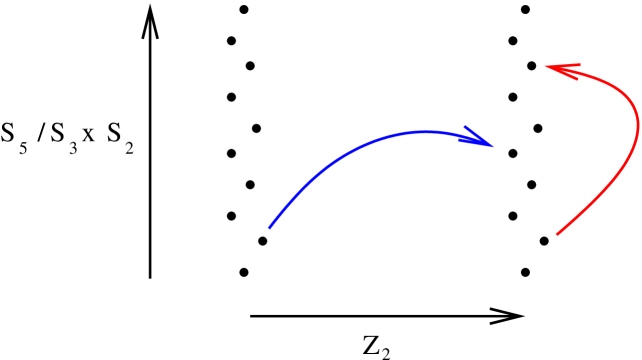
Figure 1: The vacuum manifold of the model consists of $10+10$ points. Domain walls correspond to solutions interpolating between any two vacua. There are two kinds of domain walls, one interpolating between the two sets of 10 vacua related by $Z_{2}$ transformations, and the other interpolating between vacua within a set of 10 vacua. If we fix the vacuum at $x=-\infty$ there are 10 ways of choosing the vacuum at $x=+\infty$ that differs by a $Z_{2}$ transformation, leading to 10 different $Z_{2}$ walls. Of these 10 $Z_{2}$ walls, 3 are of lowest energy, 6 are of intermediate energy, and 1 has the highest energy PogVac01 .

In Ref. PogVac03 it was shown that walls and antiwalls of different type repel in this model. This led to the possibility of a stable lattice of alternating domain walls and antiwalls provided that all the neighboring walls and antiwalls are of different type. If a neighboring wall and antiwall are of the same type, they will attract, then annihilate. The lattice can be schematically depicted as in Fig. 2 or by the sequence of vacuum configurations:

$$... \rightarrow +(2,2,2,-3,-3)\rightarrow-(2,-3,-3,2,2)$$ (7)

$$\rightarrow +(-3,2,2,-3,2)\rightarrow-(2,-3,2,2,-3)$$

$$\rightarrow +(2,2,-3,-3,2)\rightarrow-(-3,-3,2,2,2)$$

$$\rightarrow +(2,2,2,-3,-3)\rightarrow...$$

This sequence gives the minimal lattice of 6 kinks.

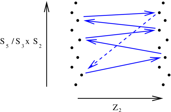
Figure 2: Depiction of the sequence of vacuum configurations in the domain wall lattice.

In our one dimensional simulations AntPogVac04 we found that a domain wall lattice is inevitably formed after a phase transition provided the compact dimension is not too small. In our preliminary work in two equal compact spatial dimensions ($L_{y}=L_{x}$) we had found that a domain wall network with junctions is formed after the phase transition and this network coarsens, eventually ending in the vacuum. In other words, a domain wall lattice was not seen to form. The present paper deals with the case of two unequal compact spatial dimensions ($L_{y}\neq L_{x}$). We expect that when one of the dimensions is very small, the system will behave like the one dimensional case, and a lattice will almost certainly be formed. When the sizes of the two dimensions are comparable, based on the preliminary results, we would not expect a lattice to form. This will turn out to be incorrect and our more extensive analysis will show that even in the $L_{y}=L_{x}$ case there is a small chance of lattice formation. We will be interested in determining the domain wall lattice characteristics as a function of the relative sizes of the dimensions of the compact space.

III Numerical technique

In our simulations we try to mimic some features of a typical non-equilibrium second order phase transition. In order to do that we use a Langevin-type equation based on the fundamental Lagrangian of the theory Eq. (2):

$$\left(\partial_{t}^{2}-\nabla^{2}\right)f_{i}+\partial_{i}V+D\,\partial_{t}f_{i}=\Gamma_{i},$$ (8)

The Langevin equation describes the evolution of the system coupled to a heat bath with temperature $T$. The effect of the bath is modeled by including in the equations of motion a dissipation term with dissipation constant $D$, and a stochastic force $\Gamma_{i}(x,t)$. The stochastic force is a Gaussian distributed field obeying:

$$\langle\Gamma_{i}(x,t)\rangle=0,$$

$$\langle\Gamma_{i}(x,t)\Gamma_{j}(x^{\prime},t^{\prime})\rangle=2DT\,\delta_{ij}\delta(x-x^{\prime})\delta(t-t^{\prime})$$ (9)

The amplitude of the noise in Eq. (9) is chosen so as to guarantee that independently of the initial field configuration and of the particular value of the dissipation, the system will always equilibrate toward a thermal distribution with temperature $T$.

In a typical simulation, we start with an arbitrary initial condition and evolve Eq. (8) for a period of time long enough for the system to equilibrate. We then mimic an instantaneous phase transition to $T=0$ temperature, by setting the noise term in Eq. (8) to zero. In the subsequent period of evolution, the dissipation forces the fields to its possible vacua values, and a complex network of domain walls forms, separating different vacuum regions. This network is then allowed to evolve until a final stable state is reached. A detailed discussion on how the evolution proceeds can be found in AntPogVac04 .

The equations of motion were discretized using a standard leapfrog method and periodic boundary conditions were used. The model parameters were set to $m=1/(2\sqrt{6})$, $\lambda=1/2$ and $h=-3/40$. For this particular choice of parameters there is a known explicit analytical solution for the relevant domain profile PogVac00 ; Vac01 . The lattice spacing was $\delta x=1.$ and the time-step set to $\delta t=.5$. For the parameters above, the wall core is resolved by more that 10 lattice points which should be accurate enough for the desired purposes. The value of the dissipation coefficient $D$ does not influence the results during the stochastic stage of the simulation and we set it to $D=.5$ to ensure rapid thermalization. We keep the same dissipation value during the evolution regime at $T=0$, the reasons behind this choice and its effects on the final results are discussed in detail in the next Section.

In order to identify the walls during and at the end of the simulation, we convert the $f_{i}(x)$’s back into their original $SU(5)\times Z_{2}$ matrix form, $\Phi(x)$, via Eq. (4). It is easy to see that for the lowest energy kinks in the model, the sign of ${\rm Tr}[\Phi^{3}]$ vanishes at the defect core AntPogVac04 . For these kinks, one (and only one) of the fields $\Phi_{jj}$ crosses zero at the core as well. In the simulation we measure, at each time-step, the value of ${\rm Tr}[\Phi^{3}]$ and look for pairs of neighboring lattice points for which this quantity changes sign. In these cases we determine which of the field components goes through zero. This way we are able both to find the domain walls and to identify them according to their five possible charges, as described in Section II.

All the simulations were run in two-dimensional domains with periodic boundary conditions. For each set of runs, the size of the simulation box in the $x$-direction was fixed to a constant $L_{x}$, whereas its $y$ dimension, $L_{y}$ was allowed to vary. For each choice of $L_{x}$ and $L_{y}$, we executed several independent runs with different random seeds and averaged the relevant physical quantities over those to obtain the final results.

IV Results

In Fig. 3 we have an example of how the evolution of a typical network of walls proceeds in a toroidal domain. In this case, the larger dimension was set to $L_{x}=500$ and the smaller to $L_{y}=150$. For early times after the temperature is quenched to zero (top plot, $t=500$), we can observe a dense population of walls forming a complex network. While it is not obvious from the topology of the vacuum manifold that domain wall junctions (“nodes”) exist in the model Davetal02 , the simulation clearly shows their presence. These nodes may be viewed as being due to the existence of domain wall lattices in one dimension. To see this, imagine a circle in two spatial dimensions. It is possible to have a lattice of walls on this circle. Now if we shrink the circle to a point, the walls forming the lattice have to converge to a point. In other words, the walls on one of the circles are like spokes on a wheel and have to necessarily have a point of convergence in two dimensions. While an infinite number of lattice configurations can be constructed, the minimal number of walls in a stable lattice is six. In the simulation also we see that a majority of intersecting nodes consist of six incoming walls. As the evolution proceeds, several mechanisms play a role in decreasing the overall wall density. Walls and anti-walls of the same type annihilate each other and closed loops can be formed later decaying into radiation. The intersecting nodes are also dynamical and can disentangle when nodes and anti-nodes collide. A snapshot of the wall network for intermediate times can be seen in the middle plot in Fig. 3. Finally, for long times, all the loops collapse and all nodes annihilate, leaving behind a set of straight parallel walls wrapped around the shortest dimension of the simulation torus. Depending on their charge, some of these walls may still annihilate each-other, and the final state of the evolution is either the vacuum or a lattice of equidistant repelling walls. In the bottom plot of Fig. 3 we can see that for $t=5000$ the system has relaxed into a stack of parallel walls. Since we know how to identify the wall charge from the simulation data, once this stage of the evolution is reached it is straightforward to predict which walls will annihilate and how many (if any) will remain in the final lattice. In this particular case there is only one wall anti-wall pair that annihilates, resulting in a lattice of 10 walls.

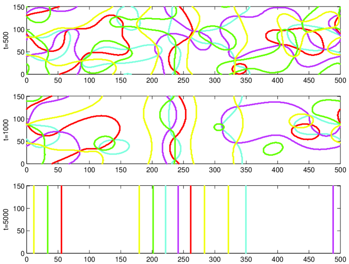
Figure 3: The domain wall network for three typical stages in an evolution in a toroidal domain, with dimensions $L_{x}=500$ and $L_{y}=150$. The different shades correspond to the $5$ possible charges the domain walls can have in the theory. Note that in the bottom figure there is a pair of neighboring wall and anti-wall of the same type (the walls just before and after the $300$ mark). These will later on annihilate each other leading to a final stable lattice consisting of $10$ walls.

Though the pattern of the evolution remains the same independently of the relative dimensions of the two-dimensional torus, its final outcome depends markedly on the values of $L_{x}$ and $L_{y}$.

The most striking trend in the data is that the final state of the evolution is very likely to be a stable wall lattice when $L_{y}\ll L_{x}$, whereas the vacuum state is the predominant outcome when the two dimensions are comparable. This dependence is illustrated more explicitly in Fig. 4, where we show the probability of having a lattice forming as a function of the ratio of the two dimensions of the simulation domain. For each choice of $L_{x}$ and $L_{y}$, the formation probability is defined as the number of independent runs that led to the formation of a lattice, divided by the total number of runs. For the three fixed choices of the largest dimension, $L_{x}=100$, $300$, and $500$, the results were obtained by averaging over $64$, $40$ and $40$ runs for each value of the smallest dimension $L_{y}$. In all three cases, $L_{y}$ was varied from $0$ to a larger value, close to $L_{x}$ in the two cases of small $L_{x}$ but only to about $250$ for $L_{x}=500$ (the reason being that for the larger case it takes a very long time for the system to reach its final state, and simulations for higher $L_{y}$ become numerically demanding). The errors calculated from the standard deviation of the data are of the same magnitude as the results. We chose not to show them in the plot (and likewise in the following figures) so not to obscure the results.

For $L_{y}=0$, the probability of forming a lattice is quite high, being in fact equal to unity in the case of $L_{x}=500$. This is to be expected since this case corresponds to having the evolution taking place in a one-dimensional domain. As was shown in PogVac03 , in 1D, as the size of the physical domain goes to infinity, the probability of forming a lattice tends to one. On the other hand, for the symmetric $2D$ system where $L_{x}=L_{y}$, the lattice formation probability is quite small. In the case of the $L_{x}=L_{y}=100$ simulations, out of $64$ independent runs only $3$ had a stable lattice of walls as their final state. A similar result was found for the $L_{x}=L_{y}=200$ case, where $3$ lattices were formed in a total of $32$ simulations. We also observed that in the few cases where a lattice is formed in a $L_{x}=L_{y}$ box, the lattice shows no preferred direction of alignment. In the low and medium range of $L_{y}/L_{x}$ on the contrary, the walls in the final lattice are always parallel to the $y$ direction, as expected (see Fig. 3). For $L_{x}=200$ the first lattices in the $x$ direction appear only for $L_{y}=150$ whereas for $L_{x}=100$ these are observed for values of the $y$ dimension larger than $L_{y}=70$.

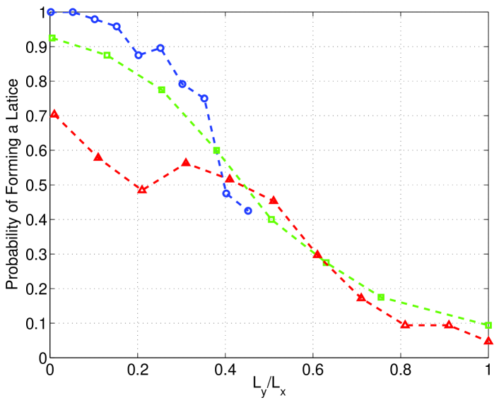
Figure 4: Probability of forming a lattice of domain walls as a function of the ratio of the two torus dimensions. $L_{x}$ is fixed for each curve, taking the values $500$ (circles), $200$ (squares) and $100$ (triangles). Standard deviation error bars (not shown for clarity) are of the same order of magnitude as the result.

It is interesting to note that the formation probability for large values of the ratio $R\equiv L_{y}/L_{x}$ seems to be independent of the choice of $L_{x}$. A similar effect can be seen in the averaged number of walls in the final state, as plotted in Fig. 5. The curves for the three choices of $L_{x}$ converge for a value of roughly $L_{y}/L_{x}=0.4$ and coincide above that. Other quantities seem to follow the same pattern in this regime. The size ratio above which walls parallel to the larger dimension are found in the final state, is given by $R=150/200=0.75$ in the case $L_{x}=200$. For the smaller box $L_{x}=100$, the result is similar with walls in the $x$ direction appearing above $R=70/100=0.70$

The outcome of the evolution clearly seems to vary within two well defined regimes. For $R>0.4$ the properties of the final state depend only on the ratio of the dimensions of the compact space, whereas for lower values of $R$ the results depend also on $L_{x}$. In the small $R$ regime, for example, the final number of walls varies considerably. That this is to be expected can be easily seen by considering the $L_{y}=0$ limit, corresponding to the one-dimensional case. In this situation we would expect the final number of walls to be proportional to the length of the 1D domain. In other words, the final wall density $\rho$ – defined as the total length in walls divided by the area of the lattice – should depend little on $L_{x}$, which is indeed observed:

$$\rho_{100}=0.047,\,\,\,\,\,\,\,\rho_{200}=0.046,\,\,\,\,\,\,\,\rho_{500}=0.042$$ (10)

As shown in Fig. 6 the curves for the number density are quite close to each other for small values of $L_{y}/L_{x}$, diverging for higher ratios of the two dimensions.

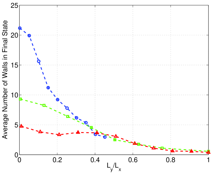
Figure 5: Average number of walls in the final stable configuration. The spatial dimensions of the torus are the same as in Fig. 4. Standard deviation error bars (not shown for clarity) are of the same order of magnitude as the result.

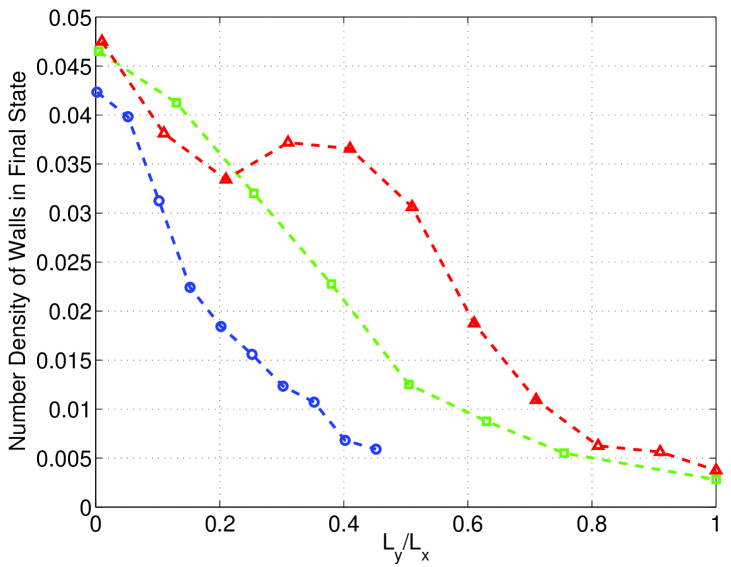
Figure 6: Total wall length per unit area in the final stable configuration. The spatial dimensions of the torus are the same as in Fig. 4. Standard deviation error bars (not shown for clarity) are of the same order of magnitude as the result.

Finally we note that, as mentioned in Section III, a non-zero dissipation term is kept throughout the whole evolution. We expect that the presence of dissipation, though changing the type of scaling of the dynamics of the network, should not influence qualitatively the outcome of the evolution. The reason for this is that the probability of forming a lattice should depend mostly on the number of uncorrelated domains in the initial state of the evolution. As a check, we ran a few simulations with dissipation set to zero during the evolution stage. The final results turned out to be different from the above, but only for small values of $L_{x}$ and $R$. The reason behind this is that after the quench there is still a lot of energy stored in the field which can be re-distributed among its different degrees of freedom. One consequence of this process is that it can effectively destroy the initial pattern of vacuum domains. For example, in the $L_{x}=500$, $L_{y}=0$ case, the formation probability is still unity but the average wall number in the final state is less than shown in Fig. 4. This observation can be interpreted as a consequence of the effective domain size being changed soon after the quench, when the dissipation is turned off. This would also explain why the effects vanish for larger boxes. The conclusion is that keeping the dissipation on during the evolution allows us to use smaller simulation boxes to probe the large scale limit of theory.

V Summary

We have numerically studied phase transitions in a model with $S_{5}\times Z_{2}$ symmetry breaking down to $S_{3}\times S_{2}$ in two compact spatial dimensions. As expected, the outcome depends on the ratio of the sizes of the two dimensions: $R\equiv L_{y}/L_{x}$. As $R\rightarrow 0$, the system behaves as in one spatial dimension and a domain wall lattice forms. As $R\rightarrow 1$, the system behaves as in two spatial dimensions and a domain wall lattice rarely forms. What is surprising though is that the critical value of $R$ below which a lattice forms with large probability is of order unity: $R_{c}\sim 0.4$.

In earlier work AntPogVac04 we have studied the evolution of the network in time and found that the total length of the network falls off as $t^{-0.7}$ in the $L_{y}=L_{x}$ ($R=1$) case. Here we have focused on the late time state of the system with various values of $R$ and have determined the domain wall density $\rho$ at late times as a function of $R$. At the moment we do not know if there are naturally occurring systems in which a domain wall lattice exists. The domain wall lattice may also be relevant for cosmology, possibly in the context of brane cosmology.

- (1) T. Garagounis and M. Hindmarsh, Phys. Rev. D68, 103506 (2003).
- (2) B.S. Ryden, W.H. Press and D.N. Spergel, Ap. J. 357, 293 (1990).
- (3) H. Kubotani, H. Ishihara and Y. Nambu, in Primordial Nucleosynthesis and Evolution of Early Universe. Edited by K. Sato and J. Audouze. Dordrecht, Netherlands, Kluwer Academic, 1991
- (4) H. Kubotani, Prog. Theor. Phys. 87, 387 (1992).
- (5) L. Pogosian and T. Vachaspati, Phys. Rev. D62, 123506 (2000).
- (6) T. Vachaspati, Phys. Rev. D63, 105010 (2001).
- (7) L. Pogosian and T. Vachaspati, Phys. Rev. D64, 105023 (2001).
- (8) L. Pogosian, Phys. Rev. D65, 065023 (2002).
- (9) A. Davidson, B. F. Toner, R. R. Volkas and K. C. Wali, Phys. Rev. D65, 125013 (2002).
- (10) D. Tong, Phys. Rev. D66, 025013 (2002).
- (11) L. Pogosian and T. Vachaspati, Phys. Rev. D67, 065012 (2003).
- (12) T. Vachaspati, hep-th/0303137.
- (13) N. D. Antunes, L. Pogosian and T. Vachaspati, Phys. Rev. D69, 043513 (2004).