V–A sum rules with D=10 operators

Abstract

The difference of vector and axial-vector charged current correlators is analyzed by means of QCD sum rules. The contribution of 10-dimensional 4-quark condensates is calculated and its value is estimated within the framework of factorization hypothesis. It is compared to the result, obtained from operator fit of Borel sum rules in the complex $q^{2}$-plane, calculated from experimental data on hadronic $\tau$-decays. This fit gives accurate values of the light quark condensate and quark-gluon mixed condensate. The size of the high-order operators and the convergence of operator series are discussed.

1 Introduction

The QCD sum rules SVZ have been widely used for the determination of fundamental theoretical parameters, such as the coupling constant $\alpha_{s}$, quark masses and various nonperturbative condensates. Their accuracy depends on experimental errors and theoretical uncertainties. In many cases both experimental and theoretical errors are comparable by the order of magnitude, and any improvement is of interest.

In this paper we will consider the 2-point correlators of charged vector and axial-vector currents, constructed from light $u$,$d$-quarks:

$$\Pi^{U}_{\mu\nu}(q)\,=\,i\int dx\,e^{iqx}\left<TU_{\mu}^{\dagger}(x)U_{\nu}(0)\right>$$

$$\,=\,(q_{\mu}q_{\nu}-g_{\mu\nu}q^{2})\,\Pi^{(1)}_{U}(q^{2})\,+\,q_{\mu}q_{\nu}\,\Pi^{(0)}_{U}(q^{2})$$ (1)

where

$$U=V,A:\qquad V_{\mu}={\bar{u}}\gamma_{\mu}d\;,\;A_{\mu}={\bar{u}}\gamma_{\mu}\gamma^{5}d\;.$$

The polarization functions $\Pi^{(i)}(s)$ have a cut along the real axes in the complex $s=q^{2}$ plane. Their imaginary parts (spectral functions)

$$v_{1}/a_{1}(s) = 2\pi\,{\rm Im}\,\Pi^{(1)}_{V/A}(s+i0)\;,$$

$$a_{0}(s) = 2\pi\,{\rm Im}\,\Pi^{(0)}_{A}(s+i0)$$ (2)

have been measured for $0<s<m_{\tau}^{2}$ by ALEPH ALEPH and OPAL OPAL collaborations from hadronic decays of $\tau$-lepton.

Of particular interest is the difference $\Pi_{V}^{(1)}-\Pi_{A}^{(1)}$, since it does not contain any perturbative contribution in the massless quark limit. The experimental data on the difference $v_{1}(s)-a_{1}(s)$ are shown in Fig. 1. As demonstrated in IZ , the dispersion relation can be written in the following form:

$$\Pi_{V}^{(1)}(s)-\Pi_{A}^{(1)}(s) = {1\over 2\pi^{2}}\int_{0}^{\infty}{v_{1}(t)-a_{1}(t)\over t-s}\,dt\,+\,{f_{\pi}^{2}\over s}$$ (3)

$$= \sum_{D\geq 4}{O_{D}^{V-A}\over(-s)^{D/2}}$$

where the sum goes over even dimensions $D$ of the operators (condensates) $O_{D}$. The term $f_{\pi}^{2}\over s$, $f_{\pi}=130.7\,{\rm MeV}$ is the pion decay constant, is the kinematical pole of the axial polarization function $\Pi^{A}_{\mu\nu}$, see IZ for details. In (3) and below the notation $O_{D}^{V-A}$ stands for the condensates with all $\alpha_{s}$ corrections, including slowly varying logarithmic terms $\sim\ln^{n}(-s)$. The list of the condensate contribution to the vector and axial correlators separately can be found in BNP .

The sum rules for the difference (3) have been studied in IZ , DGHS –RL where the lowest order condensates $O_{D}^{V-A}$ were found. Although the published values of $O_{6}^{V-A}$ are close to each other (within the errors), this is not the case for the operator $O_{8}^{V-A}$. In IZ , DGHS positive values of the $D=8$ condensate were found, but the authors of recent publications CGM , RL have obtained negative condensate $O_{8}^{V-A}$. The source of this discrepancy could be very large condensates of dimension $D=10$ and higher, accounted in CGM , RL : a typical ratio of the condensates in these papers is $|O_{2n+2}/O_{2n}|\sim 5-10\,{\rm GeV}^{2}$. If this statement is correct, the OPE analysis of IZ would be invalid, because the contribution of unknown high-order terms was estimated from the assumption $|O_{10}/O_{6}|\lesssim 1-2\,{\rm GeV}^{4}$. For this reason it would be interesting to find the operator $O_{10}^{V-A}$ independently and compare it with the sum rule results.

In this paper we repeat the analysis of IZ with the $D=10$ operator included. In Section 2 all necessary $V-A$ operators, obtained from the Operator Product Expansion in QCD, are listed and their values are estimated within the framework of the factorization hypothesis. In Section 3 the operator values are obtained from the fit to Borel sum rules. In the last Section the validity of our assumptions is discussed and the results are compared with the ones obtained in other publications. The complete form of the $D=10$ operator and technical details of its derivation are dropped to Appendices A,B.

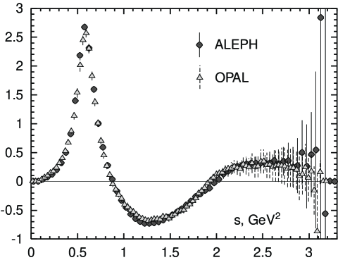
Figure 1: Spectral function $v_{1}(s)-a_{1}(s)$ obtained from ALEPH ALEPH and OPAL OPAL data

2 V–A operator expansion

The first term in the operator series (3) is the $D=4$ operator:

$$O_{4}^{V-A} = 2(m_{u}+m_{d})\langle{\bar{q}}q\rangle$$ (4)

$$\times \left[\,1\,+\,{4\over 3}\,{\alpha_{s}(Q^{2})\over\pi}+\,{59\over 6}\left({\alpha_{s}(Q^{2})\over\pi}\right)^{2}\,\right]$$

where $Q^{2}=-q^{2}$, we assume $\langle{\bar{u}}u\rangle=\langle{\bar{d}}d\rangle\equiv\langle{\bar{q}}q\rangle$. The $\alpha_{s}$ corrections have been computed in Gen and CGS . In fact, the contribution of the $D=4$ operator to the sum rules considered here, is small. So we can safely neglect the $\alpha_{s}$-corrections in (4) and put $O_{4}^{V-A}=-f_{\pi}^{2}m_{\pi}^{2}=-3.3\times 10^{-4}\,{\rm GeV}^{4}$, as follows from Gell-Mann-Oakes-Renner low energy theorem GMOR .

The $D=6$ operator in factorized form is equal to:

$$O_{6}^{V-A}=-8\pi C_{N}\alpha_{s}\langle{\bar{q}}q\rangle^{2}\left[1+{\alpha_{s}(\mu^{2})\over\pi}\left(c_{6}-{1\over 4}\ln{Q^{2}\over\mu^{2}}\right)\right]$$ (5)

where $C_{N}=1-N_{c}^{-2}=8/9$ is the color factor, which appears in the factorization of the 4-quark operators at the leading $\alpha_{s}$-order. The NLO terms were computed in LSC and the constant $c_{6}$ was found equal to $247/48$. In AC another treatment of $\gamma^{5}$ matrix in dimensional regularization was employed, leading to $c_{6}=89/48$. For the later choice at $\mu=1\,{\rm GeV}$ and $\alpha_{s}(\mu^{2})=0.5$ one finds the factor in square brackets in (5) equal to 1.3 (the logarithmic term can be neglected due to small numerical coefficient).

The contribution of the $D=8$ 4-quark condensates to the vector current correlator was originally obtained in DS in factorized form and in GP in complete (nonfactorized) form. In IZ these results were verified and an ambiguity of the factorization at the $N_{c}^{-2}$ order was pointed out. Here we will follow the factorization procedure, described in Appendix B. The result is:

$$O_{8}^{V-A}\,=\,8\pi C_{N}\alpha_{s}m_{0}^{2}\langle{\bar{q}}q\rangle^{2}\;,$$ (6)

where the mass $m_{0}$ is defined from the 5-dimensional quark-gluon mixed condensate:

$$i\langle{\bar{q}}\hat{G}q\rangle\,=2\langle{\bar{q}}D^{2}q\rangle\,=\,-\,m_{0}^{2}\langle{\bar{q}}q\rangle$$ (7)

where $\hat{G}=\gamma_{\alpha}\gamma_{\beta}G_{\alpha\beta}$, $G_{\alpha\beta}=i[D_{\alpha},D_{\beta}]$ is the gluon field strength, see Appendix A for more definitions. The parameter $m_{0}^{2}$ has a meaning of typical momentum of virtual quarks in vacuum. It was found from baryonic sum rules $m_{0}^{2}=0.8\pm 0.2\,{\rm GeV}^{2}$ BI ; DJN , and $B-B^{*}$ splitting Nar . The values close to $1\,{\rm GeV}^{2}$ were also obtained from the latest lattice calculation ChH and in QCD string model DiGS .

There are many different condensates of dimension $D=10$. They can be grouped into four parts:

$$O_{10}^{V-A}\,=\,O^{(0)}_{10}\,+\,O^{(2)}_{10}\,+\,O^{(4)}_{10}\,+\,O^{(6)}_{10}$$ (8)

where upper index $(i)$ denotes the number of quarks in vacuum. This separation is shown diagrammatically in Fig. 2. The purely gluonic operators $O^{(0)}$ and the 2-quark ones $O^{(2)}$ cancel in the $V-A$ correlator in the limit of massless $u,d$-quarks. The operators with 6 quarks in vacuum have the structure $\langle({\bar{q}}q)^{2}({\bar{q}}Dq)\rangle$. After factorization they become $\sim m\langle{\bar{q}}q\rangle^{3}$, which is again negligible for light quarks. The only essential contribution to the $V-A$ sum rules comes from the 4-quark operators $O_{10}^{(4)}$.

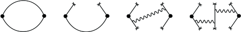
Figure 2: Condensate expansion (8) by the number of quarks in vacuum. Circles stand for the currents $V/A$, crosses are quarks in vacuum; gluons in vacuum are not shown.

In this paper we have computed the contribution of the 4-quark condensates to the vector and axial current correlator. Details of calculation and complete form of the operator $O_{10}^{(4)}$ are given in Appendix A. The factorization scheme necessary to reduce large number of independent structures, is described in Appendix B. The result is:

$$O_{10}^{V-A} = \pi\alpha_{s}C_{N}\left[\,{50\over 9}\,\langle{\bar{q}}\hat{G}q\rangle^{2}\right.$$ (9)

$$\left.-\,16\left(\,3\,X_{1}\,-\,X_{2}\,+\,X_{3}\,+\,{7\over 6}\,X_{4}\,\right)\langle{\bar{q}}q\rangle\,\right]$$

where $X_{i}$ are 4 independent $D=7$ quark-gluon condensates:

$$X_{1}=\langle{\bar{q}}G_{\alpha\beta}G_{\alpha\beta}q\rangle,\qquad\;\;X_{2}=i\langle{\bar{q}}\gamma^{5}G_{\alpha\beta}{\tilde{G}}_{\alpha\beta}q\rangle,\;$$

$$X_{3}=\langle{\bar{q}}\gamma_{\alpha\beta}G_{\alpha\gamma}G_{\beta\gamma}q\rangle,\quad X_{4}=i\langle{\bar{q}}\gamma_{\alpha\beta}(D_{\alpha}J_{\beta})q\rangle.$$ (10)

where $\tilde{G}_{\alpha\beta}$ is the dual gluon-field strength, $\gamma_{\alpha\beta}={1\over 2}(\gamma_{\alpha}\gamma_{\beta}-\gamma_{\beta}\gamma_{\alpha})$ and $J_{\alpha}=D_{\beta}G_{\alpha\beta}$. Their numerical values are not known. The condensate $X_{4}$ can be brought to the 4-quark form $X_{4}\sim\langle({\bar{q}}q)({\bar{q}}Dq)\rangle\sim m\langle{\bar{q}}q\rangle^{2}$, which is negligible. In order to estimate other condensates, we assume further factorization according to $\langle{\bar{q}}\Gamma q\rangle=\langle{\bar{q}}q\rangle\,\langle{\rm tr}\,\Gamma\rangle/(4N_{c})$, the trace is taken both over color and spinor indices. Then:

$$X_{1}\,=\,{2\pi\over 3}\,\alpha_{s}\left<G_{\alpha\beta}^{a}G_{\alpha\beta}^{a}\right>\langle{\bar{q}}q\rangle\;,\qquad X_{2}\,=\,X_{3}\,=\,X_{4}\,=\,0\;.$$ (11)

Under these assumptions the operator (9) takes the form:

$$O_{10}^{V-A}\,=\,-\,\pi\alpha_{s}C_{N}\langle{\bar{q}}q\rangle^{2}\left[\,{50\over 9}\,m_{0}^{4}\,+\,32\pi\alpha_{s}\left<G^{2}\right>\,\right]$$ (12)

It is rather difficult to find accurate value of the gluon condensate from any sum rule. Detailed analysis of charmonium sum rules performed in IZ2 has lead to the restriction $\langle{\alpha_{s}\over\pi}G^{2}\rangle=0.009\pm 0.007\,{\rm GeV}^{4}$, in agreement with many previous estimations. Taking this central value and $m_{0}^{2}=1\,{\rm GeV}^{2}$, one obtains $O_{10}^{V-A}/O_{6}^{V-A}=0.8\,{\rm GeV}^{4}$. For $O_{6}^{V-A}=-(6.8\pm 2.1)\times 10^{-3}\,{\rm GeV}^{6}$ IZ we find the following estimation of the $D=10$ $V-A$ condensate:

$$O_{10}^{V-A}\,=\,-5\times 10^{-3}\,{\rm GeV}^{10}$$ (13)

In the next section we will compare this estimation with results of the fit, obtained from the sum rules.

3 V–A sum rules

Many different sum rules have been investigated in order to determine numerical values of the condensates. Most of authors employ polynomial sum rules: the correlator $\Pi^{(1)}_{V}(s)-\Pi^{(1)}_{A}(s)$ is multiplied on some polynomial of $s$ and then integrated over the circle $|s|=s_{0}$ in the complex $s$-plane. Their advantages are: 1) one does not need to know the spectral function $v_{1}(s)-a_{1}(s)$ for $s>s_{0}$, which allows to reduce high error from the region $s\approx m_{\tau}^{2}$ by choosing $s_{0}$ reasonably below $m_{\tau}^{2}$ and 2) all operators of dimension higher then the polynomial dimension, do not enter these sum rules due to Cauchy theorem. But the disadvantages are also obvious. If the operator expansion (3) is divergent (asymptotic), the Cauchy theorem is not applicable to this series. Moreover, possible logarithmical terms $\sim\ln^{k}\!Q^{2}/Q^{2n}$ appear at the NLO in $\alpha_{s}$ expansion. These terms contribute to any polynomial sum rules. It makes uncontrollable the contribution of the high order operators to the polynomial sum rules at $s_{0}\lesssim 2\,{\rm GeV}^{2}$, especially for large ones as obtained in CGM ; RL .

For these reasons we prefer Borel sum rules, where the high order operators are suppressed as $O_{2n}/n!$. In order to separate out the contributions of different operators from each other, one may consider the Borel transformation in the complex plane of the Borel mass $M^{2}\to M^{2}e^{i(\pi-\phi)}$ (which is equivalent to the Borel operator applied to the dispersion relation (3) written along the ray $s\to se^{i\phi}$ in the complex $s$-plane IZ ). The real and imaginary parts of the Borel transformation are:

$$\int_{0}^{s_{m}}\!\exp{\left({s\over M^{2}}\cos{\phi}\right)}\cos{\left({s\over M^{2}}\sin{\phi}\right)}\,(v_{1}-a_{1})(s)\,{ds\over 2\pi^{2}}$$

$$\qquad=\,f_{\pi}^{2}+\sum_{k=1}^{\infty}(-)^{k}{\cos{(k\phi)}\,O_{2k+2}^{V-A}\over k!\,M^{2k}}$$ (14)

$$\int_{0}^{s_{m}}\!\exp{\left({s\over M^{2}}\cos{\phi}\right)}\sin{\left({s\over M^{2}}\sin{\phi}\right)}\,(v_{1}-a_{1})(s)\,{ds\over 2\pi^{2}M^{2}}$$

$$\qquad=\,\sum_{k=1}^{\infty}(-)^{k}{\sin{(k\phi)}\,O_{2k+2}^{V-A}\over k!\,M^{2k+2}}$$ (15)

We made the imaginary part (15) dimensionless, while the real part (14) has dimension ${\rm GeV}^{2}$ in order to separate out the leading constant term $f_{\pi}^{2}$. The logarithmical terms are neglected in the rhs of (14,15), otherwise the terms $\sim\ln{M^{2}}$ appear. The only known logarithmical term is in the $\alpha_{s}$-correction to the $D=6$ operator (5). It can be easily taken into account (see CGM for explicit formulae), but its relative contribution is negligible due to small numerical factor, so we shall ignore it.

The derivation of (14,15) from the dispersion relation (3) implies infinite upper integration limit $s_{m}=\infty$. Experimental data on the axial function $a_{1}(s)$ are available only for $s<m_{\tau}^{2}=3.16\,{\rm GeV}^{2}$. However the data at $s>3\,{\rm GeV}^{2}$ are rather unstable and have large error because of low statistics, see Fig 1. For this reason we put $s_{m}=3.0\,{\rm GeV}^{2}$ in (14,15). Removal of the data above this point does not change the Borel transform significantly (if $M^{2}$ is not sufficiently large), but may reduce the errors. In fact, the sum rules considered here do not rely on the high-energy data: say, if the upper integration limit $s_{m}$ is reduced to $2.5\,{\rm GeV}^{2}$, the condesates change at most within $10\%$ limit. If the data above $3\,{\rm GeV}^{2}$ are removed, both ALEPH and OPAL data give almost equal central values and similar errors of the Borel transforms (14,15). For this reason we will psesent below the analisys of ALEPH data only, since they have smaller errors. The condensates, obtained from OPAL data are almost the same.

The argument of the exponent must be negative $\cos{\phi}<0$ in order to suppress contribution of the high-energy states from unknown region $s>m_{\tau}^{2}$, which means $\pi/2<\phi<\pi$. Of special interest are the closest to $\pi$ (minimal error) angles at which the contribution of some operator $O_{2k+2}$ vanishes. Such angles are $\phi=\pi(2k-1)/(2k)$, $k=2,3,\ldots$ for real part (14) and $\phi=\pi(k-1)/k$, $k=3,4,\ldots$ for imaginary one (15). The sum rules (14,15) at some of these angles were considered in IZ with the operators $O_{6}$ and $O_{8}$ as free parameters to fit. It was shown, that for $O_{6}^{V-A}=-(6.8\pm 2.1)\times 10^{-3}\,{\rm GeV}^{6}$ and $O_{8}^{V-A}=(7\pm 4)\times 10^{-3}\,{\rm GeV}^{6}$ they are well satisfied for $M^{2}>0.6\,{\rm GeV}^{2}$.

$$\begin{array}[]{c|c|ccc|c}\hline\cr\phi&\;M^{2},\,{\rm GeV}^{2}&O_{6}^{V-A}&O_{8}^{V-A}&O_{10}^{V-A}&\chi_{0}^{2}\\ \hline\cr\hline\cr 2\pi/3&\begin{array}[]{c}0.4-1.0\\ 0.5-1.0\end{array}&\;\begin{array}[]{c}-7.0\pm 1.4\\ -7.0\pm 2.5\end{array}&&\;\begin{array}[]{c}-3.8\pm 3.3\\ -3.9\pm 10.3\end{array}&\;\begin{array}[]{c}0.14\\ 0.14\end{array}\\ \hline\cr 3\pi/4&\begin{array}[]{c}0.4-1.0\\ 0.5-1.0\end{array}&\;\begin{array}[]{c}-7.3\pm 1.1\\ -7.9\pm 2.3\end{array}&\;\begin{array}[]{c}8.0\pm 2.1\\ 9.5\pm 2.5\end{array}&&\;\begin{array}[]{c}0.17\\ 0.12\end{array}\\ \hline\cr 4\pi/5&\begin{array}[]{c}0.3-1.0\\ 0.4-1.0\end{array}&\;\begin{array}[]{c}-8.1\pm 1.8\\ -9.3\pm 5.1\end{array}&\;\begin{array}[]{c}10.3\pm 4.1\\ 13.8\pm 15.1\end{array}&\;\begin{array}[]{c}-7.6\pm 5.0\\ -13.2\pm 23.8\end{array}&\;\begin{array}[]{c}0.11\\ 0.06\end{array}\\ \hline\cr\hline\cr{\rm all}&&\;\begin{array}[]{c}-7.2\pm 1.2\\ -7.5\pm 2.3\end{array}&\;\begin{array}[]{c}7.8\pm 2.5\\ 8.6\pm 6.0\end{array}&\;\begin{array}[]{c}-4.4\pm 2.8\\ -5.2\pm 8.4\end{array}&\;\begin{array}[]{c}0.40\\ 0.20\end{array}\\ \hline\cr\end{array}$$

Table 1: Operator fit obtained from eq (15) for different angles $\phi$; operators are in $10^{-3}\,{\rm GeV}^{D}$. Last two lines contain combined fits for all these angles for upper/lower choice of $M^{2}$ range.

It is more difficult to find high-order condensates (say $O_{10}^{V-A}$) from the sum rules, since several unknown parameters enter the same equation and the high-order condensate strongly depends on exact values of the low-order ones. Here one needs to consider the Borel transformation at several values of $M^{2}$, where the relative contributions of various condensates are different. In other words, we may fit the shape of theoretical curve with experimental one within some reasonable region $M_{1}^{2}<M^{2}<M_{2}^{2}$. For this purpose it is natural to define the least square deviation, normalized to experimental error:

$$\chi^{2}\,=\,{1\over M_{2}^{2}-M_{1}^{2}}\int_{M_{1}^{2}}^{M_{2}^{2}}dM^{2}\,\left({B^{theor}-B^{exp}\over\Delta B^{exp}}\right)^{2}$$ (16)

where $B^{theor}/B^{exp}$ is the right/left hand side of the Borel sum rules (14,15). One may calculate $\chi^{2}$ with theoretical condensates $O_{i}$ as free parameters. It is quadratic function of them:

$$\chi^{2}\,=\,\chi^{2}_{0}\,+\,\sum_{i,j}C_{ij}\left(O_{i}-\overline{O}_{i}\right)\left(O_{j}-\overline{O}_{j}\right)$$ (17)

Obviously $\overline{O}_{i}$ are the central values of the condensates. According to the definition (16) it is natural to consider equation $\chi^{2}=1$ as the one, which determines the border of the $1\sigma$ deviation area in the parameter space. Diagonalizing the matrix $C_{ij}$ by means of orthogonal rotation we conclude, that $C_{ij}$ is inverse to the covariance matrix $\overline{\Delta O_{i}\cdot\Delta O_{j}}=(C^{-1})_{ij}$. For a good fit $\chi_{0}^{2}\ll 1$.

The fit results depend on the Borel mass limits $M^{2}_{1,2}$ in (16). For $M^{2}>1\,{\rm GeV}^{2}$ the experimental errors are large, so we take $M^{2}_{2}=1\,{\rm GeV}^{2}$. The lower limit $M_{1}^{2}$ depends on the size of neglected high order operators. In IZ a good coincidence of experimental and theoretical curves was observed for $M^{2}>0.6\,{\rm GeV}^{2}$. Here we include the operator $O_{10}$ in the analysis, so this value can be slightly reduced. As follows from our calculation of the 4-quark condensates (5), (6), (12), it is reasonable to assume $O_{2n+2}/O_{2n}\sim m_{0}^{2}\approx 0.7\,{\rm GeV}^{2}$. It leads to an estimation $|O_{12}^{V-A}|\sim 3\times 10^{-3}\,{\rm GeV}^{-12}$ which allows us to take $M^{2}_{1}=0.4\,{\rm GeV}^{2}$, where typical contribution of such operator is not higher than $20\%$. At the angles, where the contribution of the operator $O_{12}$ vanishes, the Borel mass can be reduced even further, say, to $M_{1}^{2}=0.3\,{\rm GeV}^{2}$. All these assumptions are confirmed by the results of the fit, see Figures below.

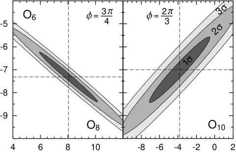
Figure 3: Confidence level contours, obtained from 2-parameter fits of the sum rule (15) in the range $M^{2}=0.4-1\,{\rm GeV}^{2}$. The condensates are in $10^{-3}\,{\rm GeV}^{D}$, the contours show $1,2,3\sigma$ deviations of $\chi^{2}$.

The condensates, obtained from real part of Borel transformation (14), are sensitive to exact value of $f_{\pi}$. For this reason we shall use the imaginary part (15) for numerical fit. The best angles are $\phi=2\pi/3,3\pi/4,4\pi/5$ where the contribution of the operators $O_{8},O_{10},O_{12}$ vanishes respectively. The fit results for each angle are summarized in the Table 1. The lowest errors are obtained from the 2-parameter fits at the first two angles. The deviation $\chi_{0}^{2}$ for these fits is sufficiently small. For this reason the inclusion of additional parameters, say $O_{12}$, will not improve the fit quality, but will increase the errors only.

The operator values, obtained from the sum rules, are not independent but have large covariances

$$\rho_{ij}=\overline{\Delta O_{i}\,\Delta O_{j}}/(\overline{(\Delta O_{i})^{2}}\,\,\overline{(\Delta O_{j})^{2}})^{1/2}.$$

All fits give $\rho_{6,10}\approx 1$ and $\rho_{6,8}\approx\rho_{8,10}\approx-1$. For the 2-parameter fits the covariances can be demonstrated on the confidence level plots, see Fig 3. The equations $\chi^{2}=n^{2}$ set the ellipses, which are the borders of the $n\sigma$ deviation area.

One may also try to fit the condensates at all these angles simultaneously by minimizing $\chi^{2}_{all}={1\over 3}[\chi^{2}(2\pi/3)+\chi^{2}(3\pi/4)+\chi^{2}(4\pi/5)]$, see the last two lines in the Table. As the final result of our analysis we take this combined fit:

$$O_{6}^{V-A} = -\,(7.2\pm 1.2)\times 10^{-3}\,{\rm GeV}^{6}$$

$$O_{8}^{V-A} = \;\;\;\,(7.8\pm 2.5)\times 10^{-3}\,{\rm GeV}^{8}$$

$$O_{10}^{V-A} = -\,(4.4\pm 2.8)\times 10^{-3}\,{\rm GeV}^{10}$$ (18)

The lower limit of the Borel mass in (16) was taken $M_{1}^{2}=0.4\,{\rm GeV}^{2}$ for the first two angles and $M_{1}^{2}=0.3\,{\rm GeV}^{2}$ for the last one. If $M_{1}^{2}$ is taken by $0.1\,{\rm GeV}^{2}$ higher, the errors are increased, especially for the high dimension operators, see the last line in the Table.

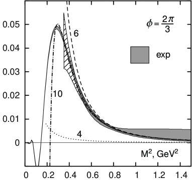
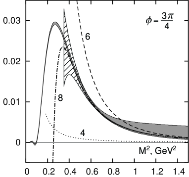
Figure 4: Imaginary part of the Borel transformation for $\phi=2\pi/3$ (no $O_{8}$) and $\phi=3\pi/4$ (no $O_{10}$). Shaded area is the l.h.s. of (15) calculated from experimental data (with error). The lines display the operator series in the r.h.s. of (15) with condensates, equal to the central values of (18). The number nearby each line shows the order of the series; say ”8” denotes the contribution $O_{4}+O_{6}+O_{8}$. Grid shows possible contribution of the operator $O_{12}$ within the limits $|O_{12}^{V-A}|<3\times 10^{-3}\,{\rm GeV}^{12}$.

The validity of our assumptions is demonstrated in the Figure 4. If the operator $O_{10}^{V-A}$ is taken into account, a good agreement of theoretical and experimental values is observed for $M^{2}>0.4\,{\rm GeV}^{2}$. Below this value the contribution of the operator $O_{12}$ could be large. Even better agreement can be found at the angles, where the operator $O_{12}$ disappears, see the plots in the Figure 5. Here the fit can be extended down to $M^{2}=0.3\,{\rm GeV}^{2}$. One may also obtain the condensates by fitting the real part of the Borel transformation (14). Here the central values of the condensates turns out to be close to (18), but the errors are higher due to the presence of additional parameter $f_{\pi}^{2}$. Combined fit of eq (14) at different angles $\phi$ gives $f_{\pi}=131\pm 4\,{\rm MeV}$. As pointed in IZ , $f_{\pi}$ itself has an ambiguity of order $m_{\pi}^{2}/m_{\rho}^{2}\sim 3\%$, the accuracy of the chiral lagrangian parameters. Notice the sign alternation in (18), in agreement with the minimal hadronic ansatz for $\Pi_{V}-\Pi_{A}$ correlator, constructed in PPR in the large $N_{c}$ limit.

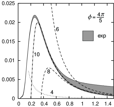
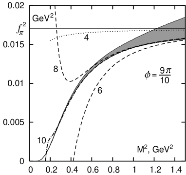
Figure 5: Imaginary part of the Borel transformation (15) at $\phi=4\pi/5$ and real part (14) at $\phi=9\pi/10$. The operator $O_{12}^{V-A}$ vanishes in these sum rules.

Finally, we write down the values of the quark condensate and the parameter $m_{0}^{2}$, obtained from the operators (18):

$$\alpha_{s}\langle{\bar{q}}q\rangle^{2}\left(1+c_{6}{\alpha_{s}\over\pi}\right)\,=\,(262\pm 9\,{\rm MeV})^{6}$$ (19)

$$m_{0}^{2}\,=\,-O_{8}^{V-A}/O_{6}^{V-A}\,=\,1.1\pm 0.2\,{\rm GeV}^{2}$$ (20)

The errors in the r.h.s. are purely experimental: they do not include possible contribution of the operator $O_{12}$ and higher as well as unknown QCD corrections to the condensates. The factor $c_{6}$ is scheme dependent and left arbitrary in (19). The accuracy of $m_{0}^{2}$ is better than accuracy of $O_{8}^{V-A}$ because of high covariance of $O_{6}$ and $O_{8}$. Notice a very good agreement of the $D=10$ condensate (18) obtained from the sum rules, with the one estimated in previous section (13) within the framework of the factorization hypothesis.

4 Conclusion

We have performed the analysis of the $V-A$ spectral functions, obtained from hadronic $\tau$-decay channels, with the help of the Borel sum rules. The values of the condensates of dimension $D=6,8,10$ were found (18) by fitting the theoretical curves of the Borel transform to the experimental ones within its errorbands. The major contribution to these condensates comes from the 4-quark operators. Its contribution to the current correlators was calculated and their size was estimated by means of the factorizations hypothesis. The estimated value of the $D=10$ condensate (13) is found to be in good agreement with the fit result (18), which demonstrates the validity of OPE approach in Quantum Chromodynamics.

Our results are based on several assumptions, in particular, the factorization (vacuum insertion) hypothesis. There is a statement in literature LNT , that factorization hypothesis underestimates the quartic condensates by a factor $\sim 3$. This conclusion is based on the comparison of the quark condensate obtained from the $D=6$ operator in $\rho$-meson (vector) sum rules with the one calculated from the low-energy GMOR theorem. (Our result (19) is also larger than GMOR condensate for reasonable theoretical parameters.) However this comparison has many other sources of error, such as scale-scheme ambiguity, high order QCD corrections, light quark masses, corrections from the chiral lagrangian etc. The accuracy of the factorization hypothesis can be of the same order as the ambiguity of the factorization of the D=8 operators the level of $O(N_{c}^{-2})$ terms, as demonstrated in IZ . More careful statement about validity of the factorization hypothesis could be obtained by evaluating the contribution of the meson states to the 4-quark condensates.

Second objection may concern rather low value of the Borel mass $M_{1}^{2}=0.4\,{\rm GeV}^{2}$ used in our fit (16). Indeed, the typical scale where perturbative results for the current correlators are confirmed, is $Q^{2}\gtrsim 1\,{\rm GeV}^{2}$. But our result for the $D=10$ operator demonstrates rather low (power-like) growth of the operators $|O_{2n+2}/O_{2n}|\sim m_{0}^{2}$ in the $V-A$ channel. If the operators grow as $|O_{2n}|\sim m_{0}^{2n}$, then the Borel series behaves as $e^{-m_{0}^{2}/M^{2}}$. The contribution of the $n+1$-term in the exponent is small for $M^{2}\gg m_{0}^{2}/n$. So for $n=5$ the minimal scale $M_{1}^{2}=0.4\,{\rm GeV}^{2}$ seems reasonable. For a faster growth of the operator series this choice could be inappropriate. For instance, if one plots the Borel transformation versus $M^{2}$ with the condensate values obtained in CGM , the divergence of the operator series will be obvious already at $M^{2}\approx 0.7\,{\rm GeV}^{2}$. However it should be mentioned, that the $D=10$ condensate obtained there exceeds our value (13) by an order of magnitude. It seems unlikely to explain such discrepancy by the inaccuracy of the factorization. All these assumptions can be confirmed or disproved only within a nonperturbative approach.

We have neglected the logarithmic terms $\sim\ln{Q^{2}}/Q^{2n}$ in the OPE series (3). Such contribution from the $\alpha_{s}$-correction to the $D=6$ condensate (5) has a small numerical factor; its discontinuity along the real axis $Q^{2}=-s<0$ is too small to compare with the spectral function $v_{1}(s)-a_{1}(s)$. For this reason it would be interesting to calculate the $\alpha_{s}^{2}$ correction to the $D=6$ $V-A$ operator and $\alpha_{s}$ correction to the operator $O_{8}^{V-A}$ and include them in the sum rule analysis.

Appendix A: 4-quark operators

The calculation of the operator contribution to various current correlators can be performed within the framework of background field method, see for instance Gr . Here we describe the algorithm, conventions and basic formulae, necessary to calculate the contribution of the 4-quark condensates to the 2-current correlator, which correspond to the third diagram of the Fig. 2. We also present here complete form of the 4-quark operators up to dimension $D=10$. For definiteness we consider only the vector current correlator; the condensate contribution to the axial current correlator is trivially obtained by the substitution $d\to\gamma^{5}d$. The contribution of the 4-quark condensates can be written as:

$$\Pi_{\mu\nu}^{V}(q)=-{ig^{2}\over 4}\int\!dx\,dy\,dz\,e^{iqx}\biggl{<}D_{\alpha\beta}^{ab}(y,z)$$ (A1)

$$\times\biggl{[}\bar{u}(x)\gamma_{\mu}S(x,y)\gamma_{\alpha}\lambda^{a}d(y)\,+\bar{u}(y)\gamma_{\alpha}\lambda^{a}S(y,x)\gamma_{\mu}d(x)\biggr{]}$$

$$\times\biggl{[}\bar{d}(0)\gamma_{\nu}S(0,z)\gamma_{\beta}\lambda^{b}u(z)\,+\bar{d}(z)\gamma_{\beta}\lambda^{b}S(z,0)\gamma_{\nu}u(0)\biggr{]}\biggr{>}$$

Here $S(x,y)=\left<Tq(x){\bar{q}}(y)\right>$ is the quark Green function and $D^{ab}_{\mu\nu}(x,y)=\left<Ta^{a}_{\mu}(x)a^{b}_{\nu}(y)\right>$ is the gluon Green function in background gluon field $A_{\mu}\to A_{\mu}+a_{\mu}$. They obey the equations:

$$i\hat{D}_{x}\,S(x,y)\,=\,i\delta^{4}(x-y)$$ (A2)

$$\left[D_{x}^{2}g_{\mu\alpha}+2G_{\mu\alpha}(x)\right]\!{}^{ac}D^{cb}_{\alpha\nu}(x,y)\,=\,i\delta^{ab}g_{\mu\nu}\delta^{4}(x-y)$$ (A3)

where $g_{\mu\nu}=(+,-,-,-)$ is Minkowski metric. The quarks are massless, the gluon Green function is taken in the Feynman gauge. The covariant derivative and the gluon field-strength tensor in the fundamental representation (A2) are defined as follows:

$$D_{\mu}=\partial_{\mu}-iA_{\mu},\quad A_{\mu}={g\over 2}\lambda^{a}A_{\mu}^{a},$$

$$G_{\mu\nu}=i[D_{\mu},D_{\nu}]={g\over 2}\lambda^{a}G^{a}_{\mu\nu}$$ (A4)

where $\lambda^{a}$ are Gell-Mann matrices ${\rm tr}(\lambda^{a}\lambda^{b})=2\delta^{ab}$, $[\lambda^{a},\lambda^{b}]$ $=if^{abc}\lambda^{c}$. We shall also use additional compact notations for these objects in adjoint representation (A3):

$$D_{\mu}^{ab}=\partial_{\mu}\delta^{ab}+A_{\mu}^{ab},\quad A_{\mu}^{ab}={g\over 2}f^{acb}A_{\mu}^{c},\quad G_{\mu\nu}^{ab}={g\over 2}f^{acb}G_{\mu\nu}^{c}$$ (A5)

It is convenient to perform partial Fourier transformation of the Green functions:

$$S(x,y) = \int\!{d^{4}q\over(2\pi)^{4}}\,e^{-iq(x-y)}{\tilde{S}}(q,y),$$

$$D^{ab}_{\mu\nu}(x,y) = \int\!{d^{4}q\over(2\pi)^{4}}\,e^{-iq(x-y)}{\tilde{D}}_{\mu\nu}^{ab}(q,y)$$ (A6)

Then one can write down the solution of equations (A2), (A3) as series in powers of background field $A$:

$$\tilde{S}(q,y) = S_{0}(q)\sum_{n=0}^{\infty}\left[i\hat{A}(\hat{x})S_{0}(q)\right]^{n},$$ (A7)

$${\tilde{D}}_{\mu\nu}^{ab}(q,y) = \Bigl{\{}D_{0}(q)\sum_{n=0}^{\infty}\left[iR(q,\hat{x})D_{0}(q)\right]^{n}\Bigr{\}}{}^{ab}_{\mu\nu},$$ (A8)

where

$$S_{0}(q)\,=\,{i\hat{q}\over q^{2}},\qquad D_{0}(q)=-{i\over q^{2}}$$

are free propagators, ${\hat{x}}=y-i\overrightarrow{\partial}$, the derivative $\overrightarrow{\partial}=\partial/\partial q$ acts on everything from the right as $[\overrightarrow{\partial}_{\mu},q_{\nu}]=g_{\mu\nu}$; $R$ is the following matrix operator:

$$R_{\mu\nu}^{ab}(q,\hat{x}) = \left[-iq_{\alpha}A_{\alpha}^{ab}(\hat{x})-iA_{\alpha}^{ab}(\hat{x})q_{\alpha}\right.$$ (A9)

$$\left.+A_{\alpha}^{ac}(\hat{x})A_{\alpha}^{cb}(\hat{x})\right]g_{\mu\nu}+2G_{\mu\nu}^{ab}(\hat{x})$$

The equations (A7), (A8) can be evaluated in a gauge covariant way in the fixed point gauge $x^{\mu}A_{\mu}(x)=0$, where

$$A_{\mu}(x) = -\int_{0}^{1}d\alpha\,\alpha x^{\nu}G_{\mu\nu}(\alpha x)$$

$$= -x^{\nu}\sum_{n=0}^{\infty}{x^{\alpha_{1}}\ldots x^{\alpha_{n}}\over(n+2)n!}\,D_{\alpha_{1}}\ldots D_{\alpha_{n}}G_{\mu\nu}(0)$$

$$q(x) = \sum_{n=0}^{\infty}{x^{\alpha_{1}}\ldots x^{\alpha_{n}}\over n!}\,D_{\alpha_{1}}\ldots D_{\alpha_{n}}q(0)$$ (A11)

In order to compute the propagators $\tilde{S}$, $\tilde{D}$ for any fixed order $n$, one has to substitute (Appendix A: 4-quark operators) into (A7), (A8), move all the derivatives $\overrightarrow{\partial}$ to the right and then leave only the terms without $\overrightarrow{\partial}$.

The 4-quark condensate contribution (A1) can be written in terms of the propagators $\tilde{S}$, $\tilde{D}$ as follows:

$$\Pi_{\mu\nu}^{V}(q) = -{ig^{2}\over 4}\biggl{[}\bar{u}(-i\overrightarrow{\partial})\gamma_{\mu}\tilde{S}(q,-i\overrightarrow{\partial})\gamma_{\alpha}\lambda^{a}d(-i\overrightarrow{\partial})\,$$ (A12)

$$\times \tilde{D}^{ab}_{\alpha\beta}(q,-i\overrightarrow{\partial})\,X^{b}_{\nu\beta}(q)+X^{b}_{\nu\beta}(q)\,\tilde{D}^{ba}_{\beta\alpha}(-q,-i\overleftarrow{\partial})$$

$$\times \bar{u}(-i\overleftarrow{\partial})\gamma_{\alpha}\lambda^{a}\tilde{S}(-q,-i\overleftarrow{\partial})\gamma_{\mu}d(-i\overleftarrow{\partial})\biggr{]},$$

where

$$X_{\nu\beta}^{b}(q) = \bar{d}(-i\overrightarrow{\partial})\gamma_{\beta}\lambda^{b}\tilde{S}(q,0)\gamma_{\nu}u(0)$$ (A13)

$$+ \bar{d}(0)\gamma_{\nu}\tilde{S}(-q,-i\overleftarrow{\partial})\gamma_{\beta}\lambda^{b}u(-i\overleftarrow{\partial})\;.$$

In the functions $\tilde{S}(q,y)$ and $\tilde{D}(q,y)$ the derivatives $\overrightarrow{\partial}$, $\overleftarrow{\partial}$ over momentum $q$ always stand on the right from any function of $q$: $\ldots q\ldots\partial$. The derivatives inside (A13) do not act on anything outside $X^{b}_{\nu\beta}$. After these derivatives are evaluated, we compute the transverse part $\Pi^{(1)}=-\Pi_{\mu\mu}/(3q^{2})$ defined according to (1). (We also checked, that longitudinal part vanishes $\Pi^{(0)}=0$.) And finally, to separate out the Lorentz invariant condensates, we average $\Pi^{(1)}$ over directions of vector $q_{\mu}$ according to:

$$\overline{q_{\mu_{1}}\ldots q_{\mu_{2n}}}=2{(2n-1)!!\over(2n+2)!!}(q^{2})^{n}g_{(\mu_{1}\mu_{2}}\ldots g_{\mu_{2n-1}\mu_{2n})},$$

$$\overline{q_{\mu_{1}}\ldots q_{\mu_{2n+1}}}=0,$$ (A14)

where $(\mu_{1}\ldots\mu_{n})$ denotes usual index symmetrization with weight $1/n!$. All these calculations were performed on computer.

The most time-consuming part of the calculation is to reduce large number of terms in the final result to minimal number of independent structures. For this purpose we employ the quark equation of motion ${\hat{D}}u={\hat{D}}d=0$ and the ”integration by part” identity $\langle A(D_{\mu}B)\rangle=-\langle(D_{\mu}A)B\rangle$ (the vacuum average of the total derivative is zero $\langle\partial_{x}O(x)\rangle=\partial_{x}\langle O(x)\rangle=\partial_{x}\langle O(0)\rangle=0$ for any gauge invariant operator $O(x)$). It allows to bring the operators to obviously hermitean (real) form, which provides an additional verification of the result.

In order to write down the 4-quark condensates in a compact form, we introduce here the following bilinear quark structures of increasing dimension $D$:

$$\begin{array}[]{ll}3D:&A_{\alpha}={\bar{d}}\lambda\gamma^{5}\gamma_{\alpha}u\\ 4D:&B^{(1)}_{\alpha\beta}=i({\bar{d}}\lambda\gamma_{\alpha}u_{\beta}-{\bar{d}}_{\beta}\lambda\gamma_{\alpha}u)\\ &B^{(2)}_{\alpha\beta}={\bar{d}}\lambda\gamma^{5}\gamma_{\alpha}u_{\beta}+{\bar{d}}_{\beta}\lambda\gamma^{5}\gamma_{\alpha}u\\ 5D:&C^{(1)}_{\alpha\beta\gamma}=i({\bar{d}}\lambda\gamma_{\alpha}u_{\beta\gamma}-{\bar{d}}_{\beta\gamma}\lambda\gamma_{\alpha}u)\\ &C^{(2)}_{\alpha\beta\gamma}={\bar{d}}\lambda\gamma^{5}\gamma_{\alpha}u_{\beta\gamma}+{\bar{d}}_{\beta\gamma}\lambda\gamma^{5}\gamma_{\alpha}u\\ &C^{(3)}_{\alpha\beta\gamma}={\bar{d}}_{\alpha}\lambda\gamma^{5}\gamma_{\beta}u_{\gamma}+{\bar{d}}_{\gamma}\lambda\gamma^{5}\gamma_{\beta}u_{\alpha}\\ &C^{(4)}_{\alpha\beta\gamma}={\bar{d}}\{\lambda,G_{\alpha\beta}\}\gamma_{\gamma}u\\ 6D:&E^{(1)}_{\alpha\beta\gamma\delta}={\bar{d}}\{\lambda,G_{\alpha\beta}\}\gamma_{\gamma}u_{\delta}+{\bar{d}}_{\delta}\{\lambda,G_{\alpha\beta}\}\gamma_{\gamma}u\\ &E^{(2)}_{\alpha\beta\gamma\delta}={\bar{d}}\{\lambda,\tilde{G}_{\alpha\beta}\}\gamma_{\gamma}u_{\delta}+{\bar{d}}_{\delta}\{\lambda,\tilde{G}_{\alpha\beta}\}\gamma_{\gamma}u\\ &E^{(3)}_{\alpha\beta\gamma\delta}=i({\bar{d}}\{\lambda,G_{\alpha\beta}\}\gamma^{5}\gamma_{\gamma}u_{\delta}-{\bar{d}}_{\delta}\{\lambda,G_{\alpha\beta}\}\gamma^{5}\gamma_{\gamma}u)\\ &E^{(4)}_{\alpha\beta\gamma\delta}=i({\bar{d}}\{\lambda,\tilde{G}_{\alpha\beta}\}\gamma^{5}\gamma_{\gamma}u_{\delta}-{\bar{d}}_{\delta}\{\lambda,\tilde{G}_{\alpha\beta}\}\gamma^{5}\gamma_{\gamma}u)\\ &E^{(5)}_{\alpha\beta\gamma\delta}={\bar{d}}\{\lambda,G_{\beta\gamma;\,\alpha}\}\gamma_{\delta}u\\ &E^{(6)}_{\alpha\beta\gamma\delta}={\bar{d}}\{\lambda,\tilde{G}_{\beta\gamma;\,\alpha}\}\gamma_{\delta}u\\ 7D:&F^{(1)}_{\alpha\beta\gamma}=i({\bar{d}}\{\lambda,J_{\alpha}\}\gamma^{5}\gamma_{\beta}u_{\gamma}-{\bar{d}}_{\gamma}\{\lambda,J_{\alpha}\}\gamma^{5}\gamma_{\beta}u)\\ &F^{(2)}_{\alpha\beta\gamma}={\bar{d}}\{\lambda,\{G_{\alpha\delta},G_{\delta\beta}\}\}\gamma^{5}\gamma_{\gamma}u\\ &F^{(3)}_{\alpha\beta\gamma}=i{\bar{d}}\{\lambda,[G_{\alpha\delta},\tilde{G}_{\delta\beta}]\}\gamma_{\gamma}u\end{array}$$ (A15)

where $u_{\alpha}=D_{\alpha}u$, $u_{\alpha\beta}=D_{(\alpha}D_{\beta)}u\equiv{1\over 2}(D_{\alpha}D_{\beta}+D_{\beta}D_{\alpha})u$, $G_{\beta\gamma;\,\alpha}=D_{\alpha}G_{\beta\gamma}$, $J_{\alpha}=D_{\beta}G_{\alpha\beta}$, $[A,B]=AB-BA$, $\{A,B\}=AB+BA$. The dual tensor is defined as $\tilde{G}_{\alpha\beta}={1\over 2}\varepsilon_{\alpha\beta\mu\nu}G_{\mu\nu}$, $\varepsilon^{0123}=1$ and $\gamma^{5}=i\gamma^{0}\gamma^{1}\gamma^{2}\gamma^{3}$. The values $G$, $\tilde{G}$, $J$ in (A15) are in fundamental representation. All bilinear structures belong to adjoint representation of the gauge group, the gauge index of the Gell-Mann matrices $\lambda$ is omitted. We denote conjugated structures by overlined letters, which are simply obtained by the replacement $u\rightleftarrows d$, for instance ${\bar{A}}_{\alpha}\equiv A_{\alpha}^{\dagger}={\bar{u}}\lambda\gamma^{5}\gamma_{\alpha}d$.

The 4-quark condensates of dimension $D=6,8,10$ are:

$$O_{6}^{V}=-2\pi\alpha_{s}\left<{\bar{A}}_{\alpha}A_{\alpha}\right>$$ (A16)

$$O_{8}^{V}={2\pi\alpha_{s}\over 9}\left<-4{\bar{B}}^{(1)}_{\alpha\beta}B^{(1)}_{\alpha\beta}-{\bar{B}}^{(2)}_{\alpha\beta}B^{(2)}_{\alpha\beta}\right.$$

$$\qquad\quad\left.-4{\bar{C}}^{(3)}_{\beta\alpha\beta}A_{\alpha}-4{\bar{A}}_{\alpha}C^{(3)}_{\beta\alpha\beta}+12{\bar{A}}_{\alpha}G_{\alpha\beta}A_{\beta}\right>$$ (A17)

$$O_{10}^{V}={\pi\alpha_{s}\over 9}\Biggl{<}25{\bar{C}}^{(1)}_{\alpha\beta\gamma}C^{(1)}_{\alpha\beta\gamma}-5{\bar{C}}^{(2)}_{\alpha\beta\gamma}C^{(2)}_{\alpha\beta\gamma}-10{\bar{C}}^{(3)}_{\alpha\beta\alpha}C^{(3)}_{\gamma\beta\gamma}$$

$$-19{\bar{C}}^{(4)}_{\alpha\beta\beta}C^{(4)}_{\alpha\gamma\gamma}-{15\over 4}{\bar{C}}^{(4)}_{\alpha\beta\gamma}C^{(4)}_{\alpha\beta\gamma}-8{\bar{C}}^{(4)}_{\alpha\beta\gamma}C^{(4)}_{\beta\gamma\alpha}$$

$$-2{\bar{B}}^{(1)}_{\alpha\beta}G_{\beta\gamma}B^{(1)}_{\alpha\gamma}-66{\bar{B}}^{(2)}_{\alpha\beta}G_{\alpha\gamma}B^{(2)}_{\gamma\beta}+{\bar{A}}_{\alpha}\Bigl{(}8J_{[\alpha;\,\beta]}$$

$$-3G_{\alpha\gamma}G_{\gamma\beta}+19G_{\beta\gamma}G_{\gamma\alpha}\Bigr{)}A_{\beta}+{33\over 4}{\bar{A}}_{\alpha}G_{\beta\gamma}G_{\beta\gamma}A_{\alpha}$$

$$+{\bar{B}}^{(1)}_{\alpha\beta}\left(E^{(1)}_{\beta\gamma\alpha\gamma}+{5\over 2}E^{(4)}_{\alpha\gamma\gamma\beta}-{7\over 2}E^{(5)}_{\gamma\beta\gamma\alpha}-28{\tilde{G}}_{\beta\gamma}B^{(2)}_{\alpha\gamma}\right.$$

$$\left.+{21\over 2}{\tilde{G}}_{\beta\gamma;\,\alpha}A_{\gamma}\right)+\left({\bar{E}}^{(1)}_{\beta\gamma\alpha\gamma}+{5\over 2}{\bar{E}}^{(4)}_{\alpha\gamma\gamma\beta}-{7\over 2}{\bar{E}}^{(5)}_{\gamma\beta\gamma\alpha}\right.$$

$$\left.+28{\bar{B}}^{(2)}_{\alpha\gamma}{\tilde{G}}_{\beta\gamma}-{21\over 2}{\bar{A}}_{\gamma}{\tilde{G}}_{\beta\gamma;\,\alpha}\right)B^{(1)}_{\alpha\beta}+{\bar{B}}^{(2)}_{\alpha\beta}\left(-{11\over 2}E^{(2)}_{\alpha\gamma\gamma\beta}\right.$$

$$\left.+{15\over 4}E^{(2)}_{\beta\gamma\alpha\gamma}+{5\over 2}E^{(3)}_{\alpha\gamma\beta\gamma}+5E^{(3)}_{\beta\gamma\alpha\gamma}+{1\over 2}E^{(6)}_{\alpha\beta\gamma\gamma}+{3\over 2}E^{(6)}_{\beta\alpha\gamma\gamma}\right.$$

$$\left.-4E^{(6)}_{\gamma\alpha\beta\gamma}-{17\over 2}G_{\alpha\beta;\,\gamma}A_{\gamma}-11J_{\beta}A_{\alpha}\right)+\left(-{11\over 2}{\bar{E}}^{(2)}_{\alpha\gamma\gamma\beta}\right.$$

$$\left.+{15\over 4}{\bar{E}}^{(2)}_{\beta\gamma\alpha\gamma}+{5\over 2}{\bar{E}}^{(3)}_{\alpha\gamma\beta\gamma}+5{\bar{E}}^{(3)}_{\beta\gamma\alpha\gamma}+{1\over 2}{\bar{E}}^{(6)}_{\alpha\beta\gamma\gamma}+{3\over 2}{\bar{E}}^{(6)}_{\beta\alpha\gamma\gamma}\right.$$

$$\left.-4{\bar{E}}^{(6)}_{\gamma\alpha\beta\gamma}+{17\over 2}{\bar{A}}_{\gamma}G_{\alpha\beta;\,\gamma}+11{\bar{A}}_{\alpha}J_{\beta}\right)B^{(2)}_{\alpha\beta}$$

$$+{\bar{A}}_{\alpha}\left(-3F^{(1)}_{\beta\alpha\beta}+F^{(1)}_{\beta\beta\alpha}+2F^{(2)}_{\alpha\beta\beta}-{1\over 2}F^{(2)}_{\beta\beta\alpha}+F^{(3)}_{(\alpha\beta)\beta}\right.$$

$$\left.-{45\over 2}{\tilde{G}}_{\alpha\beta}C^{(4)}_{\beta\gamma\gamma}+{35\over 2}{\tilde{G}}_{\beta\gamma}C^{(4)}_{\alpha\beta\gamma}+{75\over 8}{\tilde{G}}_{\beta\gamma}C^{(4)}_{\beta\gamma\alpha}\right)$$

$$+\left(-3{\bar{F}}^{(1)}_{\beta\alpha\beta}+{\bar{F}}^{(1)}_{\beta\beta\alpha}+2{\bar{F}}^{(2)}_{\alpha\beta\beta}-{1\over 2}{\bar{F}}^{(2)}_{\beta\beta\alpha}+{\bar{F}}^{(3)}_{(\alpha\beta)\beta}\right.$$

$$\left.+{45\over 2}{\bar{C}}^{(4)}_{\beta\gamma\gamma}{\tilde{G}}_{\alpha\beta}-{35\over 2}{\bar{C}}^{(4)}_{\alpha\beta\gamma}{\tilde{G}}_{\beta\gamma}-{75\over 8}{\bar{C}}^{(4)}_{\beta\gamma\alpha}{\tilde{G}}_{\beta\gamma}\right)\!A_{\alpha}\!\Biggr{>}$$

(A18)

In (A17), (A18) the field strengths $G$, $\tilde{G}$, $J$ are in adjoint representation $G_{\alpha\beta}^{ab}={g\over 2}f^{acb}G^{c}_{\alpha\beta}$ etc; gauge indices are omitted, say ${\bar{A}}_{\alpha}G_{\beta\gamma}G_{\beta\gamma}A_{\alpha}$ denotes ${\bar{A}}_{\alpha}^{a}G_{\beta\gamma}^{ab}G_{\beta\gamma}^{bc}A_{\alpha}^{c}$. The operator $O_{8}^{V}$ (A17) can be easily brought to the form, obtained in IZ and GP .

Appendix B: Factorization of 4-quark condensates

At first let us remind, how the factorization (vacuum insertion) works for the $D=6$ operators. It is illustrated by the following equation:

$$\langle({\bar{u}}\lambda\Gamma_{1}d)({\bar{d}}\lambda\Gamma_{2}u)\rangle\,=\,-2\,C_{N}\,{\rm tr}\left[\langle u\otimes{\bar{u}}\rangle\Gamma_{1}\langle d\otimes{\bar{d}}\rangle\Gamma_{2}\right]$$ (B1)

where $\Gamma_{i}$ are some Dirac matrices, $C_{N}=1-1/N_{c}^{2}$, $N_{c}$ is the color number, kept arbitrary here. In (B1) the notation $\langle q\otimes{\bar{q}}\rangle$ denotes $4\times 4$ matrix in spinor space, the color indices are contracted. It is proportional to the quark condensate:

$$\left<q\otimes{\bar{q}}\right>\,=\,-\,{1\over 4}\,\langle{\bar{q}}q\rangle$$ (B2)

The result of the factorization is well known:

$$O^{V}_{6}\,=\,-4\pi\alpha_{s}C_{N}\langle{\bar{u}}u\rangle\langle{\bar{d}}d\rangle$$ (B3)

(In the vector sum rules one also accounts additional operator $\langle{\bar{q}}\gamma_{\alpha}J_{\alpha}q\rangle$, which takes the 4-quark form when the gluon equation of motion is applied. Such operator comes from the 2-quark diagram, so it cancels in the $V-A$ correlators.)

The factorization procedure becomes ambiguous at the level of $D=8$ 4-quark condensates. As shown in IZ , different ways of factorization give different terms $\sim 1/N_{c}^{2}$. For definiteness, here we follow the following factorization scheme. At first we replace the field strength by the derivatives as $G_{\mu\nu}=i[D_{\mu},D_{\nu}]$ for fundamental representation and $G_{\mu\nu}^{ab}=[D_{\mu},D_{\nu}]^{ab}$ for adjoint one. Then we apply the equation (B1), where the quark wave functions $u,{\bar{u}}$ and $d,{\bar{d}}$ may carry some derivatives. Finally, the quark matrices $\langle\ldots\rangle$ with derivatives are expressed in terms of the condensates as:

$$\left<D_{\alpha}q\otimes{\bar{q}}\right>=0,$$

$$\left<D_{\alpha}D_{\beta}q\otimes{\bar{q}}\right>=-{1\over 32}\left(g_{\alpha\beta}+{1\over 3}\gamma_{\alpha\beta}\right)i\langle{\bar{q}}\hat{G}q\rangle,$$ (B4)

where $\gamma_{\alpha\beta}=\gamma_{[\alpha}\gamma_{\beta]}={1\over 2}(\gamma_{\alpha}\gamma_{\beta}-\gamma_{\beta}\gamma_{\alpha})$, $\hat{G}=\gamma_{\alpha\beta}G_{\alpha\beta}$. The result for the $D=8$ condensate is:

$$O_{8}^{V}\,=\,-2\pi\alpha_{s}C_{N}\left[\,\langle{\bar{u}}u\rangle\,i\langle{\bar{d}}\hat{G}d\rangle\,+\,\langle{\bar{d}}d\rangle\,i\langle{\bar{u}}\hat{G}u\rangle\,\right]$$ (B5)

In the condensate $O_{10}$ one encounters the terms with quarks carrying 4 derivatives. We average these terms with the help of the following rule:

$$\left<D_{\alpha}D_{\beta}D_{\gamma}D_{\delta}q\otimes{\bar{q}}\right>\,=\,-{1\over 24^{2}}\bigl{[}g_{\alpha\beta}g_{\gamma\delta}(3X_{2}+6X_{3}-2X_{4})$$

$$+g_{\alpha\gamma}g_{\beta\delta}(6X_{1}+3X_{2}+6X_{3}+4X_{4})+g_{\alpha\delta}g_{\beta\gamma}(12X_{1}$$

$$+3X_{2}+6X_{3}+4X_{4})+(g_{\alpha\beta}\gamma_{\gamma\delta}+g_{\gamma\delta}\gamma_{\alpha\beta})(X_{1}+2X_{2}$$

$$+3X_{3})+(g_{\alpha\gamma}\gamma_{\beta\delta}+g_{\beta\delta}\gamma_{\alpha\gamma})(2X_{1}+X_{2}+3X_{3}+X_{4})$$

$$+g_{\alpha\delta}\gamma_{\beta\gamma}(X_{1}+2X_{2}+X_{4})+g_{\beta\gamma}\gamma_{\alpha\delta}(X_{1}+X_{4})$$

$$+3\gamma_{\alpha\beta\gamma\delta}X_{2}\bigr{]}$$ (B6)

where $\gamma_{\alpha\beta\gamma\delta}=\gamma_{[\alpha}\gamma_{\beta}\gamma_{\gamma}\gamma_{\delta]}$, $X_{i}$ are 7-dimensional condensates, defined in (10).

Being applied to the operator (A18), this procedure gives the following result:

$$O_{10}^{V} = \pi\alpha_{s}C_{N}\left[\,{25\over 9}\,\langle{\bar{u}}\hat{G}u\rangle\langle{\bar{d}}\hat{G}d\rangle\ \,-\right.$$ (B7)

$$-\,4\left(3X_{1}^{u}-X_{2}^{u}+X_{3}^{u}+{7\over 6}X_{4}^{u}\right)\langle{\bar{d}}d\rangle$$

$$\left.-\,4\left(3X_{1}^{d}-X_{2}^{d}+X_{3}^{d}+{7\over 6}X_{4}^{d}\right)\langle{\bar{u}}u\rangle\,\right]$$

where $X_{i}^{q}$ are constructed from the quark of flavor $q$. The axial condensates can be obtained by simple replacement $d\to\gamma^{5}d$. For all factorized 4-quark operators $O_{D}^{A}=-O_{D}^{V}$.

References

• (1) M.A. Shifman, A.I. Vainstein, V.I. Zakharov, Nucl. Phys. B 147, 385, 448 (1979)
• (2) ALEPH collaboration: R. Barate et al, Eur. J. Phys. C 4, 409 (1998)
• (3) OPAL collaboration: K. Ackerstaff et al, Eur. J. Phys. C 7, 571 (1999)
• (4) B.L. Ioffe, K.N. Zyablyuk, Nucl. Phys. A 687, 437 (2001)
• (5) E. Braaten, S. Narison, A. Pich, Nucl. Phys. B 373, 581 (1992)
• (6) M. Davier, L. Girlanda, A. Hocker, J. Stern, Phys. Rev. D 58, 096014 (1998)
• (7) S. Peris, B. Phily, E. de Rafael, Phys. Rev. Lett. 86, 14 (2001)
• (8) J. Bijnens, E. Gamiz, J.Prades, JHEP 0110, 009 (2001)
• (9) V. Cirigliano, E. Golowich, K. Maltman, Phys. Rev. D 68, 054013 (2003)
• (10) C.A. Dominguez, A. Schilcher, Phys. Lett B 581, 193 (2004)
• (11) S. Ciulli, C. Sebu, K. Schilcher, H. Spiesberger, hep-ph/0312212
• (12) J. Rojo, J.I. Latorre, JHEP 0401, 055 (2004)
• (13) S.C. Generalis, J. Phys. G 15, L225 (1989)
• (14) K.G. Chetyrkin, S.G. Gorishny, V.P. Spiridonov, Phys. Lett. B 160, 149 (1985)
• (15) M. Gell-Mann, R.J. Oakes, B. Renner, Phys. Rev. 175, 2195 (1968)
• (16) L.V. Lanin, V.P. Spiridonov, K.G. Chetyrkin, Yad. Fiz. 44, 1372 (1986)
• (17) L.-E. Adam, K.G. Chetyrkin, Phys. lett. B 329, 129 (1994)
• (18) M.S. Dubovikov, A.V. Smilga, ITEP-82-42
• (19) A. Grozin, Y. Pinelis, Phys. Lett. B 166, 429 (1986)
• (20) V.M. Belyaev, B.L. Ioffe, Sov. Phys. JETP 56, 493 (1982)
• (21) H.G. Dosch, M. Jamin, S. Narison, Phys. Lett. B 220, 251 (1989)
• (22) S. Narison, Phys. Lett. B 210, 238 (1988)
• (23) T.-W. Chiu, T.-H. Hsieh, Nucl. Phys. B 673, 217 (2003)
• (24) A.Di Giacomo, Yu.A. Simonov, hep-ph/0404044
• (25) B.L. Ioffe, K.N. Zyablyuk, Eur. Phys. J. C 27, 229 (2003)
• (26) G. Launer, S. Narison, R. Tarrach, Z. Phys. C 26, 433 (1984)
• (27) A.G. Grozin, Int. J. Mod. Phys. A 10, 3497 (1995)