13.03.2004

WIC/07/04-MAR-DPP

A New Algorithm for Inclusive Search of SUSY Signals.

Ehud Duchovni , Eugene Prosso and Peter Renkel

Particle Physics Department,
Weizmann Institute of Science, Rehovot 76100, Israel

A new algorithm designed to reduce the model dependence in future SUSY searches at the LHC is described. This algorithm can dynamically adapt itself to a wide range of possible SUSY final states thus reducing the need for detailed model-driven analysis. Preliminary study of its performance on simulated MSSM, GMSB and AMSB final states is described, and a comparison with traditional search procedures, whenever available, is performed.

1 Introduction

While the case for nature to be supersymmetric is very appealing, the understanding of the way in which Supersymmetry is broken is far from being established. The details of this symmetry breaking determine the SUSY mass spectrum and consequently the way in which SUSY will exhibit its existence at the LHC. An attempt to perform a virtually model independent search for a large class of possible SUSY final states is reported in this note. The outlines of the proposed wide-scope algorithm are presented in the next section. The widening of the scope of the search is achieved by dynamic adaptation of the algorithm to the peculiarities of the signal. Such a procedure is likely to result in a reduction of the search sensitivity when compared to sophisticated dedicated analysis techniques like Artificial Neural Networks (ANN), which are based on a prior knowledge of the signal characteristics but the deterioration is shown to be marginal and the algorithm performs significantly better than simple cuts. It is argued that a combination of the traditional Model driven searches and the present wide scope procedure will allow ATLAS to conduct the most effective search for SUSY (and probably other) final states. These statements are substantiated by the MC studies that are described in the following sections.

2 Description of the technique

The exact nature of the expected SUSY final states depends on the details of the way SUSY is broken and is yet unknown. Be it as it may, one has some general hints for the nature of such final states:

• Very high mass: since SUSY particles must be heavy (Tevatron, LEP);

• Large missing energy: at least in all RPC models due to the existence of a neutral practically non-interacting LSP.

An attempt to construct a search procedure in the most general way possible, based on these hints, is described in this note.

2.1 The LSL algorithm

The K-neighborhood algorithm [1] was modified in such a way that it can cope with the task of finding small deviations from the simulated expectations, which might result from the presence of an unspecified signal. In the modified algorithm - the LSL (Local Spherical Likelihood) [2] - each event is described by N parameters and is represented by a point in a corresponding N-dimensional space, where the N axes correspond to the N parameters. The generic name for such a space is the ’event-space’. The choice of parameters (i.e. axes) is crucial as it determines to which type of signal the analysis will be sensitive. This is the place where model dependence is introduced into the procedure. Once the parameters (i.e. the axes) have been chosen one normalizes them (usually the parameters are mapped in such a way that they are centered at zero and distributed between zero and one) in order to remove the effect of variable scaling.

Next, one runs a simulation of all the relevant SM processes and places each of the simulated events in an event-space, which is named the ’reference’ space. One proceeds then by constructing a similar event-space using all data events, this event-space is named the ’data’ space.

The essence of the algorithm is to look for local accumulations of events in the ’data’ space, which are absent in the ’reference’ space. In the LSL, in order to expose the existence of such a local high-density region each of the data events is placed inside the ’reference’ space and an N-dimensional sphere is traced around it. The radius of this sphere is adjusted in such a way that it is the minimum that is required to contain exactly $N_{B}$ reference events, where $N_{B}$ is a predefined number. The radius of this sphere is then recorded. Next a sphere with the same radius is traced around the same data event but this time this is done in the ’data’ space and the number of data events that are contained in the sphere $N_{D}$ is determined.
In the absence of signal one expects $N_{D}\approx N_{B}$. If signal were present one would expect $N_{D}>N_{B}$ .
In order to discern the presence of signal the quantity:

$$\rho(N_{B})={N_{D}-N_{B}\over\sqrt{N}_{B}}$$

is computed. A large value of $\rho$, which is the parameter that quantifies the local deviation of the density of the data from the density of the background, is therefore, an indication for a possible existence of a signal.

The numerical value above which $\rho$ can be considered large enough to constitute an evidence for the presence of a signal in the data is not well defined at this stage. In order to estimate this value one makes use of additional SM simulated events (which are not used for the construction of the ’reference’ space) and construct a ’null’ space, namely, data-like event-space in which instead of data one places SM simulated events (without a signal). One can then repeat the procedure outlined above for the ’null’ space and get the $\rho$ distribution for the no-signal hypothesis. The actual value of $\rho$ as computed from the data, can now be compared with the null-hypothesis and acquire a meaningful statistical interpretation.

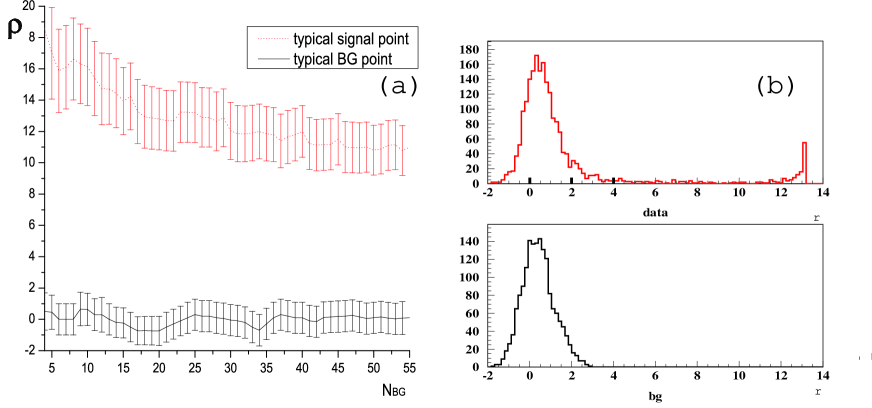
Figure 1b shows the $\rho$ (for fixed $N_{B}$ = 21) distribution for the signal case (upper red histogram) and for a background case (lower blue histogram). The peak at $\rho\approx 13$ in the signal case is an artifact of the situation in which the n-dimensional sphere is located at the center of a well separated cluster of signal events. The sphere contains all the signal in the cluster and the radius is then artificially enlarged to include the required 21 background events. Thus, the spheres around different data points inside this cluster contain the same set of background and, consequently, signal events. As a result the $\rho$ value of all the events in this cluster is roughly the same.

Figure 1: a) The variation of $\rho$ as a function of the size of the sphere ($N_{B}$) for a typical background (black line, lower band) and signal (red line, upper band) events. b) $\rho^{max}$ distribution for the signal case (upper red solid histogram) and for a simulated background, (lower black histogram). Note the long tail of high $\rho$ events in the signal plot. The small peak at large $\rho^{max}$ in the upper plot is discussed in the text.

The size of the sphere, namely the numerical value of $N_{B}$ depends on the number of simulated events as well as on the shape that the signal cloud takes inside the event space. Since the second factor is unknown the procedure is repeated for values of $N_{B}$ ranging from some minimal value $N_{0}$ (21 in the present study) to some fixed value, say 5% of the number of background events in the reference space. The maximal attainable $\rho$ in the series of $\rho(N_{B})$, is denoted by $\rho^{max}$.
As mentioned above a large value of $\rho^{max}$ is a strong indication for the existence of a signal in the data.
The variation of $\rho$ as a function of $N_{B}$ is shown in Figure  1a for typical background and signal event. Since $\rho(N_{B})$ is strongly correlated with $\rho(N_{B}-1)$ the maximum value of $\rho$ as obtained by this procedure is fairly stable. It is disadvantageous to evaluate $\rho$ at low values of $N_{B}$ since for such values the statistical error is large. It is equally disadvantageous to evaluate $\rho$ at high values of $N_{B}$ since then the radius of the sphere is large and one looses the locality nature of the analysis.

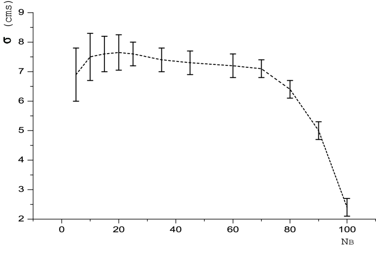
At that point one can select a fixed $N_{B}$ for which the attainable $\rho$ are large or continue with $\rho_{max}$ at the cost of having a variable $N_{B}$. The results which are presented below have been obtained using the best $\rho_{max}(N_{B})$ attainable provided $N_{B}>20$. The dependence of sensitivity of the analysis on $N_{B}$ is shown in Figure  2 for the case of GMSB with $\Lambda=170~{}TeV$, $M=1000~{}TeV$, $tan\beta=15$ and a positive $\mu$. One sees, that at small $N_{B}$ the performance is not very good because of the statistical fluctuations, while for large $N_{B}$ it decreases because of the limited number of signal events. The optimal $N_{B}$ in this case is found to be at about 60.

The whole sequence of steps is summarized in the following list:

1. Choose the parameters (motivated by physics considerations);

2. Apply a set of soft preliminary cuts (to remove irrelevant events);

3. Scale and normalize the events’ parameters;

4. Form a ’reference’ space from all relevant SM background processes;

5. Form some ’null’ space by simulating additional SM simulated events;

6. Apply the procedure that was described before, for obtaining the $\rho$ distributions to the ’reference’ space and the ’null’ space and obtain the distribution for $\rho^{max}_{null}$. The number of events in the ’null’ space should be as large as possible ;

7. Form the ’data’ space using preselected data events;

8. Apply the procedure that was described before, for obtaining the $\rho$ distributions to the ’reference’ space and ’data’ space and obtain the distribution of the data $\rho^{max}_{data}$;

9. Compute $\sigma(\rho)={N_{data}-N_{null}\over\sqrt{N_{null}}}|_{\rho>cut}$ ; where N stands for the number of events with $\rho>cut$  , and maximize this value by changing the value of $\rho_{cut}$.

Figure 2: The statistical significance of the MSSM search analysis as a function of $N_{B}$.

3 Implementation

While the algorithm which was described above can be used to search for any conceivable signal we study its performance here by applying it on various RPC SUSY simulated signals. This decision determines, as was discussed, the selection of parameters by which each event is described. On one hand one would like to have all the relevant parameters that one can think of, but on the other hand a large number of parameters will necessitates a huge number of simulated events and will make the procedure either slow or useless. Hence, only 4 input parameters, with the highest ’separation’ power, were selected. In order to conform with existing analyzes two sets are used: one in which no requirement on the presence of leptons in the event is set; and another one in which one lepton is required and its properties are included in the input parameters. The parameters for the ’no-lepton’ case were:

• $E_{t}^{miss}$ - Where $E_{t}^{miss}$ is the missing transverse energy of the event;
  

• $P_{t}^{jet_{1}}$ - Where $P_{t}^{jet_{1}}$ is the transverse momentum of the most energetic (transverse direction) jet;
  

• $P_{t}^{jet_{2}}$ - Where $P_{t}^{jet_{2}}$ is the transverse momentum of the second most energetic (transverse direction) jet;
  

• $\Sigma E_{t}$ - Where $\Sigma E_{t}$ is total transverse energy of the event.

In the case of $1-lepton$ channel the 4 input variables are:

• $E_{t}^{miss}$ - Where $E_{t}^{miss}$ is the missing transverse energy of the event;
  

• $P_{t}^{jet_{1}}$ - Where $P_{t}^{jet_{1}}$ is the transverse momentum of the most energetic (transverse direction) jet;
  

• $M_{t,l-miss}$ - Where $M_{t,l-miss}$ is the transverse mass of the lepton-missing momentum system;
  

• $\Sigma E_{t}$ - Where $\Sigma E_{t}$ is total transverse energy of the event.

The SM processes that have been simulated (using Pythia) for this study consist of the processes: $pp\rightarrow WX$; $pp\rightarrow ZX$; $pp\rightarrow t\bar{t}$; $pp\rightarrow two~{}jets$. The Equivalent luminosity was set to 10 $fb^{-1}$ and in order to keep the number of events reasonable, a $p_{t}$ cut of 200 GeV (via ckin(3) [4]) was applied. The effect of this cut was checked later and verified to be of negligible importance.

The signal was simulated using Pythia [4] (for MSSM) and ISAJET [5] (for GMSB and AMSB). The detector response was simulated using a fast simulation program . The ATLAS TDR [6] as well as some additional points were used in this study.

In order to reduce the number of background events in the various event spaces, a set of preliminary cuts was applied.

• $E_{t}^{miss}>~{}500~{}GeV$: which is due to the presence of two LSP in each event;

• $P_{t}^{jet_{1}}>200~{}GeV$: this cut and the two that follow reflect the high mass of the expected SUSY particles;

• $P_{t}^{jet_{2}}>100~{}GeV$;

• $\Sigma E_{t}>1500~{}GeV$;

• $N_{jet}>3$: this cut and the one that follows are based on the fact that SUSY events are expected to give rise to long cascade decay chains ;

• $C>0.1$, Where $C$ is the Circularity of the event.

for $1-lepton$ analysis the presence of a lepton with $p_{t}>10~{}GeV$ and $|\eta|<2.5$ allows softening some of the cuts. The preliminary cuts were therefore:

• $E_{t}^{miss}>~{}200~{}GeV$;

• $N_{jet}>3$;

• $P_{t}^{jet_{1}}>100~{}GeV$;

• $P_{t}^{jet_{2}}>50~{}GeV$;

• $\Sigma E_{t}>200~{}GeV$;

• $M_{t,l-miss}>80~{}GeV$: this cut removes most of the $W+jet$ background.

Since the main goal of the present study is the investigation of the performance of the LSL algorithm no attempt to look for optimal preselection cuts was done. Rather, the quantities that were used in [8] are used.

4 Results

The sensitivity of ATLAS to predicted signals of several RPC SUSY models was estimated using the LSL algorithm. In the case of MSSM and AMSB, it was possible to compare the LSL sensitivity to conventional procedure. Recently, a comprehensive evaluation of ATLAS’s sensitivity to a MSSM signal was performed [8]. On top of introducing a new channel, namely, the missing energy channel with no requirement on leptons, which proved to be the best search channel, this study also introduced a sophisticated automatic cut optimization procedure which is based on the Simplex algorithm. Figure  3 is a comparison between this technique in which the signal is simulated and cuts are optimized in numerous points and the LSL algorithm in which no simulation of the signal was used at all.

Figure 3: The sensitivity reach of ATLAS to MSSM signal in the missing energy channel with no requirements set on the number of leptons in the event. The solid (black) line is from  [8] and the dashed (red) one is the result of the LSL algorithm.

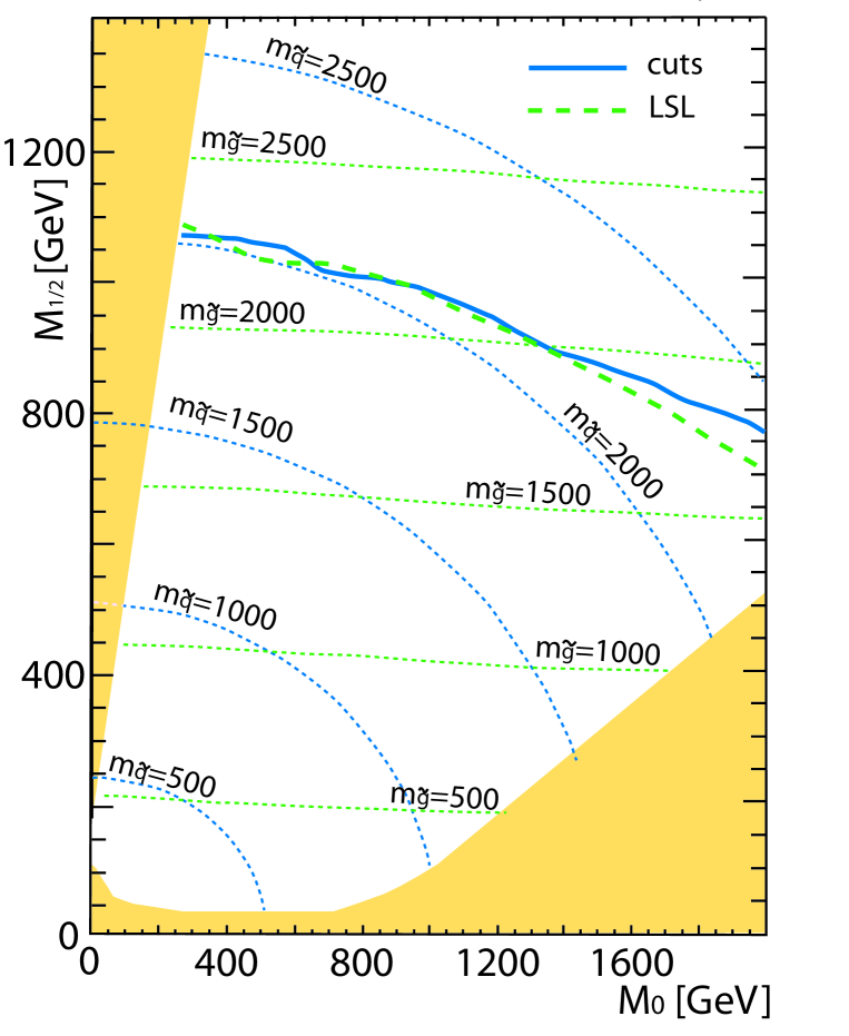
Figure  4a is a similar comparison between the two methods when only events with no leptons are considered. A somewhat complementary case, namely the case when events are required to have one isolated energetic lepton is shown in Figure  4b. An attempt to combine these two searches was also carried out. Such a combination, which is similar to the one applied in Higgs boson searches at LEP, is expected to lead to an improved sensitivity. However, the improvement which was obtained was only marginal.

Figure 4: The sensitivity reach of ATLAS to MSSM signal in the missing energy channel with no leptons in the event (a) and with one leptons in the event (b). The solid (black) line is from  [8] and the dashed (red) one is the result of the LSL algorithm.

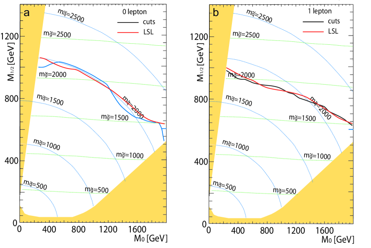
Generally speaking one may conclude from these plots that the sensitivity of the two methods is comparable. Yet one should bare in mind that the LSL algorithm did not make any use of simulated signal. For completeness sake the sensitivity of ATLAS for a MSSM signal as estimated with the LSL algorithm for luminosities of 1, 10 and 100 $fb^{-1}$ is presented in Figure 5.

Figure 5: The sensitivity reach of ATLAS to MSSM signal as estimated using the LSL algorithm for luminosities of 1, 10 and 100 $fb^{-1}$ .

A Study of ATLAS sensitivity to possible AMSB signal was carried out by Barr, Allanach, Lester and Parker [9]. In order to extract a signal a set of quantities were selected and were subjected to various cuts. 10 sets of such cuts were used for the various analyzes that have been done: 0-lepton, 1-lepton, 2-oppositely charged lepton etc.. In order to compare the LSL performance with this analysis while keeping the wide-scope approach, the null and reference spaces that were used in the MSSM case were used also here. No modification whatsoever was introduced except for the introduction of a simulated AMSB signal into the data space instead of the MSSM one. The comparison of the $E_{miss}$ analyzes is shown in figure 6.

Figure 6: A comparison between the LSL sensitivity and the published results [9] of the search for AMSB signal. The blue circled area represents the estimated sensitivity of the dedicated search while the thick dotted black line is the LSL sensitivity limit.

The two analyzes are again comparable except for the right side of Figure 6 where the LSL performance is inferior to the conventional technique. This behavior is related to the number of events with large number of jets and the differences in their simulation between Herwig (used by [9]) and Pythia (background simulation in LSL case). Note that the sensitivity region here is estimated by ${S\over\sqrt{B}}>5$ and $S>10$.

For completeness a three-luminosity contour, with 1, 10 and 100 $fb^{-1}$ is also given when the sensitivity is estimated with a more stable estimator, namely requiring ${S\over\sqrt{S+B}}>5$ where S and B are the number of signal and background events respectively.

Figure 7: The sensitivity reach of ATLAS in the AMSB parameter space for luminosities of 1, 10 and 100 $fb^{-1}$.

A similar procedure was repeated for the GMSB case. The LSL inputs were left unchanged and the estimated ATLAS sensitivity is shown in Figure  8. It is found again to be comparable to the one which was obtain with a naive set of conventional cuts  [10].

The LSL is basically looking for deviations of the data from the SM expectation, as predicted by the simulation. As such it might be sensitive to the quality of the simulation. Defects in the simulation can easily be misinterpreted as indication of a signal. Some preliminary studies of the stability of the algorithm under artificial distortion of the simulation are described in Appendix A.

Figure 8: Sensitivity reach of ATLAS for GMSB signal.

5 Conclusion

The LSL sensitivity was shown to be comparable to the one attainable by carefully adjusting the cuts to a signal of well-known characteristics. It is possible that a more sophisticated analysis, which is based on likelihood or artificial neural networks, will be superior to the LSL algorithm. Yet one should bare in mind that the LSL algorithm did not make any use of simulated signal. Hence, the LSL will be able to observe signals of unpredicted nature and once such deviation are exposed; they will be studied using all available analysis tools.

6 Acknowledgments

We would like to thank the members of the Weizmann group: Eilam Gross, Arie Melamed-Katz, Michael Riveline and Lidija Zivkovic for their help in discussing the various aspect of the present work. We would also like to thank Dan Tovey for his help in making this paper clearer. We are obliged to the Benoziyo center for High Energy Physics for their support of this work. This work was also supported by the Israeli Science Foundation(ISF) and by the Federal Ministry of Education, Science, Research and Technology (BMBF) within the framework of the German-Israeli Project Cooperation in Future-Oriented Topics(DIP).

Appendix A

Differences between the data and the simulated signals trigger the LSL algorithm. Such differences may indicate the presence of a signal but might result also from bad modelling of the detector and/or from bad modelling of the various SM processes. In order to evaluate the effect of the later sources few preliminary studies have been done. The first test checked the sensitivity to energy calibration. The energy of the ’measured’ events (i.e. those in the data space) was scaled down by 5% while that of the simulated SM (the reference space) was left untouched. The efficiency/purity of the signal selection procedure for a MSSM signal under these conditions was compared to the one which was obtained under normal conditions. The results are shown in Figure 9a

Figure 9: The efficiency vs. purity curve under normal conditions and after scaling down the jet energy in the ’data’ by 5%.

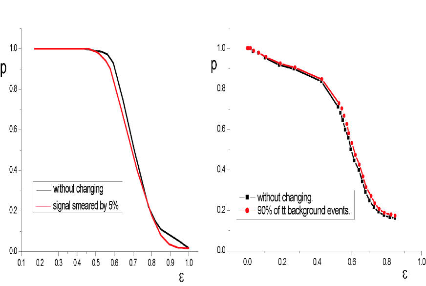
Another potential source of fake signal is mismodelling of SM processes. In order to evaluate the importance of this source of trouble the $t\bar{t}$ process was scaled down by 10% in the reference space, leaving the ’data’ richer in $t\bar{t}$ by 10% more that ’predicted. The efficiency vs purity performance curve of the LSL is shown in Figure 9b.

One may conclude from these two tests that the algorithm is fairly stable to the tested forms of distortion.

References

- [1] T. Hastie and R. Tibshirani, IEEE PAMI, 18 607-616, 1996.
- [2] E. Prosso, MSc. Thesis, Weizmann Istitute of Science, July 2002.
- [3] B. Knuteson HEP-EX/0105027, 0006011.
- [4] Pythia 6.2 Physics and Manual.Torbjorn Sjostrand, Leif Lonnblad, Stefen Mrenna, Peter Scands LU-TP 01-21 (2002).
- [5] ISAJET 7.63 A Monte-Carlo Event Generator, Frank E. Paige and Serban D. Protopescu.
- [6] ATLAS Detector and Physics Performans TDR, CERN LHCC/99-14 vol II.
- [7] T. Hastie and R. Tibshirani, IEEE PAMI, 18, 607-616, 1996.
- [8] D.R. Tovey, ’Inclusive SUSY Searches and Measurements at ATLAS’, Eur. Phys. J. C4(2002) N4, SN-ATLAS-2002-020.
-
[9]
Discovering anomaly-mediated supersymmetry at the
LHC
Barr, A J; Allanach, Benjamin C; Lester, C G; Parker, M A; Richardson, Peter.
hep-ph/0210182, J. High Energy Phys. 03 (2003) 045 - [10] E. Duchovni, ATLAS Physics Workshop, Lund, September 2001.