Abstract

We briefly illustrate the impact of the genuinely weak one-loop virtual terms of the ${\cal O}(\alpha_{\rm S}\alpha_{\rm EW}^{3})$ factorisable corrections to the three-jet cross section at $\sqrt{s}=M_{Z}$. Their importance for the measurement of $\alpha_{\rm S}$ at GigaZ luminosities is emphasised.

1 Three-jets events at leptonic colliders

In the case of $e^{+}e^{-}$ annihilations, the most important QCD quantity to be extracted from multi-jet events is $\alpha_{\mathrm{S}}$. The confrontation of the measured value of the strong coupling constant with that predicted by the theory through the renormalisation group evolution is an important test of the Standard Model (SM) or else an indication of new physics, when its typical mass scale is larger than the collider energy, but which can manifest itself through virtual effects. Not only jet rates, but also jet shape observables, which offer a handle on non-perturbative QCD effects via large power corrections, would be affected.

We report here on the calculation of the one-loop weak-interaction corrections to three-jet observables in electron-positron annihilations through the order ${\cal O}(\alpha_{\rm S}\alpha_{\rm EW}^{3})$ generated via the interference of the graphs in Fig. 1 with the tree-level ones for $\gamma^{*},Z\to\bar{q}qg$ final states, where the external $\gamma^{*},Z$ current is intended to connect to an incoming $e^{+}e^{-}$ fermion line. In the figure, the shaded blob represents all the contributions to the gauge boson self-energy and is dependent on the Higgs mass (we have set $M_{H}=115$ GeV for the latter). We neglect, however, loops involving the Higgs boson coupling to the fermion lines. The graphs in which the exchanged gauge boson is a $W$-boson are accompanied by those in which the latter is replaced by its corresponding Goldstone boson. There is then a similar set of diagrams in which the direction of the fermion line is reversed, with the exception of the last graph, as here reversal does not lead to a distinct topology. Corrections along the $e^{+}e^{-}$ lines are also included in our analysis. In short, we compute the factorisable effects only, i.e., corrections to the initial and final states only. Whereas these should be sufficient to describe adequately the phenomenology of three-jet events at $\sqrt{s}=M_{Z}$, at energy scales much larger than the $Z$-boson mass one expects comparable effects due to the non-factorisable corrections, in which weak gauge-bosons connect via one-loop diagrams electrons and positrons to quarks and antiquarks, whose computation is currently in progress.

We will show that such factorisable corrections are of a few percent at $\sqrt{s}=M_{Z}$. Hence, while their impact is not dramatic in the context of LEP1 and SLC, where the total error on the measured value of $\alpha_{\mathrm{S}}$ is larger, at a future Linear Collider (LC) [1], running at the $Z$ mass peak (e.g., GigaZ), they ought to be taken into account in the experimental fits, as here the uncertainty on the value of the strong coupling constant is expected to be at the $0.1\%$ level or even smaller [2]. The calculation has been performed using helicity amplitudes so that it can be applied to the case of polarised beams, option that is one of the strengths of the LC projects. Besides, another aspect that should be recalled is that weak corrections naturally introduce parity-violating effects in jet observables, detectable through asymmetries in the cross-section, which are often regarded as an indication of physics beyond the SM. Comparison of theoretical predictions involving parity-violation with future LC experimental data is regarded as another powerful tool for confirming or disproving the existence of some beyond the SM scenarios, such as those involving right-handed weak currents and/or new massive gauge bosons.

2 Calculation

For the techniques used in the calculation of the one-loop diagrams in Fig. 1, as well as for the relevant SM input parameters, we refer the reader to  [3].

The three-parton cross section for $e^{+}e^{-}\to\bar{q}qg$ can be written in terms of nine form-factors [4, 5]. The latter generate the doubly differential cross-section for three-jet production in terms of some event shape variable, $S$, which is in turn related to the energy fractions $x_{1},\,x_{2}$ of the antiquark and quark, respectively ($x_{i}=\frac{2E_{i}}{\sqrt{s}}$), by some function, $s$, i.e., $S=s(x_{1},x_{2})$, and of the polar and azimuthal angles, $\alpha,\,\beta$, between, e.g., the incoming electron beam and the antiquark jet:

$$\frac{d^{3}\sigma}{dS\,d\cos\alpha\,d\beta} = \int dx_{1}dx_{2}~{}\delta\left(S-s(x_{1},x_{2})\right)\left[(2-\sin^{2}\alpha)\,F_{1}+(1-3\cos^{2}\alpha)\,F_{2}\right.$$ (1)

$$\hskip 28.45274pt+\,\lambda_{e}\,\cos\alpha\,F_{3}+\sin 2\alpha\cos\beta\,F_{4}+\sin^{2}\alpha\cos 2\beta\,F_{5}+\lambda_{e}\,\sin\alpha\cos\beta\,F_{6}$$

$$\hskip 28.45274pt+\,\sin 2\alpha\sin\beta\,F_{7}+\sin^{2}\alpha\sin 2\beta\,F_{8}\left.+\,\lambda_{e}\,\sin\alpha\sin\beta\,F_{9}\right].$$

The last three terms ($F_{7},...F_{9}$) arise for the first time at the one-loop level, since they are proportional to the imaginary parts of the helicity-matrix. $F_{3},\ F_{6}$ and $F_{7}$ vanish in the parity-conserving limit and can therefore be used as probes of weak interaction contributions to three-jet production. Moreover, $F_{3}$ and $F_{6}$ would be exactly zero at tree level if the leading order process were only mediated by virtual photons. Finally, notice that upon integrating over the antiquark angle relative to the electron beam, only the form-factor $F_{1}$ survives. (The expression of the nine form-factors in terms of the helicity amplitudes can be found in Ref. [3].)

In general, it is not possible to distinguish between quark, antiquark and gluon jets, although the above expression can easily be adapted such that the angles $\alpha,\beta$ refer to the leading jet. However, (anti)quark jets can be recognised when they originate from primary $b$-(anti)quarks, thanks to rather efficient flavour tagging techniques (such as $\mu$-vertex devices). We will therefore consider the numerical results for such a case separately.

3 Numerical results

The processes considered here are the following:

$$e^{+}e^{-}\to\gamma^{*},Z\to\bar{q}qg\quad{\mathrm{(all~{}flavours)}},$$ (2)

when no assumption is made on the flavour content of the final state, so that a summation will be performed over $q=d,u,c,s,b$-quarks, and

$$e^{+}e^{-}\to\gamma^{*},Z\to\bar{b}bg,$$ (3)

limited to the case of bottom quarks only in the final state. All quarks in the final state of (2)–(3) are taken as massless. In contrast, the top quark entering the loops in both reactions has been assumed to be massive. We can systematically neglect higher order effects from Electro-Magnetic (EM) radiation without incurring into gauge-invariance violations. We do not include beamstrahlung corrections either.

It is common in the specialised literature to define the $n$-jet fraction $R_{n}(y)$ as

$$R_{n}(y)=\frac{\sigma_{n}(y)}{\sigma_{0}},$$ (4)

where $y$ is a suitable variable quantifying the space-time separation among hadronic objects and with $\sigma_{0}$ identifying the (energy-dependent) Born cross-section for $e^{+}e^{-}\to\bar{q}q$. For the choice $\mu=\sqrt{s}$ of the renormalisation scale, one can conveniently write the three-jet fraction in the following form:

$$R_{3}(y)=\left(\frac{\alpha_{\mathrm{S}}}{2\pi}\right)A(y)+\left(\frac{\alpha_{\mathrm{S}}}{2\pi}\right)^{2}B(y)+...,$$ (5)

where the coupling constant $\alpha_{\mathrm{S}}$ and the functions $A(y)$ and $B(y)$ are defined in the $\overline{\mbox{MS}}$ scheme. An experimental fit of the $R_{n}(y)$ jet fractions to the corresponding theoretical prediction is a powerful way of determining $\alpha_{\mathrm{S}}$ from multi-jet rates. Leading-order (LO) terms enter $A(y)$ while next-to-leading order QCD effects (hereafter, labelled as NLO-QCD) are embedded in $B(y)$, see [8], with contribution from both (genuine) three- and (unresolved) four-parton final states. The weak corrections of interest (hereafter, labelled as NLO-W) only contribute to the former. Hence, in order to account for these, it suffices to make the replacement

$$A(y)\to A(y)+A_{\mathrm{W}}(y)$$ (6)

in eq. (5). The jet multiplicity of the hadronic final state is determined through the implementation of so-called ‘jet clustering algorithms’ (see [9] for a description of their properties). Among the latter we use the JADE (J) [10], Durham (D) [11], Cambridge (C) [12] and Geneva (G) [13] ones.

Fig. 2 displays the $A(y)$, $-A_{\rm{W}}(y)$ and $B(y)$ coefficients entering eqs. (5)–(6), as a function of $y$ (a jet separation parameter [9]) for the above four jet algorithms at $\sqrt{s}=M_{Z}$. (Notice that $A(y)$ and $A_{\rm{W}}(y)$ for the C scheme are identical to those for the D one.) A comparison between $A(y)$ and $A_{\rm{W}}(y)$ reveals that the NLO-W corrections are negative and remain at the percent level, i.e., of order $\frac{\alpha_{\rm EM}}{2\pi s_{W}^{2}}$. They give rise to corrections to $\sigma_{3}(y)$ of –1%, and thus are generally much smaller than the NLO-QCD ones. In this context, no systematic difference is seen with respect to the choice of jet clustering algorithm, over the typical range of application of the latter at $\sqrt{s}=M_{Z}$ (say, $y_{\mathrm{cut}}\>\raisebox{-2.15277pt}{$\stackrel{{\scriptstyle\textstyle>}}{{\sim}}$}\>0.005$ for D, C and $y_{\mathrm{cut}}\>\raisebox{-2.15277pt}{$\stackrel{{\scriptstyle\textstyle>}}{{\sim}}$}\>0.01$ for G, J).

As already mentioned, it should now be recalled that jets originating from $b$-quarks can efficiently be distinguished from light-quark jets. Besides, the $b$-quark component of the full three-jet sample is the only one sensitive to $t$-quark loops, hence one may expect somewhat different effects from weak corrections to process (3) than to (2) (the residual dependence on the $Z\bar{q}q$ couplings is also different). This is confirmed by Fig. 3, where we present the total cross section at $\sqrt{s}=M_{Z}$ for $e^{+}e^{-}\to\gamma^{*},Z\to\bar{b}bg$ as obtained at LO and NLO-W, for our usual choice of jet clustering algorithms and separations. A close inspection of the plots reveals that NLO-W effects can reach the $-2.0\%$ level or so.

In view of these percent effects being well above the error estimate expected at a future high-luminosity LC running at the $Z$ pole, it is then worthwhile to further consider the effects of NLO-W corrections to some other ‘infrared-safe’ jet observables typically used in the determination of $\alpha_{\mathrm{S}}$, the so-called ‘shape variables’. A representative quantity in this respect is the Thrust (T) distribution [15]. This is defined as the sum of the longitudinal momenta relative to the (Thrust) axis $n_{\rm T}$ chosen to maximise this sum, i.e.:

$$\mbox{T}={\rm max}\frac{\sum_{i}|\vec{p_{i}}\cdot\vec{n_{\mathrm{T}}}|}{\sum_{i}|\vec{p_{i}}|},$$ (7)

where $i$ runs over all final state objects. This quantity is identically one at Born level, getting the first non-trivial contribution through ${\cal O}(\alpha_{\mathrm{S}}\alpha_{\rm EW}^{2})$ from events of the type (2)–(3). Also notice that any other higher order contribution will affect this observable. Through ${\cal O}(\alpha_{\mathrm{S}}^{2}\alpha_{\rm EW}^{2})$, for the choice $\mu=\sqrt{s}$ of the renormalisation scale, the T distribution can be parametrised in the following form:

$$(1-{\rm{T}})\frac{d\sigma}{d\mbox{T}}\frac{1}{\sigma_{0}}=\left(\frac{\alpha_{\mathrm{S}}}{2\pi}\right)A^{\mathrm{\tiny T}}(\mbox{T})+\left(\frac{\alpha_{\mathrm{S}}}{2\pi}\right)^{2}B^{\mathrm{\tiny T}}(\mbox{T}).$$ (8)

Again, the replacement

$$A^{\mathrm{\tiny T}}(\mbox{T})\to A^{\mathrm{\tiny T}}(\mbox{T})+A^{\mathrm{\tiny T}}_{\rm{W}}(\mbox{T})$$ (9)

accounts for the inclusion of the NLO-W contributions.

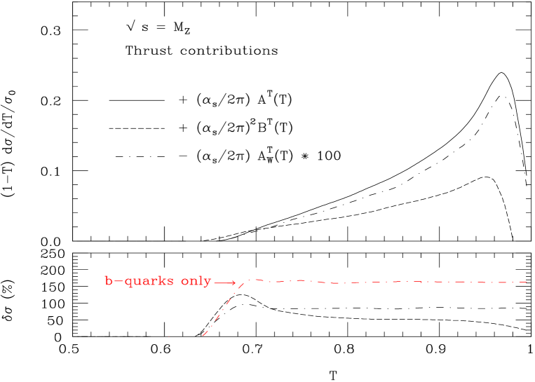
Figure 4: The LO, NLO-QCD and NLO-W contributions to the coefficient functions entering the integrated Thrust distribution, see eq. (8), for process (2) (top) and the relative size of the two NLO corrections (bottom), at $\sqrt{s}=M_{Z}$. The correction for the case of $b$-quarks only is also presented, relative to the LO results for process (3). (Notice that the $A_{\mathrm{W}}$ terms have been plotted with opposite sign and multiplied by hundred for better presentation.)

We plot the terms $\left(\frac{\alpha_{\mathrm{S}}}{2\pi}\right)A^{\mathrm{\tiny T}}(\mbox{T})$, $\left(\frac{\alpha_{\mathrm{S}}}{2\pi}\right)A^{\mathrm{\tiny T}}_{\rm{W}}(\mbox{T})$ and $\left(\frac{\alpha_{\mathrm{S}}}{2\pi}\right)^{2}B^{\mathrm{\tiny T}}(\mbox{T})$ in Fig. 4, always at $\sqrt{s}=M_{Z}$, alongside the relative rates of the NLO-QCD and NLO-W terms with respect to the LO contribution. Here, it can be seen that the NLO-W effects can reach the level of $-1\%$ or so and that they are fairly constant for $0.7\>\raisebox{-2.15277pt}{$\stackrel{{\scriptstyle\textstyle<}}{{\sim}}$}\>{\rm{T}}\>\raisebox{-2.15277pt}{$\stackrel{{\scriptstyle\textstyle<}}{{\sim}}$}\>1$. For the case of $b$-quarks only, similarly to what seen already for the inclusive rates, the NLO-W corrections are larger, as they can reach the $-1.6\%$ level.

The ability to polarise electron (and possibly, positron) beams joined with the high luminosity available render future LCs a privileged environment in which to test the structure of hadronic samples. As noted earlier, differential spectra may well carry the distinctive hallmark of some new and heavy strongly interactive particles (such as squarks and gluinos in Supersymmetry), whose rest mass is too large for these to be produced in pairs as real states but that may enter as virtual objects into multi-jet events. Similar effects may however also be induced by the NLO-W corrections tackled here. Observables where such effects would immediately be evident are the so-called the ‘unintegrated’ (or ‘oriented’) Thrust distributions associated to each of the form-factors in eq. (1) (wherein $S={\rm T}$), as can be seen in Fig. 7 of Ref. [3]. Here, as a benchmark for future studies along the above lines, we directly reproduce in Figs. 5–6 the differential structure of the nine form-factors given in eq. (1), as a function of the energy fractions $x_{1}$ and $x_{2}$, at $\sqrt{s}=M_{Z}$ (at this energy, the shape is basically the same for both final states in (2)–(3)), for the case of a left- and right-handed incoming electrons, respectively. Here, we should mention that the NLO-W corrections to the corresponding non-zero tree-level distributions were found of the order $-$(1–2)% on average for the case of the unflavoured sample and twice as much for the case of the $b$-quark one, with the corrections arising almost entirely from the left-handed incoming electrons. Finally notice that all nine distributions in Figs. 5–6, in the presence of a precise determination of $\alpha$ and $\beta$ (or, for that matter, any other combination of angles used to parametrise the event orientation), are directly observable in the case the $\bar{b}bg$ final state if also the charge (other than the flavour) of the quark is known, e.g., via high-$p_{T}$ lepton tagging from $B$-meson decays or via global jet charge determination. If not, all distributions in Figs. 5–6 have to be symmetrised around the $x_{1}=x_{2}$ direction. In the case of the full hadronic sample $\bar{q}qg$, when no flavour tagging is available, one normally identifies the two most energetic jets in the three-jet sample with those originating from the quark-antiquark pair. Although not always true, this approach is known to be a good approximation for most studies (see, e.g., Ref. [16]). Hence, even in this case one may be able to verify to a good approximation the shape of the form-factors $F_{1},...F_{9}$ in terms of the energy fractions.

4 Summary

In conclusion, we have found that, at $\sqrt{s}=M_{Z}$, the size of the NLO-W corrections to three-jet rates and event shapes is rather small, of order percent or so, hence confirming that determinations of $\alpha_{\mathrm{S}}$ at LEP1 and SLC are stable in this respect and that the SM background to parity-violating effects possibly induced by new physics is well under control. In contrast, NLO-W effects ought to be included in the case of future high-luminosity LCs running at the $Z$ pole, such as GigaZ, where the accuracy of $\alpha_{\mathrm{S}}$ measurements from such observables is expected to reach the $0.1\%$ level. Effects from NLO-W corrections are somewhat larger in the case of $b$-quarks in the final state, in comparison to the case in which all flavours are included in the hadronic sample, because of the presence of the top quark in the one-loop virtual contributions.

Since the exploitation of beam polarisation effects will be a key feature of experimental analyses of hadronic events at future LCs, we have computed the full differential structure of three-jet processes in the presence of polarised electrons and positrons, in terms of the energy fractions of the two leading jets and of two angles describing the final state orientation. The cross-sections were then parametrised by means of nine independent form-factors, the latter presented as a function of the (anti)quark energy fractions. Three of these form-factors carry parity-violating effects which cannot then receive contributions from ordinary QCD. For the two that are non-zero at LO, i.e., $F_{3}$ and $F_{6}$, the NLO-W corrections were found as large as $4\%$, for the case of $b$-quarks. Such higher-order weak effects should appropriately be subtracted from hadronic samples in the search for physics beyond the SM.

Figure 1: Graphs describing $\gamma^{*},Z\to\bar{q}qg$ in presence of one-loop weak corrections.

Figure 2: The $A(y)$, $-A_{\mathrm{W}}$ and $B(y)$ coefficient functions of eqs. (5)–(6) for the Cambridge, Durham, Geneva and Jade jet clustering algorithms, at $\sqrt{s}=M_{Z}$. (Notice that the $A_{\mathrm{W}}$ term has been plotted with opposite sign for better presentation.)

Figure 3: The total cross section for process (3) at LO and NLO-W for the Cambridge, Durham, Geneva and Jade jet clustering algorithms, at $\sqrt{s}=M_{Z}$. (Notice that the NLO-W results have been plotted with opposite sign for better presentation.)

$-F_{1}$

$x_{2}$         $x_{1}$

$-F_{2}$

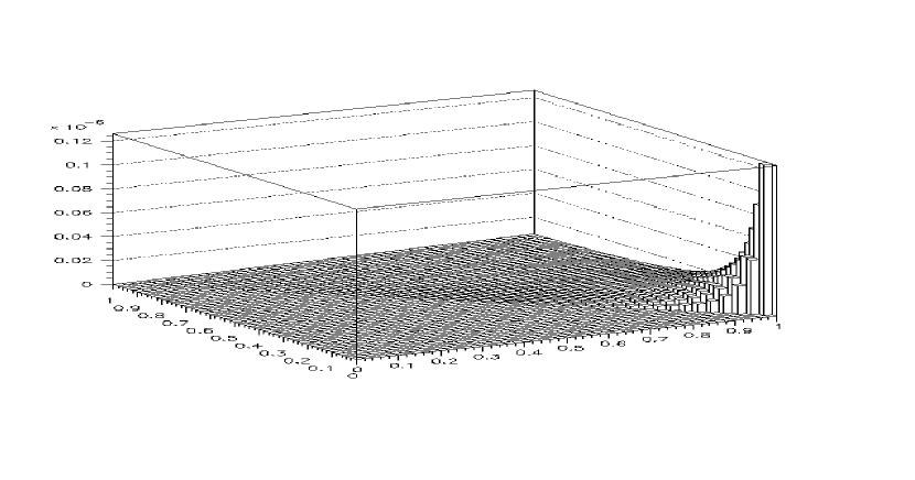
$x_{2}$         $x_{1}$

$+F_{3}$

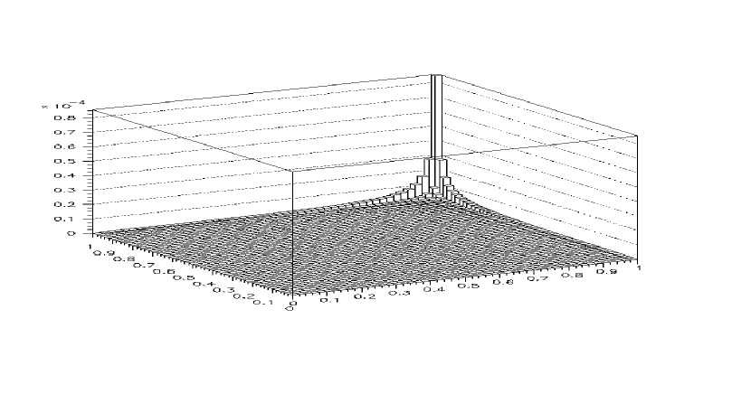
$x_{2}$         $x_{1}$

$+F_{4}$

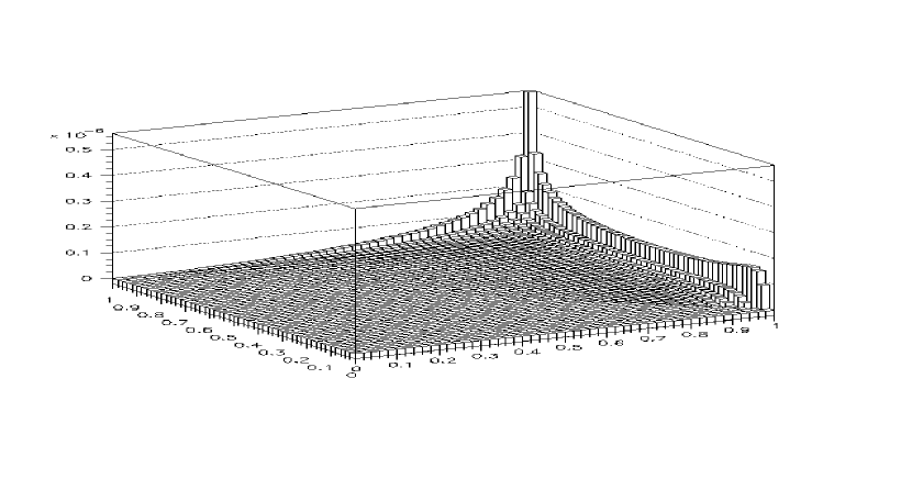
$x_{2}$         $x_{1}$

$-F_{5}$

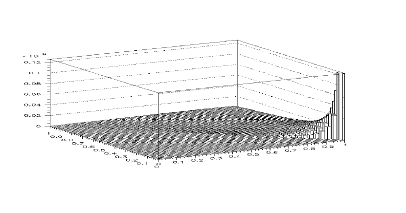
$x_{2}$         $x_{1}$

$-F_{6}$

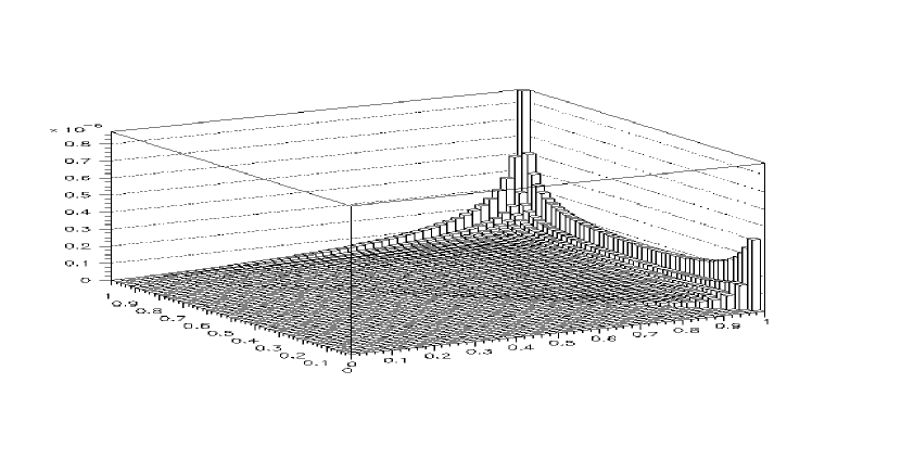
$x_{2}$         $x_{1}$

$-F_{7}$

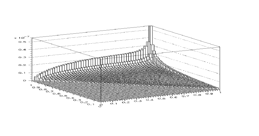
$x_{2}$         $x_{1}$

$-F_{8}$

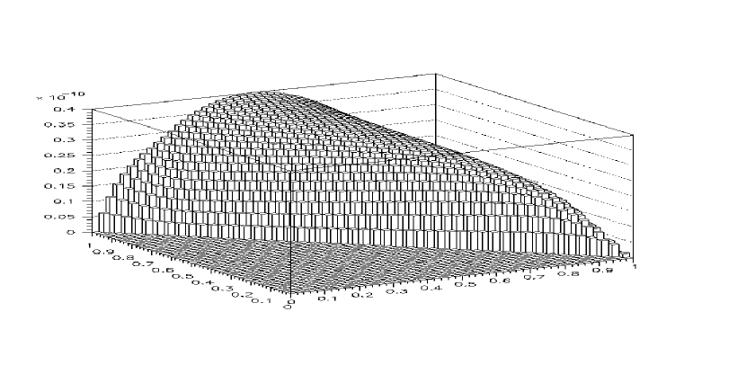
$x_{2}$         $x_{1}$

$-F_{9}$

$x_{2}$         $x_{1}$

Figure 5: The nine form-factors defined in eq. (1) as a function of the antiquark ($i=1$) and quark ($i=2$) energy fractions $x_{i}=\frac{2E_{i}}{\sqrt{s}}$ at $\sqrt{s}=M_{Z}$ in units of nb, for left-handed incoming electrons. (Note that in some cases we plot the opposite of the form-factor.)

$-F_{1}$

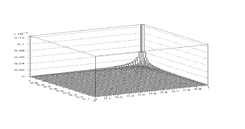
$x_{2}$         $x_{1}$

$-F_{2}$

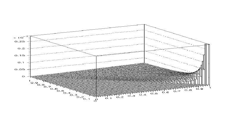
$x_{2}$         $x_{1}$

$-F_{3}$

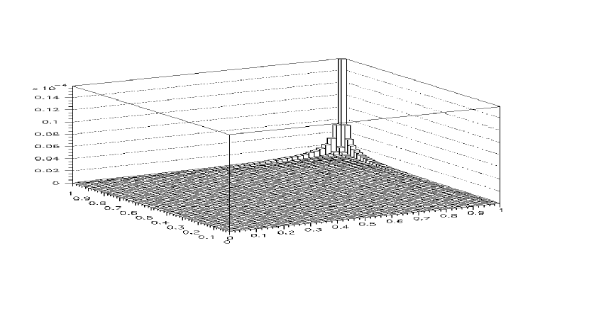
$x_{2}$         $x_{1}$

$+F_{4}$

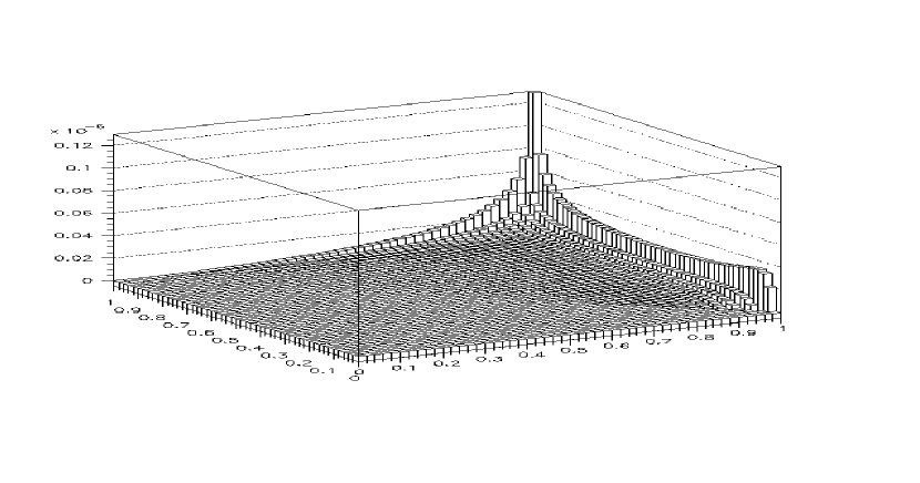
$x_{2}$         $x_{1}$

$+F_{5}$

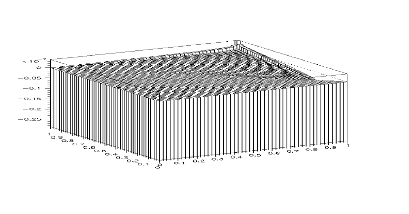
$x_{2}$         $x_{1}$

$+F_{6}$

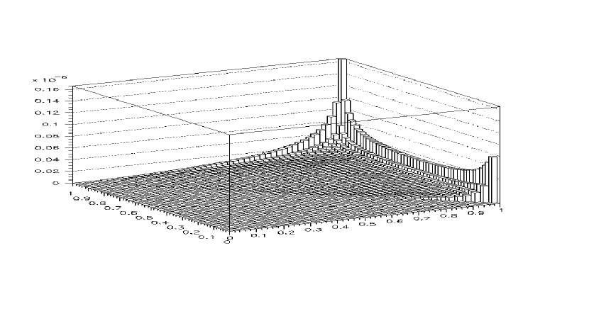
$x_{2}$         $x_{1}$

$-F_{7}$

$x_{2}$         $x_{1}$

$-F_{8}$

$x_{2}$         $x_{1}$

$+F_{9}$

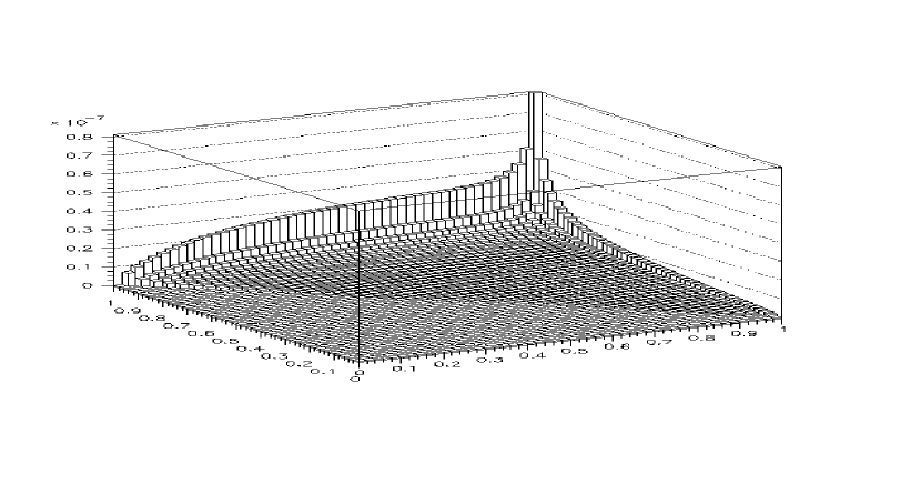
$x_{2}$         $x_{1}$

Figure 6: The nine form-factors defined in eq. (1) as a function of the antiquark ($i=1$) and quark ($i=2$) energy fractions $x_{i}=\frac{2E_{i}}{\sqrt{s}}$ at $\sqrt{s}=M_{Z}$ in units of nb, for right-handed incoming electrons. (Note that in some cases we plot the opposite of the form-factor.)

References

- [1] K. Abe et al., [The ACFA Linear Collider Working Group], hep-ph/0109166; T. Abe et al., [The American Linear Collider Working Group], hep-ex/0106055; hep-ex/0106056; hep-ex/0106057; hep-ex/0106058; J.A. Aguilar-Saavedra et al., [The ECFA/DESY LC Physics Working Group], hep-ph/0106315; G. Guignard (editor), [The CLIC Study Team], preprint CERN-2000-008 (2000).
- [2] M. Winter, LC Note LC-PHSM-2001-016, February 2001 (and references therein).
- [3] E. Maina, S. Moretti and D. A. Ross, JHEP 04 (2003) 056.
- [4] A. Brandenburg, L. Dixon and Y. Shadmi, Phys. Rev. D53 (1996) 1264.
- [5] J.G. Körner and G. Schuler, Z. Phys. C26 (1985) 559; K. Hagiwara, T. Kuruma and Y. Yamada, Nucl. Phys. B358 (1991) 80.
- [6] A. Ballestrero, E. Maina and S. Moretti, Phys. Lett. B294 (1992) 425; Nucl. Phys. B415 (1994) 265.
-
[7]
G. Rodrigo, A. Santamaria and M. Bilenky,
Phys. Rev. Lett. 79 (1997) 193;
J. Phys. G25 (1999) 1593;
hep-ph/9802359;
G. Rodrigo, hep-ph/9703359; Nucl. Phys. Proc. Suppl. 54A (1997) 60;
W. Bernreuther, A. Brandenburg and P. Uwer, Phys. Rev. Lett. 79 (1997) 189;
A. Brandenburg and P. Uwer, Nucl. Phys. B515 (1998) 279;
P. Nason and C. Oleari, Phys. Lett. B407 (1997) 57; Nucl. Phys. B521 (1998) 237. - [8] R.K. Ellis, D.A. Ross and A.E. Terrano, Nucl. Phys. B178 (1981) 421.
- [9] S. Moretti, L. Lönnblad and T. Sjöstrand, JHEP 08 (1998) 001.
-
[10]
JADE Collaboration, Z. Phys. C33 (1986) 23;
S. Bethke, Habilitation thesis, preprint LBL 50-208 (1987). -
[11]
Yu.L. Dokshitzer, contribution cited in the ‘Report of the
Hard QCD Working Group’, in
Proceedings of the workshop ‘Jet Studies at LEP and HERA’,
Durham, December 1990, J. Phys G17 (1991) 1537;
S. Catani, Yu.L. Dokshitzer, M. Olsson, G. Turnock and B.R. Webber, Phys. Lett. B269 (1991) 432. - [12] Yu.L. Dokshitzer, G.D. Leder, S. Moretti and B.R. Webber, JHEP 08 (1997) 001.
- [13] S. Bethke, Z. Kunszt, D.E. Soper and W.J. Stirling, Nucl. Phys. B370 (1992) 310; Erratum, hep-ph/9803267.
- [14] F.A. Berends, W.T. Giele and H. Kuijf, Nucl. Phys. B321 (1989) 595; W.T. Giele and E.W.N. Glover, Phys. Rev. D46 (1992) 1980.
- [15] E. Fahri, Phys. Rev. Lett. 39 (1977) 1587.
- [16] See, e.g.: T. Hebbeker, Phys. Rep. 217 (1992) 69 (and references therein).