Jet Azimuthal Correlations and Parton Saturation
in the Color Glass Condensate

Abstract

We consider the influence of parton saturation in the Color Glass Condensate on the back-to-back azimuthal correlations of high $p_{T}$ hadrons in $pA$ (or $dA$) collisions. When both near–side and away–side hadrons are detected at mid-rapidity at RHIC energy, the effects of parton saturation are constrained to transverse momenta below the saturation scale $p_{T}\leq Q_{s}$; in this case the back-to-back correlations do not disappear but exhibit broadening. However when near-side and away-side hadrons are separated by several units of rapidity, quantum evolution effects lead to the depletion of back-to-back correlations as a function of rapidity interval between the detected hadrons (at fixed $p_{T}$). This applies to both $pp$ and $pA$ (or $dA$) collisions; however, due to the initial conditions provided by the Color Glass Condensate, the depletion of the back-to-back correlations is significantly stronger in the $pA$ case. An experimental study of this effect would thus help to clarify the origin of the high $p_{T}$ hadron suppression at forward rapidities observed recently at RHIC.

Recently, a strong suppression of the high $p_{T}$ hadron yields has been observed at forward rapidities at RHIC RHICres1 ; RHICres2 ; RHICres3 ; RHICres4 . Since this effect has been predicted KLM ; KKT ; Alb ; BKW as a signature of quantum evolution in the Color Glass Condensate GLR ; hdQCD ; MV ; IF , the observations have excited considerable interest. In this paper we consider an observable which allows to test further the origin of the observed effect – the azimuthal back-to-back correlations of high $p_{T}$ hadrons. To do this, we extend the KLMN approach KN ; KL ; KLN ; KLM ; KLNDA , that has been developed to describe the experimental data on hadron multiplicities and the inclusive high $p_{T}$ yields, to the azimuthal correlations RHICAZ .

The azimuthal correlations provide a powerful method for the diagnostics of a partonic system (for a recent treatment of azimuthal correlations in nuclear collisions, see KT ). As we will show in this paper, the measurements of the strength of back-to-back correlations allow one to tell whether the partonic system under study has reached the density needed for the formation of Color Glass Condensate (CGC), or whether it is still in the perturbative QCD (pQCD) phase. Indeed, in leading order pQCD a typical hard scattering process at high energy is composed of a gluon jet with a large transverse momentum ($p_{1,t}$) balanced in the opposite direction by another gluon jet with transverse momentum ($p_{2,t}$) which is also large and almost compensates the value of $p_{1,t}$, namely, $\vec{p}_{2,t}-\vec{p}_{1,t}\,\,=\,\,\vec{q}_{1}+\vec{q}_{2}\,\ll\,\,|p_{1,t}|$ ( see Fig. 1). However, in the CGC phase of QCD the phenomenon of saturation implies a different structure of the event: a jet with large transverse momentum can be compensated by the production of several gluons with the average transverse momenta which are about equal to the saturation scale ($Q_{s}$) ($p_{2,t}\,\approx\,Q_{s}$).

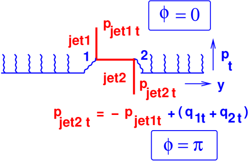
Figure 1: Back-to-back correlations of produced jets in the perturbative phase based on the QCD factorization.

In the transitional region dominated by quantum evolution (“Color Quantum Fluid” phase or region of extended scaling), the dynamics is driven by the interplay of these two mechanisms, which we are now going to discuss in more detail.

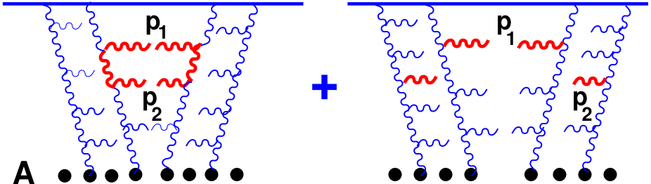
Figure 2: Two mechanisms of double inclusive production.

The first one is the production of two gluon jets from one parton shower (see the first diagram of Fig. 2) while the second mechanism is the production of two jets from different parton showers (see the second diagram of Fig. 2).

Due to AGK cutting rules AGK , the contribution of the one parton shower production to the double inclusive is described by one Mueller diagram of Fig. 3-a.

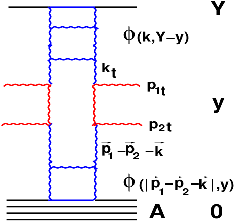
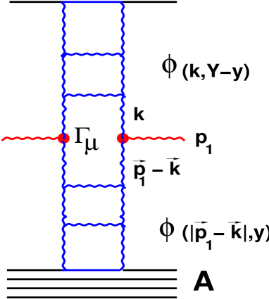
Fig. 3-a	Fig. 3-b

Figure 3: Double inclusive cross section for two correlated jet production in the perturbative phase of QCD (Fig. 3-a) and single inclusive cross section for a single jet production (Fig. 3-b).

The vertex of the gluon emission $\Gamma_{\mu}$ in Fig. 3-b (so-called Lipatov vertex) is equal to (see for example Ref. GLR )

$$\Gamma_{\mu}\,\,=\,\,\,\frac{2\,g}{p^{2}_{1t}}\,\left(p^{2}_{1,t}\,k_{\mu}\,\,-\,k^{2}_{t}\,p_{1,\mu}\,\right)$$ (1)

which leads to

$$\Gamma_{\mu}\,\Gamma^{\mu}\,\,=\,\,4\,\alpha_{S}\,\frac{k^{2}_{t}\,(\vec{p}_{1,t}-\vec{k}_{t})^{2}}{p^{2}_{1,t}}$$ (2)

Taking these equations into account one can see that the double inclusive cross section given by the diagram of Fig. 3-a is equal to (see Fig. 3-a) (see Ref.IF for details)

$$\frac{1}{\sigma}\,\frac{d^{2}\sigma}{dy_{1}\,dy_{2}\,d^{2}p_{1,t}\,d^{2}p_{2,t}}\,\,=$$

$$=\left(\frac{4N_{c}\,\alpha_{S}}{N^{2}-1}\right)^{2}\,\,\frac{1}{p^{2}_{1,t}\,\,p^{2}_{2,t}}\,\,\int\,\,d^{2}\,k_{t}\,\varphi_{projectile}(k^{2}_{t},Y-y_{1})\,\,\varphi_{target}(|\vec{p}_{1,t}-\vec{p}_{2,t}-\vec{k}_{t}|,y_{2})$$

$$=\,\,\left(\frac{4N_{c}\,\alpha_{S}}{N^{2}-1}\right)^{2}\,\,\frac{1}{p^{2}_{1,t}\,\,p^{2}_{2,t}}\,\,F^{INCL}(|\vec{p}_{1,t}-\vec{p}_{2,t}|,Y-y_{1},y_{2})\,\,$$ (3)

It should be stressed that the single inclusive cross section of Fig. 3-b can be rewritten through the same function $F^{INCL}$, namely

$$\frac{1}{\sigma}\,\frac{d\sigma}{dy\,\,d^{2}p_{1,t}}\,\,=\,\,\left(\frac{4N_{c}\,\alpha_{S}}{N^{2}-1}\right)\int\,\,d^{2}\,k_{t}\,\varphi_{projectile}(k^{2}_{t},Y-y)\,\,\varphi_{target}(|\vec{p}_{1,t}-\vec{k}_{t}|,y)$$

$$=\,\,\left(\frac{4N_{c}\,\alpha_{S}}{N^{2}-1}\right)\,\,\frac{1}{p^{2}_{1,t}}\,\,F^{INCL}(p_{1,t},Y-y,y)\,\,$$ (4)

The production of jets from two different parton showers which is described by the second diagram in Fig. 2 can be calculated using the Mueller diagram of Fig. 4. It is easy to understand that this diagram gives the double inclusive cross section in the factorized form

$$\frac{1}{\sigma}\,\frac{d^{2}\sigma}{dy_{1}\,dy_{2}\,d^{2}p_{1,t}\,d^{2}p_{2,t}}\,\,=\,\,\,\frac{1}{\sigma}\,\frac{d\sigma}{dy_{1}\,\,d^{2}p_{1,t}}\,\times\,\frac{1}{\sigma}\,\frac{d\sigma}{dy_{2}\,\,d^{2}p_{2,t}}$$ (5)

corresponding to the independent (uncorrelated ) production of two gluons with kinematic variables $(y_{1},p_{1,t})$ and $(y_{2},p_{2,t})$.

Let us now define the correlation function in the azimuthal angle $\phi$ between the two gluons as a probability to find a second gluon with rapidity $y_{2}$ and transverse momentum $p_{2,t}$ moving at the angle $\phi$ with respect to the trigger gluon with rapidity $y_{1}$ and transverse momentum $p_{1,t}$. Defined this way correlation function has the following form:

$$R(\phi;p_{1},p_{2},y_{1}=y_{2})\,\,=$$ (6)

$$\frac{F^{INCL}(|\vec{p}_{1,t}-\vec{p}_{2,t}|,Y-y_{1},y_{2})\,\,+\,\,F^{INCL}(p_{1,t},Y-y_{1},y_{1})\,\,F^{INCL}(p_{2,t},Y-y_{2},y_{2})}{\int\,\,d\,\phi\,\left(F^{INCL}(|\vec{p}_{1,t}-\vec{p}_{2,t}|,Y-y_{1},y_{2})\,\,+\,\,F^{INCL}(p_{1,t},Y-y_{1},y_{1})\,\,F^{INCL}(p_{2,t},Y-y_{2},y_{2})\right)}.$$

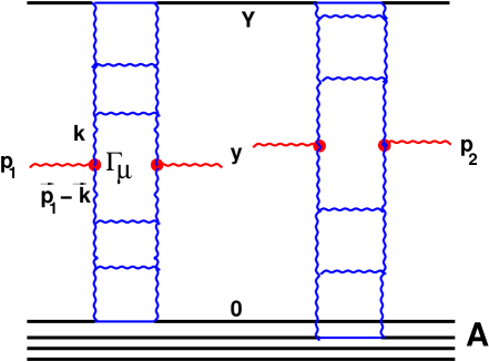
Figure 4: The Mueller diagram for the production of two gluon jets from different parton showers.

The azimuthal angle dependence originates only from the production of two gluon jets from the same parton shower (see Eq. (3)) while the second mechanism (see the secoond diagram in Fig. 2) leads to the constant background (see Eq. (5)).

The shape of the differential cross sections Eq. (3) and Eq. (5) depends crucially on the unintegrated gluon densities $\varphi$. Here we will use a simple model for these functions adopted earlier in Ref. KL :

$$\varphi(x;p^{2}_{t})\,\,=\,\,\left\{\begin{array}[]{l}\,\,\,\,\frac{\kappa}{\alpha_{S}(Q^{2}_{s})}\,S\,\,(1\,-\,x)^{4}\,\,\,\,p_{t}\,<\,Q_{s}(x)\,\,;\\ \\ \,\,\,\,\frac{\kappa}{\alpha_{S}(Q^{2}_{s})}\,S\,\frac{Q^{2}_{s}(x)}{p^{2}_{t}}\,\,(1\,-\,x)^{4}\,\,\,\,p_{t}\,>\,Q_{s}(x)\,\,;\end{array}\right.$$ (7)

In Eq. (7) we neglect, for the time being, the anomalous dimension of the gluon densities and use a very simplified assumption about the behavior of $\varphi$ reflecting the fact that inside the saturation region the density is large and changes slowly MV1 . The numerical factor $\kappa$ can be found from RHIC data on ion-ion collisions, but the value of $R$ (see Eq. (6)) does not depend on it. We introduce, as before KN ; KL ; KLN ; KLM ; KLNDA , the factor $(1\,-\,x)^{4}$ which describes that the gluon density is power suppressed at $x\,\rightarrow\,1$ according to the quark counting rules. However if we restrict ourselves to calculation of the correlation function at $y_{1}=y_{2}=0$ then the influence of these factors is very small. In general, one can expect this ansatz for $\varphi$ of Eq. (7) to be a rather crude model but it turns out to be quite successful in describing the data on rapidity and transverse momentum distributions SZC . Therefore, we hope that our calculations will provide a reasonable guideline for the experimental measurements.

For the numerical estimate we take the value of saturation scale $Q^{2}_{s}(A;y=0)=2.44\,GeV^{2}$ for gold at W=200 GeV and $Q^{2}_{s}(p;y=0)=0.26\,GeV^{2}$ for the proton in accord with our multiplicity calculations for deuteron - gold collisions KLNDA . The result is plotted in Fig. 5.

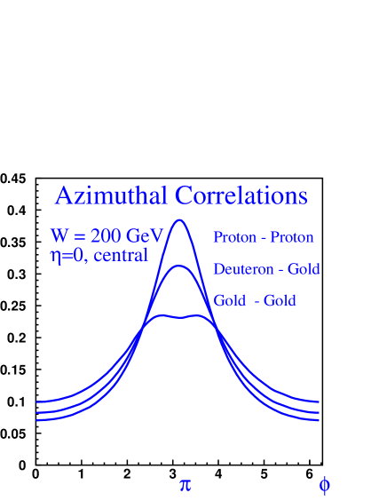
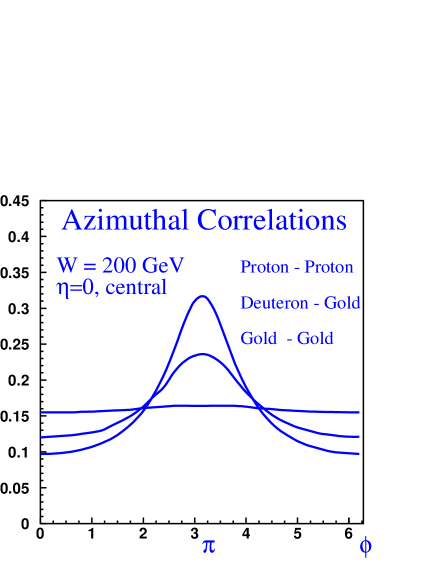
Fig. 5-a	Fig. 5-b

Figure 5: Fig. 5-a : Two gluon jet production in one parton shower normalized in a such way that the integral over azimuthal angle is equal to 1. The upper curve corresponds to proton-proton interaction, the middle one describes the deuteron-gold interaction while the third curve is related to gold-gold interaction. The calculation is performed for two jets with $p_{1}=4\,GeV$ and $p_{2}=2\,GeV$ which corresponds to STAR experiment measurements STAR . Fig. 5-b: Same as in Fig. 5-a, but for the sum of one and two parton showers.

One can see that the azimuthal angle distribution has a maximum at $\phi=\pi$ which corresponds to the jet produced in the opposite direction to the trigger jet. The width of the angular distribution is different for $pp$ and $dA$ processes. Introducing the Gaussian distribution

$$R=\frac{1}{\sqrt{2\,\pi}\sigma}\,\,e^{-\frac{(\phi-\pi)^{2}}{2\,\sigma^{2}}}$$ (8)

with the width $\sigma$, we can see from Fig. 5 that for proton-proton collision $\sigma\,=\,0.7$ while for deuteron-gold interaction $\sigma\,=\,0.8$. Therefore, the difference between the $pp$ and $dA$ processes at mid-rapidity appears quite small. However, for gold-gold interactions the $\phi$ distribution in Fig. 5 appears quite different from the Gaussian given by Eq. (8). If fitted to the Gaussian form, the value of $\sigma$ appears approximately $\sigma=1.0\div 1.2$; however this does not characterize well the distribution. This result is easy to understand qualitatively, since for large $p_{1}$ and $p_{2}$ (so large that $|p_{1}-p_{2}|\,>Q_{S}(A)$ ) the integral over $k$ in Eq. (3) stems from the region where $k\,\approx\,Q_{s}(p)<|p_{1}-p_{2}|$ and

$$F^{INCL}(|\vec{p}_{1,t}-\vec{p}_{2,t}|,Y-y_{1},y_{2})\,\,\propto\,\,\frac{Q^{2}_{s}(A)}{(p_{1}-p_{2})^{2}\,+\,2p_{1}\,p_{2}\,cos\phi}\,\,\approx\,\,\frac{\frac{Q^{2}_{s}(A)}{(p_{1}-p_{2})^{2}}}{1+\frac{2p_{1}\,p_{2}}{(p_{1}-p_{2})^{2}}\,\frac{(\phi-\pi)^{2}}{2}}$$ (9)

In this formula the typical width of the azimuthal angle distribution is equal to $\sigma_{typical}\,=\,(p_{1}-p_{2})^{2}/2\,p_{1}\,p_{2}$. For the kinematics used in the STAR experiment STAR , $p_{1}=4\,GeV$ and $p_{2}=2\,GeV$, we obtain $\sigma_{typical}\,\approx 0.5$ from this simple formula. As was mentioned above, the fact that Fig. 5 leads to a large value of $\sigma_{typical}$ is due to the region of integration over $k\approx Q_{s}(A)$.

In Fig. 5-b we plot $R(\phi;p_{1},p_{2},y_{1}=y_{2})$ for $p_{1}=4\,GeV$ and $p_{2}=2\,GeV$ as a function of $\phi$. $R$ has a meaning of the probability to find a particle with momentum $p_{2}$ at a definite angle $\phi$ if a trigger particle has a momentum $p_{1}$. The curves in this figure are quite different from Fig. 5 due to the background from the production of gluon jets from two parton showers. This background is proportional to $N_{part}^{2}$ where $N_{part}$ is the number of participants (see Refs. KL ; KLM ). In fact, this background becomes so large for gold-gold collision that we cannot see the azimuthal correlations. However, for proton - proton and deutron-gold collisions the background is not so large and we see a clear peak at $\phi=\pi$.

However, experimentalists in their analysis sometimes substract the flat background – the ”pedestal” STAR . Doing such a subtraction for Fig. 5-b and normalizing the $\phi$ - distribution to the unit area we arrive at the $\phi$ correlation functions shown in Fig. 6. It should be stressed that the ratio of the areas is equal to pp/pA= 1.16. Thus one can see that we get quite similar $\phi$ - distributions for proton-proton collisions and for deuteron-gold ones, in (at least qualitative) agreement with the data STAR .

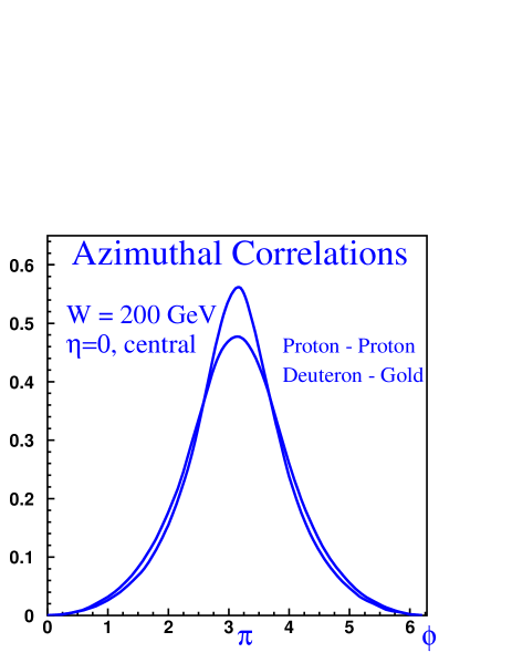
Figure 6: The azimuthal angle correlations after substraction of the background. The upper curve corresponds to proton-proton interaction while the lower one describes the deuteron-gold interaction. The calculation is performed for two jets with $p_{1}=4\,GeV$ and $p_{2}=2\,GeV$ which corresponds to STAR experiment measurements STAR

To make the main features of our approach even more transparent, let us use the following simple model for the unintegrated structure function $\varphi$ which allows us to make all calculations analytically:

$$\varphi(x;p^{2}_{t})\,\,=\,\,\frac{\kappa\,S}{\alpha_{S}(Q^{2}_{s})}\,(1-x)^{4}\,\frac{Q^{2}_{s}}{p^{2}_{t}\,+\,Q^{2}_{s}}$$ (10)

One can see that for $p_{t}\,\ll\,Q_{s}$ and for $p_{t}\,\gg\,Q_{s}$ we have the function $\varphi$ of Eq. (7) , while in the region of $p_{t}\,\approx Q_{s}$ $\varphi$ of Eq. (10) is different. The advantage of Eq. (10) is the fact that we can calculate $F^{INCL}$ of Eq. (3) and Eq. (4) analytically. Indeed, introducing Feynman parameters and taking integral over $k_{t}$ in Eq. (3) and Eq. (4) we obtain

$$F^{INCL}(p_{t},Q_{s},q_{s})\,\, = \,\,\pi\,\int^{1}_{0}\,dt\,\frac{1}{t\,(1-t)\,p^{2}_{t}\,\,+\,\,t\,(Q^{2}_{s}-q^{2}_{s})\,\,+\,\,q^{2}_{s}}\,\,$$

$$= \,\,\frac{\pi}{2\,h(p_{t},Q_{s},q_{s}}\,\,\ln\left(\frac{p^{2}_{t}\,+\,Q^{2}_{s}\,+\,q^{2}_{s}\,+\,h(p_{t},Q_{s},q_{s})}{p^{2}_{t}\,+\,Q^{2}_{s}\,+\,q^{2}_{s}\,-\,h(p_{t},Q_{s},q_{s})}\right)$$

where $Q_{s}$ and $q_{s}$ are saturation momenta of projectile and target and

$$h(p_{t},Q_{s},q_{s})\,\,=\,\,\sqrt{(p^{2}_{t}+(Q_{s}-q_{s})^{2}\,(p^{2}_{t}+(Q_{s}+q_{s})^{2}}$$ (12)

One can see that the two scales governing the azimuthal angle dependence emerge:

$$\sigma^{(-)}_{typical}\,\,=\,\frac{(p_{1}-p_{2})^{2}+(Q_{s}-q_{s})^{2}}{2\,p_{1}\,p_{2}}\,\,;\,\,\,\,\,\,\,\,\,\,\,\,\sigma^{(+)}_{typical}\,\,=\,\frac{(p_{1}-p_{2})^{2}+(Q_{s}+q_{s})^{2}}{2\,p_{1}\,p_{2}}\,\,;$$ (13)

In the case of ion-ion collisions the value of $\sigma^{(+)}_{typical}$ is rather large, and this leads to a wide distribution in $\phi$. Using this simple model, we recalculate the results presented in Fig. 5, Fig. 5-b and Fig. 6 using Eq. (Jet Azimuthal Correlations and Parton Saturation in the Color Glass Condensate); the results are presented in Fig. 7, Fig. 7-b and Fig. 8.

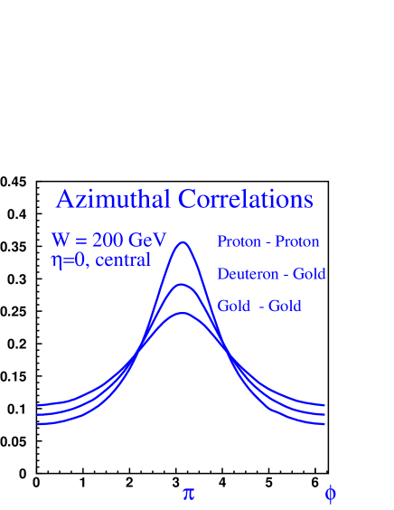
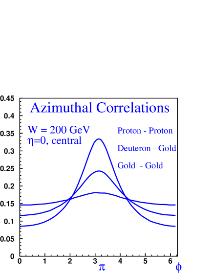
Fig. 7-a	Fig. 7-b

Figure 7: Fig. 7-a: Two gluon jet production calculated in the simple model (see Eq. (Jet Azimuthal Correlations and Parton Saturation in the Color Glass Condensate)) for the unintegrated stricture function $\varphi$ given by Eq. (10) in one parton shower normalized in a such way that the integral over azimuthal angle is equal to 1. The upper curve corresponds to proton-proton interaction, the middle one describes the deuteron-gold interaction while the third curve is related to gold-gold interaction. The calculation is performed for two jets with $p_{1}=4\,GeV$ and $p_{2}=2\,GeV$ which corresponds to STAR experiment measurements STAR . Fig. 7-b: Two gluon jet production, calculated using Eq. (Jet Azimuthal Correlations and Parton Saturation in the Color Glass Condensate), in one and in two parton showers normalized in a such way that the integral over azimuthal angle is equal to 1.

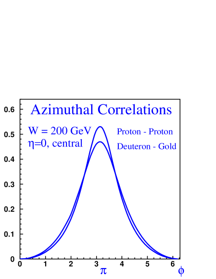
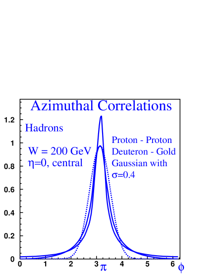
Fig. 8-a	Fig. 8-b

Figure 8: Fig. 8-a: The azimuthal angle correlations, calculated using Eq. (Jet Azimuthal Correlations and Parton Saturation in the Color Glass Condensate), after subtraction of the background. The upper curve corresponds to proton-proton interaction while the lower one describes the deuteron-gold interaction. The calculation is performed for two jets with $p_{1}=4\,GeV$ and $p_{2}=2\,GeV$ which corresponds to STAR experiment measurements STAR Fig. 8-b: The azimuthal angle correlations of produced hadrons after substraction of the background. The upper curve corresponds to proton-proton interaction while the lower one describes the deuteron-gold interaction. The calculation is performed for two jets with $p_{1}=4\,GeV$ and $p_{2}=2\,GeV$ which corresponds to STAR experiment measurements STAR . The dotted line is the Gaussian distribution of Eq. (8) with $\sigma=04$. Fragmentation is included as described in the text.

Examination of these results leads us to the conclusion that our approach explains, at least on a qualitative level, two of the most striking experimental facts: (i) the strong suppression of the azimuthal back-to-back correlations in gold-gold collisions and (ii) the close similarity of these correlations for the proton-proton and deuteron-gold interactions. (The final-state interactions of the jets in ion-ion collisions are expected to broaden the observed azimuthal correlations even more.)

It is interesting to see if we can reproduce the measured widths of the $\phi$-diastribution quantitatively. As one can see from Fig. 6, the calculated width is larger than the experimental one. One obvious reason which can contribute to this difference is the fragmentation of the jets: indeed, we have computed the correlation function for gluons, not for the measured hadrons. As a result of fragmentation, the fall-off of the inclusive cross section (and also of $F^{INCL}$ in Eq. (3) and Eq. (5)) with the transverse momentum becomes more steep. To take account of this, we use the fragmentation function of gluon jet to hadrons from Ref. KKP . One can see that the resulting width of the distribution in Fig. 8-b is indeed much smaller than in Fig. 6, and is now close to the experimental one. One can also see that the real distribution is not quite Gaussian.

One of the possibilities to check the validity of our approach is to measure the azimuthal correlations in the kinematics when both of the detected hadrons are measured at forward rapidity. Since the nuclear saturation momentum increases with rapidity, $Q_{s}(A,y)=Q_{s}(A,y=0)\,\exp[\lambda\,y]$ with $\lambda\,\approx\,0.25\,\div\,0.3$ GW , we expect a wider distribution in the azimuthal angle, than at $y=0$. Fig. 9 shows our prediction for deuteron-gold and proton - proton scattering for $y=3.8$.

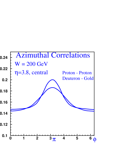
Figure 9: The azimuthal angle correlations of produced jets at forward direction with rapidity $\eta=3.8$. The value of the trigger momentum is taken $1.5\,GeV$ while the hadrons produced in the backward direction were integrated over transverse momenta from $0.2\,GeV$ to $1.5\,GeV$.

A most interesting opportunity to investigate the CGC dynamics in the quantum domain is to study reactions Les in which the trigger hadron with transverse momentum $p_{1}$ is generated in the forward direction ( say, $y_{1}=3.8$) while the recoiling particle(s) produced at the azimuthal angle $\phi$ is detected in the central rapidity region ($y_{2}=0$, see Fig. 10). The interest in this kinematics stems from the fact that a large rapidity interval $\Delta y=y_{1}-y_{2}$ between the detected particles enhances the effects of quantum evolution, since the probability of gluon emission is proportional to $\alpha_{s}\ \Delta y$. In fact, the study of gluon jets separated in rapidity has been proposed by Mueller and Navelet MuellerN as a way to investigate the properties of BFKL evolution. In the case of nuclear target, the quantum evolution enhances the influence of the saturation and extends it to larger transverse momenta.

The double inclusive cross section for such kinematics can be written in the form:

$$\frac{1}{\sigma}\,\frac{d\sigma}{dy_{1}\,d\,y_{2}\,\,d^{2}p_{1,t}\,d^{2}p_{t,2}}\,\,=\,\,\left(\frac{4N_{c}\,\alpha_{S}}{N^{2}-1}\right)^{2}\,\frac{1}{p^{2}_{1,t}}\,\frac{1}{p^{2}_{2,t}}\times$$ (14)

$$\int\,\,d^{2}\,k_{t}\,,d^{2}\,k^{\prime}_{t}\varphi_{projectile}\left(k^{2}_{t},Y-y_{1}\right)\,\,\varphi^{BFKL}\left(y_{1}-y_{2},k_{t},k^{\prime}_{t};\phi\right)\,\,\varphi_{target}\left(k^{\prime}_{t},y_{2}\right)$$

where $\varphi^{BFKL}$ is the BFKL scattering amplitude for two gluons. This amplitude takes into account the emission of gluons with rapidities between $y_{1}$ and $y_{2}$ (see Fig. 10). This amplitude can be written as series BFKL

$$\varphi^{BFKL}\left(y_{1}-y_{2},k_{t},k^{\prime}_{t};\phi\right)\,\,=\sum^{\infty}_{n=0}\,\,Cos(n\,\phi)\,\,\varphi^{BFKL}_{n}\left(y_{2}-y_{1},k_{t},k^{\prime}_{t}\right)$$ (15)

where $\phi$ is the azimuthal angle and $\varphi^{BFKL}_{n}$ are the eigenfunctions of the BFKL equation, which at high energies behave as

$$\varphi^{BFKL}_{n}\left(y_{2}-y_{1},k_{t},k^{\prime}_{t}\right)\,\,\,\rightarrow\,\,\,e^{\omega_{n}\,\,(y_{2}-y_{1})}$$ (16)

where

$$\omega_{n}\,\,\,=\,\,\,\frac{2\,\alpha_{S}N_{c}}{\pi}\,\left(\,\psi(1)\,\,-\,\,\psi(\frac{1}{2}+n)\,\right)$$ (17)

However, in Eq. (15) only the first term has a positive intercept ($\omega_{0}>0$) while all other terms fall off as a function of energy. Indeed, Eq. (17) gives

$$\omega_{0}\,\,=\,\,\frac{4\,\ln 2\,\alpha_{S}N_{c}}{\pi}\,\,\,\,\,\,;\,\,\,\,\,\omega_{1}\,\,=\,\,-\,\frac{1.22\,\alpha_{S}N_{c}}{\pi}\,\,\,\,\,\,;\,\,\,\,\,\omega_{2}\,\,=\,\,-\,\,\frac{2.56\,\alpha_{S}N_{c}}{\pi}$$

We thus replace $\varphi^{BFKL}$ by sum of two first terms with $n=0$ and $n=1$, since other terms are supressed at large value of $|y_{1}-y_{2}|.$

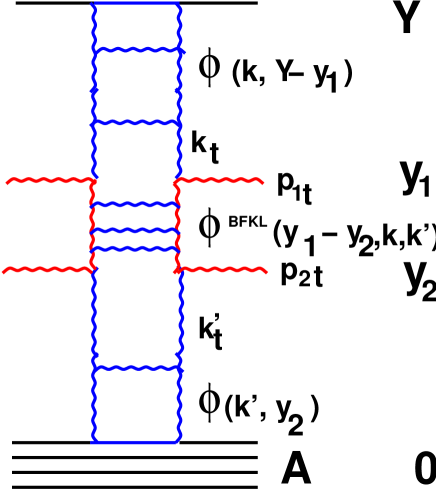
Figure 10: The BFKL emission in the double inclusive cross section.

Fig. 11 shows the normalized azimuthal distribution of the jets when the recoiling jet has $\eta_{2}=0$ and $0.2\,GeV\,\,<\,p_{2}\,<1.5\,GeV$ while the trigger jet has $\eta_{1}=3.8$ and $p_{1}=1.5\,GeV$ assuming that both of the jets are produced from one parton shower (see Fig. 3-a and Fig. 10). One can see that in both cases (for proton - proton and deuteron-gold collisions ) we expect sufficiently strong correlations. For deuteron-gold collision the width of the distribution in the azimuthal angle $\phi$ is only 30% larger than for the proton -proton scattering.

This result is not final though, since the main difference between the two cases is in the independent production from two parton showers ( see Fig. 4 ). In the CGC phase we have a saturation of the parton densities which is expressed in our assumption for the functions $\varphi$’s (see Eq. (7)). In this region the diagrams for independent two jet production (see Fig. 4 ) are much more important than the production of two jets from the single parton shower. Indeed, diagrams of Fig. 3-a and Fig. 10 lead to the cross section of the order of 1 while the independent production given by Fig. 4 leads to the cross section of the order of $(1/\alpha_{S}(Q_{s}))^{2}$. In reality, Fig. 11-b shows that the azimuthal correlation in deuteron - gold collision leads to a maximum around $\phi=\pi$ which the height of only 17%. For proton -proton we still expect a sizable effect of around 57%. One can see therefore that the quantum evolution effects in the CGC indeed induce a large difference between the back-to-back correlations expected in $pp$ and $dA$ collisions.

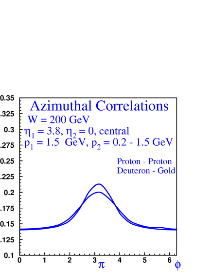
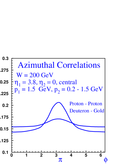
Fig. 11-a	Fig. 11-b

Figure 11: Fig. 11-a: The azimuthal angle correlations of produced jets in one parton shower at forward direction with rapidity $\eta_{2}=0$ and with $1.5\,GeV\,>\,p_{2}\,>\,0.4\,GeV$ when the trigger jet is at $\eta_{1}=3.8$ and with transverse momentum $p_{1}=1.5\,GeV$. Fig. 11-b: The azimuthal angle correlations of produced jets at forward direction with rapidity $\eta_{2}=0$ and with $1.5\,GeV\,>\,p_{2}\,>\,0.4\,GeV$ when the trigger jet is at $\eta_{1}=3.8$ and with transverse momentum $p_{1}=1.5\,GeV$. Both, production from one parton shower and from two parton showers are taken into account.

Let us now discuss the main uncertainties involved in our calculations. Our estimates of the independent production in comparison with the production in one parton shower have large errors because they involve the normalization of the inclusive cross section. The relative contribution of the diagram of Fig. 4 to the diagram of Fig. 3-a (we define $Z$ as a numerical factor which should stand in front of the diagram of Fig. 4 which is defined as the square of expression given by Eq. (4).) can be expressed through the normalization constant that we have introduced earlier in describing the multiplicity in d A collisions KLNDA . Denoting this constant by $C$ we have for the normalization of the relative contribution ($Z$) the following expression

$$Z\,\,=\,\,\frac{(N^{2}_{c}-1)\cdot C\cdot 4\pi}{9\,\alpha_{S}(Q_{s})\,n_{jet}}$$ (18)

where $n_{jet}$ is the hadron multiplicity of jet with transverse momentum $Q_{s}$. The uncertainty in calculation of $n_{jet}$ is large and in our numerical estimates we take $n_{jet}=1.5$. For proton -proton collisions we introduce an additional normalization factor. We need it to describe the relation beetwen the parton density and the saturation momentum for this case since we cannot trust the geometrical estimates of the area of interaction in this case, as discussed in KLNDA .

It is important to note that the uncorrelated production can be subtracted from the data experimentally since the inclusive cross section has been measured. Therefore, the correlation can be attributed to the diagrams of Fig. 10. In Fig. 12-a and Fig. 12-b we illustrate the azimuthal angle distribution for two different kinematic regions.

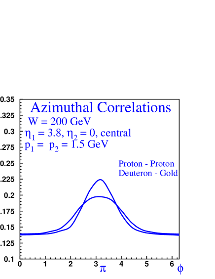
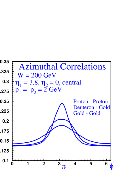
Fig. 12-a	Fig. 12-b

Figure 12: Fig. 12-a: The azimuthal angle correlations of produced jets at forward direction with rapidity $\eta_{2}=0$ and with $\,p_{2}\,\,=\,\,1.5\,GeV$ when the trigger jet is at $\eta_{1}=3.8$ and with transverse momentum $p_{1}=1.5\,GeV$. Only production from one parton shower is taken into account (see Fig. 10). Fig. 12-b: The azimuthal angle correlations of produced jets at forward direction with rapidity $\eta_{2}=0$ and with $\,p_{2}\,\,=\,\,2\,GeV$ when the trigger jet is at $\eta_{1}=3.8$ and with transverse momentum $p_{1}=2\,GeV$. Only production from one parton shower is taken into account (see Fig. 10).

These figures (Fig. 12-a and Fig. 12-b ) should be compared with Fig. 13, which gives the azimuthal correlations when both triggers have the same rapidity ($\eta_{1}=\eta_{2}=3.8$) and originate from the same parton shower.

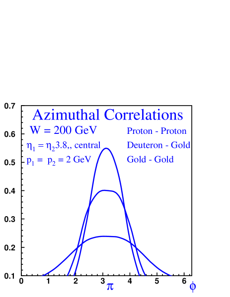
Figure 13: The azimuthal angle correlations of produced jets at forward direction with rapidity $\eta_{2}=0$ and with $\,p_{1}\,\,=\,p_{2}\,\,=\,\,2\,GeV$ when the trigger jet is at $\eta_{1}=\eta_{2}\,=\,3.8$. Only production from one parton shower is taken into account (see Fig. 10).

In fact one can substract the independent production of two hadrons just by measuring the inclusive cross section. The remaining emission in one parton shower then depends both on the saturation momenta for colliding hadron and/or nuclei and on the BFKL emission in the rapidity interval $\eta_{1}-\eta_{2}$. The prediction for this process is theoretically reliable and could provide the information on the values of the saturation momenta.

To summarize, we have found that hadron azimuthal correlations provide a stringent tests of the parton saturation in the Color Glass Condensate. When both hadrons are detected at central rapidity, our results show that $pp$ and $dA$ correlations are quite similar, with some broadening in the latter case, whereas the correlations in $AA$ are suppressed, mainly due to the large independent production background. A most interesting possibility is provided by the kinematics in which one of the hadrons is detected at forward rapidity and another at central rapidity. In this case the effects of quantum evolution in the CGC on the correlation function are strong, and enhance the influence of the saturation boundary. This leads to a significant difference between $pp$ and $dA$ correlation functions.

References

-
(1)
R Debbe [BRAHMS Collaboration], Talk at the Fall 2003 DNP
Meeting, Tucson, Arizona, October 2003, and at Quark Matter 2004 Conference, Oakland, California, January 2004;
I. Arsene et al [BRAHMS Collaboration], arXiv:nucl-ex/0403005. - (2) M. Liu [PHENIX Collaboration], Talk at Quark Matter 2004 Conference, Oakland, California, January 2004; arXiv:nucl-ex/0403047.
- (3) P. Steinberg [PHOBOS Collaboration], Quark Matter 2004 Conference, Oakland, California, January 2004.
- (4) L. Barnby [STAR Collaboration], Quark Matter 2004 Conference, Oakland, California, January 2004.
- (5) D. Kharzeev, E. Levin and L. McLerran, Phys. Lett. B561 (2003) 93 [arXiv:hep-ph/0210332].
- (6) D. Kharzeev, Y. Kovchegov and K. Tuchin, Phys. Rev. D68 (2003) 094013.
- (7) J. L. Albacete, N. Armesto, A. Kovner, C. Salgado and U. Wiedemann, hep-ph/0307179
- (8) R. Baier, A. Kovner and U. Wiedemann, Phys.Rev.D68:054009,2003
- (9) L. V. Gribov, E. M. Levin and M. G. Ryskin, Phys. Rep. 100 (1983) 1.
-
(10)
A.H. Mueller and J. Qiu, Nucl.Phys. B 268 (1986) 427;
J.-P. Blaizot and A.H. Mueller, Nucl. Phys. B 289 (1987) 847. - (11) L. McLerran and R. Venugopalan, Phys. Rev. D 49 (1994) 2233; 3352; D 50 (1994) 2225.
- (12) E. Iancu, A. Leonidov and L. McLerran, Nucl.Phys.A692:583-645,2001; E. Iancu, E. Ferreiro, A. Leonidov and L. McLerran, Nucl.Phys.A703:489-538,2002.
- (13) E. Laenen and E. Levin, Ann. Rev. Nuc. Part. Sci. 44 (1994) 199; Yu. V. Kovchegov and D. Rischke, Phys. Rev. C56 (1997) 1084; M. Gyulassy and L. McLerran, Phys. Rev. C56 (1997) 2219; Yu. V. Kovchegov and A. H. Mueller, Nucl. Phys. B529 (1998) 451 M. A. Braun, Eur. Phys. J. C16 (2000) 337, hep-ph/0010041, hep-ph/0101070; Yu. V. Kovchegov, Phys. Rev. D64 (2000) 114016; Yu. V. Kovchegov and K. Tuchin, Phys. Rev. D65 (2002) 074026 hep-ph/0111362.
- (14) D. Kharzeev and M. Nardi, Phys. Lett. B507 (2001) 121.
- (15) D. Kharzeev and E. Levin, Phys. Lett. B523 (2001) 79; nucl-th/0108006.
- (16) D. Kharzeev, E. Levin and M. Nardi, “The onset of classical QCD dynamics in relativistic heavy ion collisions,” hep-ph/0111315.
- (17) D. Kharzeev, E. Levin and M. Nardi, Nucl. Phys. A 730, 448 (2004) and Erratum in arXiv:hep-ph/0212316.
- (18) J. Adams, Phys. Rev. Lett. 91 (2003) 072304; C. Adler, Phys. Rev. Lett. 90 (2003) 082302
- (19) Y. V. Kovchegov and K. L. Tuchin, Nucl. Phys. A 708, 413 (2002) [arXiv:hep-ph/0203213]; Nucl. Phys. A 717, 249 (2003) [arXiv:nucl-th/0207037].
- (20) V. A. Abramovsky, V. N. Gribov and O. V. Kancheli, Yad. Fiz. 18 (1973) 595 [Sov. J. Nucl. Phys. 18 (1974) 308].
- (21) Yu.V. Kovchegov, Phys. Rev. D 54 (1996) 5463; J. Jalilian-Marian, A. Kovner, L. McLerran, H. Weigert, Phys.Rev. D55 (1997) 5414; E. Iancu and L. McLerran, Phys.Lett. B510 (2001) 145; A. Krasnitz and R. Venugopalan, Phys. Rev. Lett.84 (2000) 4309; E. Levin and K. Tuchin, Nucl. Phys. B573 (2000) 833; A693 (2001) 787; A691 (2001) 779; A.H. Mueller,“Parton saturation: An overview,” hep-ph/0111244; E. Iancu, A. Leonidov and L. D. McLerran, Nucl. Phys. A692 (2001) 583, hep-ph/0011241; E. Iancu, K. Itakura and L. McLerran, Nucl. Phys. A708 (2002) 327, hep-ph/0203137.
- (22) Yu. V. Kovchegov and A. H. Mueller, Nucl. Phys. B529 (1998) 451
- (23) A. Szczurek, “From unintegrated gluon distributions to particle production in hadronic collisions at high energies,” arXiv:hep-ph/0309146; Acta Phys. Polon. B 34 (2003) 3191 [arXiv:hep-ph/0304129].
- (24) STAR collaboration: J. Adam et al., Phys. Rev. Lett. 91 (2003) 072304.
- (25) K. Golec-Biernat and M. Wüsthof, Phys. Rev. D59 (1999) 014017; Phys. Rev. D60 (1999) 114023; A. Stasto, K. Golec-Biernat and J. Kwiecinski, Phys. Rev. Lett. 86 (2001) 596.
- (26) B. A. Kniehl, G. Kramer and B. Potter, Nucl. Phys. B582 (2000) 514 [arXiv:hep-ph/0010289].
- (27) A. Ogawa (for the STAR Collaboration), AIP Conf. Proc. 675, 407 (2003).
- (28) A.H. Mueller and H. Navelet, Nucl. Phys. B 282 (1987) 727.
-
(29)
E.A. Kuraev, L.N. Lipatov and V.S. Fadin, Sov. Phys. JETP 45,
199 (1977);
Ya.Ya. Balitskii and L.V. Lipatov, Sov. J. Nucl. Phys. 28, 822 (1978);
L.N. Lipatov, Sov. Phys. JETP 63, 904 (1986).