11institutetext: Universit a di Genova, Sezione INFN di Genova, via Dodecaneso 33, 16142 Genova (Italy) 22institutetext: Institut für Kernphysik, Universität Mainz, Staudingerweg 45, 55099 Mainz (Germany)
Generalized sum rules of the nucleon in the constituent quark model
M. Gorchtein
11D. Drechsel
22M. Giannini
11E. Santopinto
11
The sum rules serve a
powerful tool to study the nucleon structure by providing a bridge
between the statical properties of the nucleon (such as electrical charge,
and magnetic moment) and the dynamical properties (e.g. the transition
amplitudes to excited states) in a wide range of energy and momentum
transfer . We study the generalized sum rules of the nucleon in the
framework of the constituent quark model. We use two different CQM, the one
with the hypercentral potential hccqm1 , hccqm2 , hccqm3 ,
and with the harmonic oscillator potential KI ,
both with only few parameters fixed to the baryonic spectrum.
We confront our results to the model independent sum rules and to the
predictions of the phenomenological MAID MAID model and find that
in all the cases
considered, in the intermediate range (0.2-1.5 GeV2), both CQM
models provide a good description of the sum rules on the neutron.
pacs:
12.39.JhNonrelativistic quark model and 14.20.GkBaryon resonances and helicity amplitudes
1 Introduction
In the recent years, precise measurements of single and double polarization
observables for the photo- and electorabsorption have become possible.
The inclusive cross section for the process
can be written in terms of the four partial cross
sections,
(1)
with ,
,
the virtual photon flux factor , and the photon polarization
, where
denote the initial (final) electron energy, the
energy transfer to the target, the electron c.m. scattering angle,
and the four momentum transfer. The virtual photon
spectrum normalization factor is chosen to be ,
refers to the electron helicity,
while and are the components of the target polarization.
For a general and complete consideration of the nucleon sum rules we readress
the reader to the review reviewdr .
2 Constituent quark model
We study the generalized sum rules for the nucleon within a
hyper central constituent quark model (HCCQM) previously reported in
hccqm1 , hccqm2 , hccqm3 . The model based on the lattice
QCD inspired potential of the form
and allows
for a consistent description of the baryonic spectrum with a minimal number of
parameters. Furthermore, to display the
model dependence of a CQM calculation, we list also the results within the
CQM with a harmonic oscillator (HO) potential. Within this
model, we for the first time report a calculation of the longitudinal
amplitudes and their contribution to the sum rules, details of which will be
reported in an upcoming article.
The electromagnetic transition helicity amplitudes are defined as
(2)
where , stands for the spin projection of the
initial (nucleon) and final (resonance) hadronic state, and the definition was
used,
.
We will present the results for the sum rules within the
approximation where one has for the contribution of a single resonance to
the partial cross sections
(3)
with , ,
and the resonance mass.
3 Sumrules for the forward polarizabilities of the proton
We start with the Baldin sum rule which relates the sum of the electromagnetic
polarizabilities to the integral over the total photoabsorption cross section,
(4)
where is the pion production threshold.
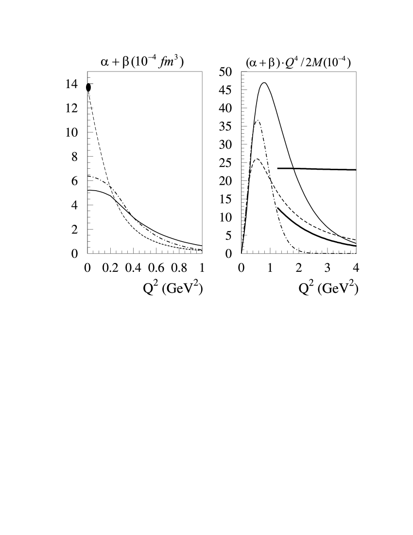
Figure 1: Results for the sum of the proton polarizabilities
calculated in HCCQM (solid line), HO model (dashed-dotted line)
in comparison with MAID (dashed line). The solid circle corresponds to the
Baldin sum rule value at MAMI .
As it can be seen from Fig. 1, both constituent quark models
fall short at by a factor of 3, which is a consequence of lacking
the large contribution of pion production.
However, starting from GeV2 all three models give similar results.
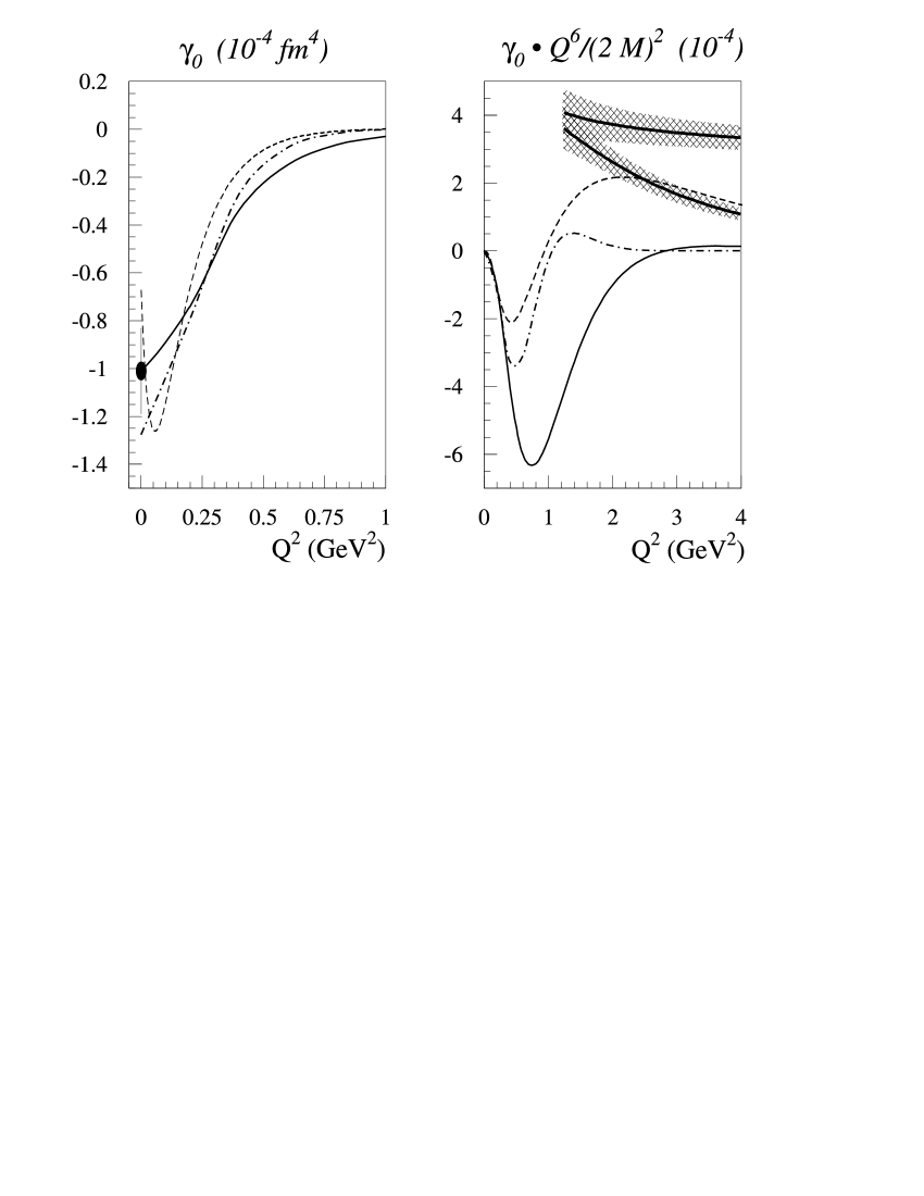
We next turn to the sum rules with the helicity flip cross section
. In Fig. 2, we show the results for the forward
spin polarizability,
(5)
In the case of , the small value phenomenologically comes about
due to a strong
cancellation of a large negative contribution of the
resonance, and a large positive contribution of near threshold pion production.
Though the latter is not present in neither of the two presented quark model
calculations, both do surprisingly well for this sum rule, as can be seen in
Fig. 2, since almost all the transition helicity amplitudes in
a CQM lack strenght, as compared to the phenomenological analysis. Therefore,
the fact that the quark model results are consistent with the results of MAID
in the shown range of should be seen rather as a coincidence. It is
interesting to note that, due to the characteristical for the HO potential
gaussian form factors, the HO model closely reproduces the slope of the MAID
curve.
Figure 2: Results for on proton. Notation as in Fig.
1. The data point at is from MAMI .
4 Generalized GDH sum rule
The GDH sum rule relates the anomalous magnetic moment of the nucleon
to the integral over its excitation spectrum,
(6)
thus providing a test of a quark model, since both left and right hand sides
of this sum rule can be calculated. One of the possible generalizations of
this integral to the case of finite is
(7)
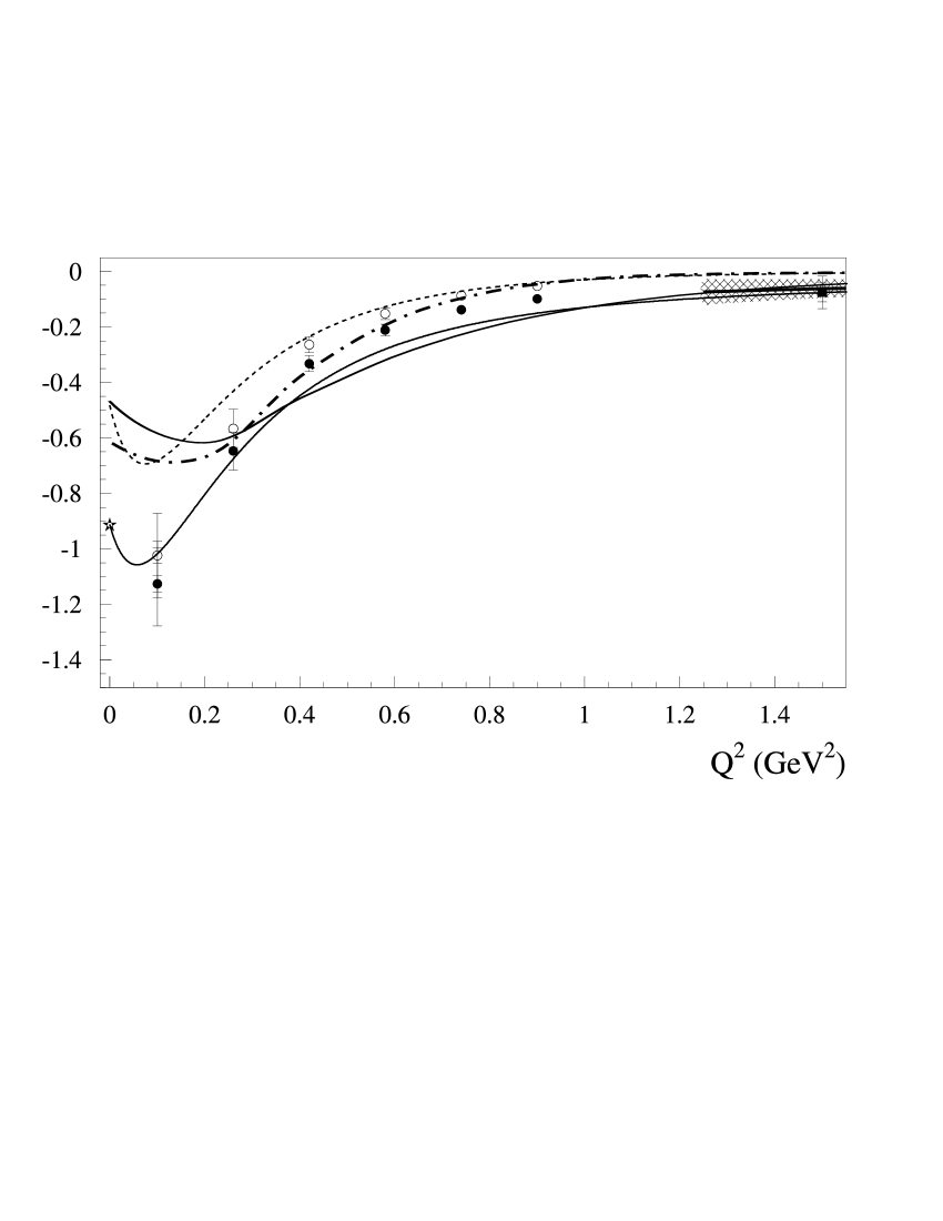
In Fig. 3, we show the results for the GDH integral on
the neutron. As one can see, the sum rule at the real photon point
is not obeyed in either quark model.
Figure 3: Results for the generalized GDH integral . Notation as in
Fig. 1.
The thin solid line corresponds to the experimental fit,
as described in text. The solid line starting from 1.25 GeV2 corresponds
to the evaluation of the GDH integral using the data on the DIS structure
functions (for the details, see reviewdr ). The solid star represents
the sum rule value at . The data points are from
HERMES (solid squares) and
IAnJLAB (solid (full result) and open (resonant part with
GeV) circles).
Starting from GeV2, the
HCCQM practically follows the experimental fit, which assumes the following
form (for details, see reviewdr ):
(8)
with and the resonance part as calculated with MAID.
Due to the characteristical
HO gaussian form factors having a more steep dependence, the HO model
is able to reproduce the data up to 1 GeV, but falls short beyond this
region.
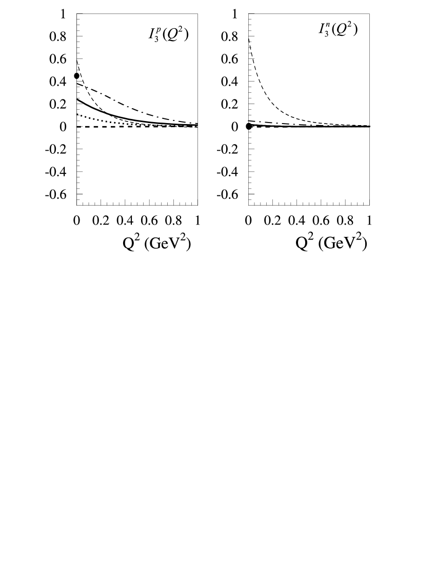
5 Sum rule for the integral
The only sum rule containing a prediction for the electric charge
of the nucleon is
(12)
In Fig. 4, we show the results for the integral on the
neutron. While the MAID prediction is in complete disagreement with the
sum rule value, one can see that the HCCQM result differs only slightly from
zero, as required by the sum rule, and HO model gives a small
positive value. Apart from the different potential of the two CQM models, the
presented HO calculation does not take account of the hyperfine
mixing of the wave functions which may be responsible for the cancellation
within this integral.
Figure 4: Results for the integral for the neutron. Notation as
in Fig. 1. Solid cicrcle corresponds to the sum rule value.
References
(1) M. Ferraris, M.M. Giannini, M. Pizzo, E. Santopinto, L. Tiator
PL B 364 (1995) 231-238.
(2) M. Aiello, M. Ferraris, M.M. Giannini, M. Pizzo, E. Santopinto
PL B 387 (1996) 215-221.
(3) M. Aiello, M.M. Giannini, E. Santopinto,
J. Phys. G: Nucl. Part. Phys. 24 (1998) 753-762.
(4) N. Isgur and G. Karl, Phys. Rev. D 18 4187.
(5) D. Drechsel, O. Hanstein, S. Kamalov, L. Tiator
Nucl. Phys. A 645 (1999) 145.
(6) D. Drechsel, B. Pasquini, M. Vanderhaeghen
Phys. Rept. 378 (2003) 99-205, and references therein.
(7) J. Ahrens et al. (GDH and A2 Collaboration),
Phys. Rev. Lett. 84 (2000) 5950.
(8) A. Airapetian et al. (HERMES Collaboration),
Eur. Phys. J. C26 (2003) 527.
(9) M. Amarian et al. (JLab E94010 collaboration),
Phys. Rev. Lett. 89 (2002) 242301.