Effects of perturbative exchanges in a QCD–string model

Abstract

The QCD-string model for baryons derived by Simonov and used for the calculation of baryon magnetic moments in Ref. Simonov et al. (2002) is extended to include also perturbative gluon and meson exchanges. The mass spectrum of the baryon multiplet is studied. For the meson interaction either the pseudoscalar or pseudovector coupling is used. Predictions are compared with the experimental data. Besides these exchanges the influence of excited quark orbitals on the baryon ground state are considered by performing a multichannel calculation. The nucleon-$\Delta$ splitting increases due to the mixing of higher quark states while the baryon magnetic momenta decrease. The multichannel calculation with perturbative exchanges is shown to yield reasonable magnetic moments while the mass spectrum is close to experiment.

1 Introduction

As QCD is generally accepted as the theory of strong interactions, $\bar{q}q$ and $3q$ dynamics should be derived from QCD in a fully relativistically covariant way. This is a formidable task due to the large gluon-quark coupling constant in the low energy regime and the non-Abelian character of QCD. In recent years the formalism of field correlators was set up to deal with the two main characteristics of quark-systems: confinement and chiral symmetry breaking. Using this field correlator method (FCM) a nonlinear equation has been derived for a light quark in the field of a heavy antiquark Simonov (1997, 1998). In the derivation use has been made of the large $N_{c}$ limit and the calculation has been restricted to include only the Gaussian (bilocal) field correlator, an approximation which has been shown to be correct within a few percent by lattice simulations as was discussed in Ref. Shevchenko and Simonov (2000).

The developed method is quite general and can be extended to treat the light quark systems $\bar{q}q$ and $3q$ as was shown in Refs. Simonov et al. (2002); Simonov (1999). Using this formalism the baryon magnetic moments and corrections on these from virtual mesonic excitations have been calculated. Reasonable agreement with experiment has been obtained without the need of introduction of constituent quark masses Simonov et al. (2002). The outcome of the method is partially summarized in the next section.

In the present paper we extend the model in the following way. Using the same formalism as in Ref. Simonov et al. (2002) to obtain the baryon wave functions, the baryon mass spectrum of the lowest octet and decuplet representation of the $SU(3)$-flavor group is obtained. In section 3 perturbative corrections to this spectrum due to one gluon (OGE) and pseudoscalar meson exchanges are calculated. For the coupling of the pseudoscalar mesons to the quark both pseudoscalar and pseudovector couplings are exploited. Following Refs. Isgur and Karl (1978, 1979); Capstick and Isgur (1986) we consider the influence of excited states to the ground state. This is done by forming excited baryon states out of the orbital and radial excitations of the single-quark wave functions and using these as a basis to diagonalize the Hamiltonian. The results from the multichannel calculation are shown in section 4. The consequences of the diagonalization of the Hamiltonian to the magnetic moments are calculated in section 5. The paper ends with some discussions in section 6.

2 Formalism

As was explained in Refs. Simonov et al. (2002); Simonov (1999) the field correlator method can be used to obtain an effective quark Lagrangian $L_{eff}$ from the QCD-partition function. Integrating out the gluon fields by using the generalized Fock-Schwinger gauge with contour $C$ Shevchenko and Simonov (1998); Ivanov and Korchemsky (1985); Ivanov et al. (1986) the QCD action can be rewritten as

$$Z=\int D\kappa(C)D\Psi D\Psi^{\dagger}exp\leavevmode\nobreak\ ({L_{0}+L_{eff}}),$$ (1)

where $L_{0}$ is the free quark field Lagrangian and the effective Lagrangian in lowest order in quark fields has the form of a nonlocal four-fermion interaction. Moreover, since $Z$ is gauge invariant we have introduced an additional integration over a set of contours $C(k)$ with weight $D\kappa(C)$ in the partition function. In the field correlator method the Gaussian approximation is usually made, which is has been discussed extensively in Refs. Shevchenko and Simonov (2000); Simonov (2000). Choosing the generalized Fock-Schwinger gauge Shevchenko and Simonov (1998); Ivanov and Korchemsky (1985); Ivanov et al. (1986) with contours going through a given point ${\bf r_{0}}$ an effective action is determined. In this way a Hamiltonian equation has been derived for the baryon, depending on the parameter ${\bf r_{0}}$,

$$(H_{1}+H_{2}+H_{3}-E)\Psi(\mbox{\boldmath${\rm r}$}_{1},\mbox{\boldmath${\rm r}$}_{2},\mbox{\boldmath${\rm r}$}_{3})=0,$$ (2)

with

$$H_{i}=m_{i}\beta^{(i)}+\mbox{\boldmath${\rm p}$}_{i}\mbox{\boldmath${\rm\alpha}$}^{(i)}+\beta^{(i)}M_{i}(\mbox{\boldmath${\rm r}$}_{i}-\mbox{\boldmath${\rm r}$}_{0}).$$ (3)

The quark mass operator $M_{i}$ produces both linear confinement and chiral symmetry breaking as was shown in Refs. Simonov and Tjon (2000a); Simonov (1997, 1998). It is a nonlinear and nonlocal operator acting in the coordinate space of the $i$-th quark. When only the dominant part of $M_{i}$ leading to confinement is kept, the kernel can be characterized as

$$M(x,y)\approx\leavevmode\nobreak\ \frac{1}{2T_{g}\sqrt{\pi}}\sigma\left|\frac{\mbox{\boldmath${\rm x}$}+\mbox{\boldmath${\rm y}$}}{2}\right|\exp\left(-\frac{({\bf x}-{\bf y})^{2}}{4T_{g}^{2}}\right),$$ (4)

where $T_{g}$ is the gluon correlation length corresponding to the length scale of correlations in the fluctuations of the gluon background field. From lattice gauge simulations it has been found to be of the order of $\frac{1}{4}\leavevmode\nobreak\ fm$. Following Ref. Simonov and Tjon (2000a) we have adopted a value $T_{g}=0.24\leavevmode\nobreak\ fm$. For asymptotic large $|x|$ it has been shown that the kernel Eq. (4) leads for a fixed ${\bf r_{0}}$ to a linear confining interaction $\sigma|{\bf r_{i}}-{\bf r_{0}}|$ Simonov and Tjon (2000a, b). Moreover, it is of a Lorentz-scalar type. In this paper we will also allow for a constant term in the confining interaction, corresponding to the next leading order corrections to the area law. The weight $D\kappa(c)$ should be chosen as a stationary point of the effective action and that the contours generate a string of minimal length. As a consequence the parameter $\mbox{\boldmath${\rm r}$}_{0}$ can in principle be found as the minimum of the interaction between the three quarks, yielding for $\mbox{\boldmath${\rm r}$}_{0}$ the so-called Torricelli point. This would result in a single string Y-junction which is of a genuine three-body nature. However, for practical reasons, we take as a first approximation $\mbox{\boldmath${\rm r}$}_{0}$ as a constant parameter as was done in Ref. Simonov et al. (2002). Due to treating $\mbox{\boldmath${\rm r}$}_{0}$ as a constant instead of adopting the Torricelli point $\mbox{\boldmath${\rm r}$}_{T}$, the distance $\sum_{i=1}^{3}\left|\mbox{\boldmath${\rm r}$}_{i}-\mbox{\boldmath${\rm r}$}_{0}\right|$ is about $\sim 2.5$ times bigger than the minimal distance $\sum_{i=1}^{3}\left|\mbox{\boldmath${\rm r}$}_{i}-\mbox{\boldmath${\rm r}$}_{T}\right|$. This means that the string tension $\sigma$ has to be chosen $\sim 2.5$ times smaller to yield about the same energy. Recent lattice simulations on static quarks obtain a value of about $\sigma=0.15\leavevmode\nobreak\ \text{GeV}^{2}$ for the three-quark Y-shaped interaction which is close to the value for quark-antiquark interactions Takahashi et al. (2001). This result suggests that string tensions as low as $\sigma=0.06\leavevmode\nobreak\ \text{GeV}^{2}$ can be used in our calculations.

The solution of Eq. (2) is now of a factorizable form which enables us to represent the baryon wave function as the product of three single particle solutions,

$$\Psi_{JM}=\Gamma^{\alpha\beta\gamma}_{JM}(f_{1}f_{2}f_{3})e_{abc}\psi^{f_{1}}_{a\alpha}(\mbox{\boldmath${\rm r}$}_{1}-\mbox{\boldmath${\rm r}$}_{0})\psi^{f_{2}}_{b\beta}(\mbox{\boldmath${\rm r}$}_{2}-\mbox{\boldmath${\rm r}$}_{0})\psi^{f_{3}}_{c\gamma}(\mbox{\boldmath${\rm r}$}_{3}-\mbox{\boldmath${\rm r}$}_{0}),$$ (5)

where $a,\leavevmode\nobreak\ b,\leavevmode\nobreak\ c$ and $f_{i}$ are the color and flavor indices respectively. The orbital and radial excitations are indicated by $\alpha$, $\beta$ and $\gamma$. Because of the Pauli principle the baryon wave function has to be a total antisymmetric function of the three quark functions. As the baryon is a color white object (antisymmetric in color), the wave function Eq. (5) has to be total symmetric in flavor, orbital and radial excitations of the single particle wave functions $\psi^{f_{i}}_{a\alpha}$. The functions $e_{abc}$ and $\Gamma^{\alpha\beta\gamma}_{JM}$ respectively take care of this (anti)-symmetrization. Explicit formulas for the lowest baryons are given in Appendix A.

Each single particle solution satisfies a nonlinear Dirac-like Hamiltonian equation,

$$H_{i}\psi^{f_{i}}_{a_{i}\alpha_{i}}=\varepsilon_{n_{i}}^{(i)}\psi^{f_{i}}_{a_{i}\alpha_{i}},\qquad E=\sum_{i=1}^{3}\varepsilon_{n_{i}}^{(i)}.$$ (6)

where $H_{i}$ is given by Eq. (3). It has to be solved self consistently, leading to confining solutions. Details can be found in Ref. Simonov and Tjon (2000a). In table 1 some values of $\varepsilon_{n}$ are shown. The solutions are listed as

$$n(j)^{{\rm sign}(\kappa){\rm sign}(\varepsilon_{n})},\qquad\kappa=\pm\left(j+\tfrac{1}{2}\right).$$ (7)

From these single-quark orbitals the baryon spectrum $M_{B}=E$ and the corresponding baryon wave funtions, Eq. (5), can immediately be constructed.

Using these baryon wave functions the magnetic moments $\mu_{z}$ have been determined in Ref. Simonov et al. (2002). Following Ref. Kloet and Tjon (1971) we have

$$\mu_{z}=\frac{e}{2M_{p}}G_{mag}(Q=0)=-\frac{i}{2}\left[\mbox{\boldmath${\rm\nabla}$}_{Q}\times\mbox{\boldmath${\rm M}$}\right]_{z}({Q=0}),$$ (8)

where $e$, $M_{p}$ and $G_{mag}$ are the charge, mass and Sachs magnetic moment of the proton. The electromagnetic current matrix element $M_{\mu}$ is given by

$$M_{\mu}=\left<\Psi\left|J_{\mu}(Q)\right|\Psi\right>.$$ (9)

For the operator $J_{\mu}$ the single-quark current operator is taken as the first approximation. Higher order contributions come from two-body currents like one-pion-exchange currents and mesonic one-loop corrections which give rise to the anomalous magnetic moment of the quark. Reasonable values were obtained for the magnetic moments of the baryon octet and decuplet in the case of a string tension of $\sigma=0.1\leavevmode\nobreak\ \text{GeV}^{2}$ without the need of introduction of constituent quark masses Simonov et al. (2002). In the present paper we extend this analysis to also include the one-gluon-exchange and study the effects of the use of different forms for the interaction in the one-pion-exchange.

3 Exchange potentials

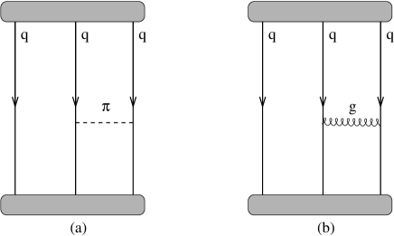
5mm normal

Figure 1: A schematic view of the exchange of a pion (a) and a gluon (b) between two quarks in a baryon. The blobs at the beginning and the end of the diagram represent bound states of the quarks.

Until now the picture of quarks moving in the confining sea of gluons is used. This leads to confinement and chiral symmetry breaking, but it lacks spin-dependent interactions. Typical spin-dependent structures in the baryon spectrum as the splitting between the nucleon and the $\Delta$ are therefore not present in such a simplified model. To remove this deficiency a perturbative one-gluon-exchange interaction is now introduced. The Coulomb part is expected to lower the baryon masses and the color magnetic part is expected to give rise to a splitting between the $J=1/2$ and $J=3/2$ states. Beside this one-gluon interaction we also introduce perturbative pseudoscalar meson-exchanges which can be considered as an effective interaction representing the exchange of correlated quark anti-quark pairs. The interactions are schematically shown in Figure 1.

The Hamiltonian equation, Eq. (2), is equivalent to a Bethe-Salpeter equation with an instantaneous interaction. Of all possible three particle wave functions of the type (5) it couples only to $(+++)$ and $(---)$, where $\pm$ indicates the sign of $\epsilon_{n}$ as in Eq. (7). All other wave functions decouple. Within such an equal time approximation we now consider the effects of the perturbative exchanges. Following Refs. Loring et al. (2001); Metsch (1997); Metsch and Loring (2002) where the instantaneous three particle Bethe-Salpeter equation is considered, we assume that the perturbative gluon- and meson-exchanges only take place between these purely positive and negative energy components. As discussed in Ref. Loring et al. (2001) we write for the interaction potential in the Hamiltonian,

$$H_{\rm int}^{(23)}\Psi(P,\mbox{\boldmath${\rm p}$}^{\prime}_{\rho},\mbox{\boldmath${\rm p}$}^{\prime}_{\lambda})=\left(\Lambda^{+}(\mbox{\boldmath${\rm p}$}_{1})\Lambda^{+}(\mbox{\boldmath${\rm p}$}_{2})\Lambda^{+}(\mbox{\boldmath${\rm p}$}_{3})+\Lambda^{-}(\mbox{\boldmath${\rm p}$}_{1})\Lambda^{-}(\mbox{\boldmath${\rm p}$}_{2})\Lambda^{-}(\mbox{\boldmath${\rm p}$}_{3})\right)\\ \times\int\frac{d^{3}p^{\prime}_{\rho}}{(2\pi)^{3}}\frac{d^{3}p^{\prime}_{\lambda}}{(2\pi)^{3}}\gamma^{0}_{(2)}\gamma^{0}_{(3)}V_{\rm ex}^{(23)}(\mbox{\boldmath${\rm p}$}_{\rho},\mbox{\boldmath${\rm p}$}_{\lambda},\mbox{\boldmath${\rm p}$}^{\prime}_{\rho},\mbox{\boldmath${\rm p}$}^{\prime}_{\lambda})\Psi(P,\mbox{\boldmath${\rm p}$}^{\prime}_{\rho},\mbox{\boldmath${\rm p}$}^{\prime}_{\lambda}),$$ (10)

with the energy projection operators defined as

$$\Lambda^{\pm}(\mbox{\boldmath${\rm p}$})=\frac{\omega\pm H(\mbox{\boldmath${\rm p}$})}{2\omega},\qquad\omega=\left|\epsilon_{n}\right|.$$ (11)

The interactions between the other quark pairs, $H_{\rm int}^{(12)}$ and $H_{\rm int}^{(13)}$, can very similarly be written down and easily be included. The Hamiltonian equation Eq. (2) becomes

$$H\Psi(\mbox{\boldmath${\rm r}$}_{1},\mbox{\boldmath${\rm r}$}_{2},\mbox{\boldmath${\rm r}$}_{3}) =\left(H_{1}+H_{2}+H_{3}+H_{\rm int}^{(12)}+H_{\rm int}^{(13)}+H_{\rm int}^{(23)}\right)\Psi(\mbox{\boldmath${\rm r}$}_{1},\mbox{\boldmath${\rm r}$}_{2},\mbox{\boldmath${\rm r}$}_{3})$$

$$=\left(E+\Delta E\right)\Psi(\mbox{\boldmath${\rm r}$}_{1},\mbox{\boldmath${\rm r}$}_{2},\mbox{\boldmath${\rm r}$}_{3}).$$ (12)

The exchange interactions are treated perturbatively,

$$\Delta E=3\left\langle\Psi_{JM}\left|H_{\rm int}^{(23)}\right|\Psi_{JM}\right\rangle,$$ (13)

where $\Psi_{JM}$ represents the baryon wave function, Eq. (5). Because of symmetry considerations the interactions between the other quark pairs can simply be included by adding a factor of 3 shown in Eq. (13).

The exchange potential $V_{\rm ex}^{(23)}$ in Eq. (10) for the non-strange baryons can be split into two contributions, the one gluon exchange (OGE) and the one-pion-exchange (OPE). They are explicitly written as,

$$V_{oge}^{(23)}(\mbox{\boldmath${\rm k}$}) =-4\pi\frac{2}{3}\alpha_{s}\frac{\gamma_{\mu}(2)\gamma^{\mu}(3)}{\mbox{\boldmath${\rm k}$}^{2}},$$ (14a)

$$V_{ope}^{(23)}(\mbox{\boldmath${\rm k}$}) =4\pi g_{qq\pi}^{2}\mbox{\boldmath${\rm\tau}$}(2).\mbox{\boldmath${\rm\tau}$}(3)\gamma_{5}(2)\gamma_{5}(3)\frac{1}{\mbox{\boldmath${\rm k}$}^{2}+m_{\pi}^{2}}\left(\frac{\Lambda^{2}}{\mbox{\boldmath${\rm k}$}^{2}+\Lambda^{2}}\right)^{2},$$ (14b)

where a pseudoscalar (PS) coupling for the pion is assumed. The factor $2/3$ in the OGE originates from the color content of the baryons and the term $\mbox{\boldmath${\rm\tau}$}(2).\mbox{\boldmath${\rm\tau}$}(3)$ in the OPE takes care of the isospin. The exchange potentials can also be written in coordinate space by performing Fourier transformations

$$V_{oge}^{(23)}(\mbox{\boldmath${\rm r}$}_{2}-\mbox{\boldmath${\rm r}$}_{3}) =-\frac{2}{3}\alpha_{s}\frac{\gamma_{\mu}(2)\gamma^{\mu}(3)}{\left|\mbox{\boldmath${\rm r}$}_{2}-\mbox{\boldmath${\rm r}$}_{3}\right|},$$ (15a)

$$V_{ope}^{(23)}(\mbox{\boldmath${\rm r}$}_{2}-\mbox{\boldmath${\rm r}$}_{3}) =g_{qq\pi}^{2}\mbox{\boldmath${\rm\tau}$}(2).\mbox{\boldmath${\rm\tau}$}(3)\gamma_{5}(2)\gamma_{5}(3)\left(\frac{\Lambda^{2}}{\Lambda^{2}-m_{\pi}^{2}}\right)^{2}$$ (15b)

$$\quad\times\left(-\frac{e^{-m_{\pi}\left|\mbox{\boldmath${\rm r}$}_{2}-\mbox{\boldmath${\rm r}$}_{3}\right|}}{\left|\mbox{\boldmath${\rm r}$}_{2}-\mbox{\boldmath${\rm r}$}_{3}\right|}+\frac{e^{-\Lambda\left|\mbox{\boldmath${\rm r}$}_{2}-\mbox{\boldmath${\rm r}$}_{3}\right|}}{\left|\mbox{\boldmath${\rm r}$}_{2}-\mbox{\boldmath${\rm r}$}_{3}\right|}+\frac{\Lambda^{2}-m_{\pi}^{2}}{\Lambda}\frac{e^{-\Lambda\left|\mbox{\boldmath${\rm r}$}_{2}-\mbox{\boldmath${\rm r}$}_{3}\right|}}{2}\right),\qquad\text{(PS)}.$$

Details on the calculation of the perturbative calculation of the matrices Eq. (13) can be found in appendix B.

When a pseudovector (PV) pion-quark coupling is assumed some modifications have to be made. In Eq. (14b) the pseudovector coupling is obtained by the replacement

$$g_{\pi qq}\gamma_{5}\tau_{a}\rightarrow\frac{g_{\pi qq}}{2m_{eff}}\gamma_{5}\not\!k\tau^{a},$$ (16)

where $m_{eff}$ is a scaling mass of the order of the constituent quark mass, to be discussed later. By Fourier transformation the momenta in Eq. (16) turn into derivatives in coordinate space. In this way the matrices $\not\!k$ can be evaluated when they act upon the quark wave functions resulting in some derivatives on the radial wave function and a changed angular dependence. Details are given in Appendix B.

The model can easily be extended to include the strange baryons. Apart from pion exchanges we now also have to add kaon and eta exchanges. These exchanges can be included by changing the SU(2) isospin matrices $\mbox{\boldmath${\rm\tau}$}_{2}.\mbox{\boldmath${\rm\tau}$}_{3}$ in Eq. (14b) into SU(3) flavor matrices $\sum_{a=1}^{8}\lambda_{2}^{a}\lambda_{3}^{a}$ and substituting the correct coupling constants, meson and cutoff masses.

For the coupling of the gluon to the quark a running coupling constant is used which depends on the distance. Following Ref. Badalian and Kuzmenko (2002) the coupling is parameterized as

$$\alpha^{(2)}(q)=\alpha^{(1)}(q)\left(1-\frac{\beta_{1}}{\beta_{0}^{2}}\frac{\ln t_{B}}{t_{B}}\right),\qquad\alpha^{(1)}(q)=\frac{4\pi}{\beta_{0}t_{B}},$$ (17)

with

$$t_{B}=\ln\frac{q^{2}+m_{B}^{2}}{\Lambda_{V}^{2}},$$ (18)

and

$$\beta_{0}=11-\frac{2}{3}n_{f},\qquad\beta_{1}=102-\frac{38}{3}n_{f}.$$ (19)

As the calculation is performed in coordinate space, the coupling constant has to be Fouriertransformed which can be done as,

$$\tilde{\alpha}(r)=\frac{2}{\pi}\int_{0}^{\infty}dq\frac{\sin(qr)}{q}\alpha(q)=\frac{2}{\pi}\int_{0}^{\infty}dx\frac{\sin x}{x}\alpha(x/r).$$ (20)

The constants are fixed at $m_{B}=1.0\leavevmode\nobreak\ GeV$, $\Lambda_{V}=385\leavevmode\nobreak\ MeV$ and $n_{f}=3$ as discussed in Ref. Badalian and Kuzmenko (2002).

Following Ref. Glozman et al. (1998) we exploit the Goldberger-Treiman relation Goldberger and Treiman (1958) for the pion-quark vertex to find the pseudovector coupling constant to meson $m$

$$f_{mqq}=M_{m}\frac{g_{A}^{q}}{2f_{m}},$$ (21)

where $M_{m}$ is the meson mass, $g_{A}^{q}$ is the quark axial coupling constant and $f_{m}$ is the decay constant. From Refs. Lahde and Riska (2002); Hagiwara et al. (2002) we take the decay constants $f_{\pi}=93$ MeV, $f_{\kappa}=113$ MeV and $f_{\eta}=112$ MeV.

The axial coupling constant of the quark is not well known. In the static quark model it can be related to the nucleon axial coupling constant as, $g_{A}^{q}=\tfrac{3}{5}g_{A}^{N}$, which would give $g_{A}^{q}=0.75$ for $g_{A}^{N}=1.26$. In the large $N_{c}$ limit however the coupling would be $g_{A}^{q}=1$ as was derived in Ref. Weinberg (1990) and confirmed by Simonov using the field correlator method in Ref. Simonov (2002). If $1/N_{c}$ corrections are taken into account the coupling decreases to $g_{A}^{q}=0.87$ Weinberg (1991). For consistency reasons we try to keep close to the field correlator method and choose $g_{A}^{q}=1$. The resulting values for $f_{mqq}$ are determined from the Goldberger-Treiman relation and shown in Table 2. The parameterization of the cutoff mass is taken the same as in Ref. Glozman et al. (1998)

$$\Lambda_{m}=\Lambda_{0}+\kappa M_{m}$$ (22)

with the parameters $\Lambda_{0}=565$ MeV, $\kappa=0.81$, the results are given in Table 2.

The pseudoscalar coupling constant $g_{mqq}$ is related to the pseudovector coupling constant $f_{mqq}$ as,

$$\frac{g_{mqq}}{2m_{eff}}=\frac{f_{mqq}}{M_{m}}.$$ (23)

The $m_{eff}$ can be looked at as the effective constituent mass of the quark. In case of the pion-coupling $m_{eff}$ is the effective constituent mass of the $u,d$-quark, in case of the kaon- and eta-coupling $m_{eff}$ is a mixture of $u$-, $d$- and $s$-quark masses. The mass is chosen such that the one-pion and one-kaon exchanges using PS coupling give the same value as using the PV coupling in only positive energy channels. So we require

$$V^{(23)}_{ome}(PS)=V^{(23)}_{ome}(PV)\left(\frac{1+\gamma_{0}}{2}\right)_{(2)}\left(\frac{1+\gamma_{0}}{2}\right)_{(3)},\qquad m=\pi,\kappa.$$ (24)

The effective mass $m_{eff}$ for the eta meson is put equal to the $m_{eff}$ for the kaon meson. The parameters are summarized in Table 2. It can be seen that the coupling constants $g_{mqq}$ are almost equal, as would be the case in a chiral symmetric world. In case of $\sigma=0.09\leavevmode\nobreak\ \text{GeV}^{2}$ we find values which are somewhat smaller than $g_{mqq}^{2}/4\pi=0.67$ as was used by Glozman et al. Glozman and Riska (1996); Glozman et al. (1998), in case of $\sigma=0.12\leavevmode\nobreak\ \text{GeV}^{2}$ somewhat larger.

Using these coupling constants the perturbative exchanges are calculated, where as a first approximation the baryon wave function Eq. (5) is used. Results are shown in Tables 3, 4 and 5 for string tensions of $\sigma=0.06\leavevmode\nobreak\ \text{GeV}^{2}$, $\sigma=0.09\leavevmode\nobreak\ \text{GeV}^{2}$ and $\sigma=0.12\leavevmode\nobreak\ \text{GeV}^{2}$ respectively.

As can be seen from Tables 3, 4 and 5 an extra parameter $C_{0}$ has been introduced which is of a Lorentz-vector nature. This parameter is added to the confining potential as

$$M(\mbox{\boldmath${\rm r}$}^{(i)}-\mbox{\boldmath${\rm r}$}^{(0)})\rightarrow M(\mbox{\boldmath${\rm r}$}^{(i)}-\mbox{\boldmath${\rm r}$}^{(0)})+\beta^{(i)}C_{0}.$$ (25)

In the derivation of the confining potential in Refs. Simonov (1999); Simonov and Tjon (2000a) the large distance behavior of the interaction was examined. The actual dependence at short distances however is quite unknown. There can be contributions of the Lorentz-vector or scalar type, even spin–spin interactions are possible. Our results seem to suggest that a constant $C_{0}$ with a value of about $170-190$ MeV has to be added in case of the PS-coupling.

When the PV-coupling is used we find smaller values of the meson exchanges as compared to the PS-coupling. Considering only positive energy components both couplings give the same results by definition, Eq. (24). The inclusion of negative energy components decreases the effect of meson exchanges such that a smaller value of $C_{0}$, in the range of $C_{0}\approx 140-160$ MeV, is needed in case of a PV-coupling.

The hyperfine splitting and the OPE show some symmetry. The origin of the symmetry can be understood by performing a nonrelativistic reduction on the exchanges Eqs. (14). The resulting Breit interaction yields the $\mbox{\boldmath${\rm\sigma}$}_{2}.\mbox{\boldmath${\rm\sigma}$}_{3}$ structure which causes the well known $-3:1$ splitting between the spin singlet and triplet state. From Appendix A it can be seen that the $\Delta$ solely consists of spin triplet ($j_{23}=1$) states and the nucleon is build up from a sum of spin singlet ($j_{23}=0$) and spin triplet ($j_{23}=1$) states. This results exactly in the $-1:1$ hyperfine splitting observed for the nucleon and the $\Delta$ in Tables 3, 4 and 5. The splitting $-5:-1$ in the OPE can similarly be understood when it is realized that in the nonrelativistic reduction of Eq. (15b) the spin-isospin structure looks like $\mbox{\boldmath${\rm\sigma}$}_{2}.\mbox{\boldmath${\rm\sigma}$}_{3}\leavevmode\nobreak\ \leavevmode\nobreak\ \mbox{\boldmath${\rm\tau}$}_{2}.\mbox{\boldmath${\rm\tau}$}_{3}$.

When the string tension $\sigma$ is increased the single particle orbitals tend to become more compact. Due to the $1/r$ behavior of the exchange potentials this results in larger values in the perturbative calculation Eq. (13).

The results for the baryon octet ($J=1/2$) are quite close to the experimental masses in case of the PS-coupling for $\sigma=0.06\leavevmode\nobreak\ \text{GeV}^{2}$ and in case of the PV-coupling for $\sigma=0.09\leavevmode\nobreak\ \text{GeV}^{2}$. From Table 4 it can be seen that the PS-coupling does somewhat better for the baryon decuplet ($J=3/2$) where the PV-calculation misses about 100 MeV. For $\sigma=0.12\leavevmode\nobreak\ \text{GeV}^{2}$ in Table 5 the PV-coupling leads to a reasonable overall agreement while the PS-calculation produces values which are too large.

4 Multichannel calculation

Until this far the baryon wave functions contain only the ground state of the single-quark orbital. That is, the baryon wave function Eq. (5) can schematically be written as

$$\Psi_{JM}=\prod_{k=1}^{3}\left(0\left(\tfrac{1}{2}\right)^{++}\right)_{k},$$ (26)

where the notation from Eq. (7) has been used. Coefficients needed for symmetrization and coupling to the proper angular momentum are left out for simplicity. Quarks however can also be in excited orbitals which means that generally baryon wave functions which are (partly) build up from excited single particle solutions also contribute to the baryon. So contributions like

$$\Psi_{JM} =\left(1\left(\tfrac{1}{2}\right)^{++}\right)_{1}\prod_{k=2}^{3}\left(0\left(\tfrac{1}{2}\right)^{++}\right)_{k},$$ (27)

$$\Psi_{JM} =\left(0\left(\tfrac{1}{2}\right)^{++}\right)_{1}\left(0\left(\tfrac{1}{2}\right)^{-+}\right)_{2}\left(1\left(\tfrac{1}{2}\right)^{++}\right)_{3},$$

$$\Psi_{JM} =\left(0\left(\tfrac{3}{2}\right)^{++}\right)_{1}\left(0\left(\tfrac{1}{2}\right)^{++}\right)_{2}\left(0\left(\tfrac{1}{2}\right)^{-+}\right)_{3},$$

can mix into the baryon ground state and change the energy. Similar as was done in Refs. Isgur and Karl (1978, 1979) for nonrelativistic quark models and in Ref. Capstick and Isgur (1986) for a relativized model we take wave functions as Eqs. (27) as a basis for diagonalizing the Hamiltonian Eq. (12).

As the color content of the baryon takes care of the antisymmetrization the resulting 3-particle wave function has to be total symmetric with respect to particle interchanges when the color is disregarded. Spin, isospin, orbital and radial excitations are taken into account in the symmetrization procedure. The 3-quark state can be characterized in the following way. Let us consider the representation, where quark 1 plays a special role. Starting from the single-quark orbitals we may couple quark 2 and 3 to a $j_{23}$ and $i_{23}$ state. These states can in general be made symmetric by adding the permutation $2\leftrightarrow 3$ to these states. An appropriate choice for the quantum numbers $j_{23}$ and $i_{23}$ has to be made such that the wave function does not vanish. To form the 3-quark state with total quantum numbers J and I, the single-quark orbital of quark 1 is added. Taking the proper linear combinations of the Faddeev components formed from the first term by the interchanges $1\leftrightarrow 2$ and $1\leftrightarrow 3$ it is assured that the whole wave function is total symmetric under the interchange of any two particles. Adopting for the moment the notation

$$\left|n_{k}j_{k}l_{k}m_{j_{k}}\right>\otimes\left|i_{k}m_{i_{k}}\right>,$$ (28)

to represent the single orbital solution we have

$$\Psi_{J,I}(j_{23},i_{23})=\sum\text{C.G.}\>\Bigl{\{}\left|1\right>\bigl{(}\left|2\right>\left|3\right>+\left|3\right>\left|2\right>\bigr{)}+\left(1\leftrightarrow 2\right)+\left(1\leftrightarrow 3\right)\Bigr{\}}\\ =\sum_{\text{$m_{i}$'s, $m_{j}$'s}}C(i_{1},i_{23},I;m_{i_{1}},m_{i_{23}},M_{I})C(j_{1},j_{23},J;m_{j_{1}},m_{j_{23}},M_{J})\\ \times C(i_{2},i_{3},i_{23};m_{i_{2}},m_{i_{3}},m_{i_{23}})C(j_{2},j_{3},j_{23},m_{j_{2}},m_{j_{3}},m_{j_{23}})\\ \times\biggl{\{}\left|n_{1}j_{1}l_{1}m_{j_{1}}\right>\otimes\left|i_{1}m_{i_{1}}\right>\Bigl{(}\left|n_{2}j_{2}l_{2}m_{j_{2}}\right>\left|n_{3}j_{3}l_{3}m_{j_{3}}\right>\otimes\left|i_{2}m_{i_{2}}\right>\left|i_{3}m_{i_{3}}\right>\Bigr{.}+\biggr{.}\\ \biggl{.}\Bigl{.}\left|n_{3}j_{3}l_{3}m_{j_{2}}\right>\left|n_{2}j_{2}l_{2}m_{j_{3}}\right>\otimes\left|i_{3}m_{i_{3}}\right>\left|i_{2}m_{i_{2}}\right>\Bigr{)}+\left(1\leftrightarrow 2\right)+\left(1\leftrightarrow 3\right)\biggr{\}},$$ (29)

where the $C$’s are the Clebsch-Gordon coefficients in the Rose notation Rose (1957). An allowed choice of $j_{23}$ and $i_{23}$ does not always lead to unique 3-particle wave functions. If one takes for example three identical single-particle orbitals with $j_{1}=j_{2}=j_{3}=1/2$ and $i_{1}=i_{2}=i_{3}=1/2$ the wave function $\Psi_{1/2,1/2}(0,0)$ equals $\Psi_{1/2,1/2}(1,1)$. Independence of these basis functions is tested by calculating the determinant of the matrix $\bigl{<}\Psi_{\alpha}\bigl{|}\Psi_{\beta}\bigr{>}$ where $\Psi_{\alpha}$, $\Psi_{\beta}$ are wave functions like Eq. (29). A simple example of this procedure is shown in Appendix A where the total symmetric nucleon- and $\Delta$-wave functions are constructed.

The wave functions $\Psi_{\alpha}$ are taken as a basis to solve the full Hamiltonian, including one-gluon and one-pion exchange. So let us consider

$$\langle\Psi_{\alpha}|V_{\text{ex}}|\Psi_{\beta}\rangle+\langle\Psi_{\alpha}|[H_{0}-E]|\Psi_{\beta}\rangle=0$$ (30)

with

$$H_{0}|\Psi_{\beta}\rangle=E_{\beta}|\Psi_{\beta}\rangle,\qquad V_{\alpha\beta}=\langle\Psi_{\alpha}|V_{\text{ex}}|\Psi_{\beta}\rangle,\qquad A_{\alpha\beta}=\langle\Psi_{\alpha}|\Psi_{\beta}\rangle,$$ (31)

and $E_{\beta}=\epsilon^{(1)}+\epsilon^{(2)}+\epsilon^{(3)}$, the equation becomes,

$$\left[A^{-1}_{\alpha\gamma}V_{\gamma\beta}+E_{\beta}\delta_{\alpha\beta}\right]=H_{\alpha\beta},$$ (32)

from which the eigenvalues have to be found.

From the calculations performed it is found that the single-quark orbitals $1\bigl{(}\tfrac{1}{2}\bigr{)}^{++}$, $0\bigl{(}\tfrac{3}{2}\bigr{)}^{++}$ and to a smaller extend $0\bigl{(}\tfrac{1}{2}\bigr{)}^{-+}$ give the largest change of the spectrum in case of a PS-coupling. These orbitals have been used in a multichannel calculation for both the $u$, $d$-quark and the $s$-quark. That is, all possible combinations of $0\bigl{(}\tfrac{1}{2}\bigr{)}^{++}(u,d)$, $1\bigl{(}\tfrac{1}{2}\bigr{)}^{++}(u,d)$, $0\bigl{(}\tfrac{3}{2}\bigr{)}^{++}(u,d)$, $0\bigl{(}\tfrac{1}{2}\bigr{)}^{-+}(u,d)$, $0\bigl{(}\tfrac{1}{2}\bigr{)}^{++}(s)$, $1\bigl{(}\tfrac{1}{2}\bigr{)}^{++}(s)$, $0\bigl{(}\tfrac{3}{2}\bigr{)}^{++}(s)$ and $0\bigl{(}\tfrac{1}{2}\bigr{)}^{-+}(s)$ which couple to some specific total angular momentum $J$ and total isospin $I$ are taken into account. When a PV-coupling is exploited the single-particle orbital $0\bigl{(}\tfrac{5}{2}\bigr{)}^{++}$ is taken instead of $1\bigl{(}\tfrac{1}{2}\bigr{)}^{++}$ as it was found to give a larger contribution in this case. The results are shown in Tables 6, 7 and 8 for string tensions of $\sigma=0.06\leavevmode\nobreak\ \text{GeV}^{2}$, $\sigma=0.09\leavevmode\nobreak\ \text{GeV}^{2}$ and $\sigma=0.12\leavevmode\nobreak\ \text{GeV}^{2}$ respectively.

The inclusion of the excited quark orbitals changes the spectrum considerably. All ground state masses lower through this calculation. An effect which is stronger for the baryon octet, which causes the nucleon-$\Delta$ splitting to increase by about 100 MeV. In case of $\sigma=0.09\leavevmode\nobreak\ \text{GeV}^{2}$ the situation for the baryon decuplet thus improves considerably, leading to a rather close prediction for the PV-calculation as can be seen in Table 7. The baryon octet however is quite well reproduced in Table 6 for a string tension of $\sigma=0.06\leavevmode\nobreak\ \text{GeV}^{2}$ and a PV-coupling. The PS-calculation with the string tension of $\sigma=0.09\leavevmode\nobreak\ \text{GeV}^{2}$ yields values somewhat too large, while the results in Table 8 are much too high for the decuplet.

As a second consequence of the lower masses, larger $C_{0}$ values have to be used. The mass splittings inside the baryon octet and decuplet also get larger. In most cases this behavior deteriorates the predictions inside the baryon octet somewhat, being already too large by a small amount in the calculation from the previous section.

These results for the mass spectrum seem to point in the direction of a small string tension of about $\sigma=0.08\leavevmode\nobreak\ \text{GeV}^{2}$ and a slight preference for a PV-coupling when the overall agreement is considered.

5 Magnetic moments

Now the influence of the perturbative exchanges on the mass spectrum has been calculated and the mixing of excited quark orbitals into the baryon ground state has been estimated the question arises what might be the consequences for the baryon magnetics moments. To this objective the expressions obtained for the baryon magnetic moments in Ref. Simonov et al. (2002) have to be generalized to arbitrary quark orbitals to be used within the multichannel calculation. For the coupling of the meson to the quark we consider two possible forms, the pseudoscalar (PS) and pseudovector (PV) coupling as was also done in the calculation of the meson exchanges in the previous sections.

Following the same procedure as in Ref. Simonov et al. (2002) to calculate the major contribution to the baryon magnetic moment we introduce an external electromagnetic field ${\rm A}$ into the Hamiltonian equation Eq. (6) by minimal substitution, $\mbox{\boldmath${\rm p}$}_{i}\rightarrow\mbox{\boldmath${\rm p}$}_{i}-e_{q}(i)\mbox{\boldmath${\rm A}$}$, $\mbox{\boldmath${\rm A}$}=\tfrac{1}{2}(\mbox{\boldmath${\rm H}$}\times\mbox{\boldmath${\rm r}$})$, and calculate the energy shift perturbatively,

$$\Delta E=-\mbox{\boldmath${\rm\mu}$}\mbox{\boldmath${\rm H}$},\qquad\Delta H=-e_{q}^{(1)}\mbox{\boldmath${\rm\alpha}$}^{(1)}.\mbox{\boldmath${\rm A}$}.$$ (33)

Thus we find for the magnetic moment operator

$$\mu_{z}^{(1)}=-e_{q}^{(1)}\tfrac{1}{2}\int d^{3}r_{1}\left\{\phi^{*}(\mbox{\boldmath${\rm r}$}_{1})\left(\mbox{\boldmath${\rm\sigma}$}^{(1)}\times\mbox{\boldmath${\rm r}$}_{1}\right)_{z}\chi(\mbox{\boldmath${\rm r}$}_{1})+\chi^{*}(\mbox{\boldmath${\rm r}$}_{1})\left(\mbox{\boldmath${\rm\sigma}$}^{(1)}\times\mbox{\boldmath${\rm r}$}_{1}\right)_{z}\phi(\mbox{\boldmath${\rm r}$}_{1})\right\},$$ (34)

where the single-quark orbital is denoted as

$$\psi^{f_{1}}_{a\alpha}(\mbox{\boldmath${\rm r}$}_{1}-\mbox{\boldmath${\rm r}$}_{0})=\left(\begin{array}[]{c}\phi(\mbox{\boldmath${\rm r}$}_{1})\\ \chi(\mbox{\boldmath${\rm r}$}_{1})\end{array}\right).$$ (35)

The magnetic moment operator Eq. (34) can be evaluated by rewriting it in terms of spherical harmonics

$$\frac{1}{2}\left(\mbox{\boldmath${\rm\sigma}$}\times\mbox{\boldmath${\rm r}$}\right)=-\frac{1}{2i}\sqrt{\frac{2\pi}{3}}\left(\sigma_{+}Y_{1-1}+\sigma_{-}Y_{11}\right)r,$$ (36)

after which the angular part can easily be calculated analytically using Eq. (71) which leaves us with a numerical radial integral over $r_{1}$ (the integrals over $\mbox{\boldmath${\rm r}$}_{2}$ and $\mbox{\boldmath${\rm r}$}_{3}$ factorize and drop out),

$$\mu_{z}=3\mu_{z}^{(1)}=-3i\frac{1}{N}\int d^{3}r_{1}\int d^{3}r_{2}\int d^{3}r_{3}\\ {\Psi^{\prime}_{JM}}^{\dagger}(\mbox{\boldmath${\rm r}$}_{1},\mbox{\boldmath${\rm r}$}_{2},\mbox{\boldmath${\rm r}$}_{3})e_{q}^{(1)}\sqrt{\frac{2\pi}{3}}\left(\sigma_{+}^{(1)}Y_{1-1}+\sigma_{-}^{(1)}Y_{11}\right)r_{1}\Psi_{JM}(\mbox{\boldmath${\rm r}$}_{1},\mbox{\boldmath${\rm r}$}_{2},\mbox{\boldmath${\rm r}$}_{3}),$$ (37)

with normalization Eq. (70) and symmetrized baryon wave functions Eq. (5). Because of symmetry considerations we can calculate the contribution of the first quark only and take the second and third quark into account by multiplying with a factor of 3.

In the calculation of the baryon mass spectrum we introduced meson exchanges as an effective interaction representing the exchange of two quarks. We now study the one-loop effects of the mesonic fluctuations which give rise to modifications of the single-quark current, in particular, to an anomalous magnetic moment of the quark. Near $Q^{2}=0$ the current can be written as

$$J_{\mu}^{\gamma qq}=e_{q}\gamma_{\mu}+\kappa_{q}\frac{ie}{2M_{p}}\sigma_{\mu\nu}Q^{\nu},$$ (38)

where $\kappa_{q}=\kappa_{s}+\kappa_{v}\tau_{z}$ for the $u,d$-quark. From Eq. (8) the magnetic moment contribution is found to be

$$\delta\mu_{z}^{(1)}=-\int d^{3}r_{1}\left\{\phi^{*}(\mbox{\boldmath${\rm r}$}_{1})\kappa_{q}^{(1)}\sigma_{z}^{(1)}\phi(\mbox{\boldmath${\rm r}$}_{1})-\chi^{*}(\mbox{\boldmath${\rm r}$}_{1})\kappa_{q}^{(1)}\sigma_{z}^{(1)}\chi(\mbox{\boldmath${\rm r}$}_{1})\right\},$$ (39)

which results in

$$\delta\mu_{z}=3\delta\mu_{z}^{(1)}=3\frac{1}{N}\int d^{3}r_{1}\int d^{3}r_{2}\int d^{3}r_{3}{\Psi^{\prime}_{JM}}^{\dagger}(\mbox{\boldmath${\rm r}$}_{1},\mbox{\boldmath${\rm r}$}_{2},\mbox{\boldmath${\rm r}$}_{3})\kappa_{q}^{(1)}\sigma_{z}^{(1)}\gamma_{0}^{(1)}\Psi_{JM}(\mbox{\boldmath${\rm r}$}_{1},\mbox{\boldmath${\rm r}$}_{2},\mbox{\boldmath${\rm r}$}_{3}).$$ (40)

Repeating the procedure followed in Ref. Simonov et al. (2002) we determine the $\kappa$ coefficients in a simple model, assuming that the loop corrections are given by only the one-loop mesonic contributions to the electromagnetic vertex. We approximate the single-quark orbital by a free quark propagation with a constituent mass given by the ground state orbital energy, $\epsilon_{0}$ shown in Table 1. With the above simplifying assumptions the calculation amounts to calculating the magnetic moment contributions of the diagrams shown in Fig. 2. The diagram with the contact interaction is only present when a PV-coupling is considered. Assuming a monopole form factor $F_{\pi qq}(k)=\Lambda_{\pi}^{2}/\left(\Lambda_{\pi}^{2}-k^{2}\right)$ we can write,

$$J_{\mu}^{(a)}=i\int\frac{d^{4}k}{(2\pi)^{4}}\Gamma^{a}_{\pi qq}(k+Q)S_{q}(p-k)\Delta_{\pi}(k+Q)\Gamma^{ab}_{\gamma\pi\pi,\mu}(k,k+Q)\\ \times\Delta_{\pi}(k)\Gamma^{b}_{\pi qq}(-k)\left(1+\frac{i}{\Lambda_{\pi}^{2}}\frac{F_{\pi qq}\left((k+Q)^{2}\right)}{\Delta_{\pi}(k)}+\frac{i}{\Lambda_{\pi}^{2}}\frac{F_{\pi qq}\left((k)^{2}\right)}{\Delta_{\pi}(k+Q)}\right),$$ (41a)

$$J_{\mu}^{(b)}=i\int\frac{d^{4}k}{(2\pi)^{4}}\Gamma^{a}_{\pi qq}(k)S_{q}(p+Q-k)\Gamma_{\gamma qq,\mu}S_{q}(p-k)\Delta_{\pi}(k)\Gamma^{a}_{\pi qq}(-k),$$ (41b)

$$J_{\mu}^{(c)}=i\int\frac{d^{4}k}{(2\pi)^{4}}\biggl{(}\Gamma^{a}_{\pi qq}(k)S_{q}(p+Q-k)\Gamma^{a}_{\gamma\pi qq,\mu}(-k)+\\ \Gamma^{a}_{\gamma\pi qq,\mu}(k)S_{q}(p-k)\Gamma^{a}_{\gamma\pi qq,\mu}(-k)\biggr{)}\Delta_{\pi}(k),$$ (41c)

where we use for the propagators

$$S_{q}(p) =\frac{i\left(\not\!p+M_{q}\right)}{p^{2}-M_{q}^{2}+i\epsilon},$$ (42)

$$\Delta_{\pi}(p) =\frac{i}{p^{2}-m_{\pi}^{2}},$$ (43)

and for the vertices

$$\Gamma^{ab}_{\gamma\pi\pi,\mu}(k^{\prime},k) =-e\epsilon^{ab3}\left(k_{\mu}+k^{\prime}_{\mu}\right),$$ (44)

$$\Gamma_{\gamma qq,\mu} =-ie_{q}\gamma_{\mu},$$ (45)

$$\Gamma^{a}_{\pi qq}(k) =g_{\pi qq}\gamma_{5}\tau^{a}F_{\pi qq}(k),\quad{\rm{(PS)}}.$$ (46)

The PV-coupling vertex can be found from Eq. (46) by applying the replacement Eq. (16). In case of a PV-coupling of the meson the minimal coupling of the electromagnetic field gives rise to the contact interaction

$$\Gamma^{a}_{\gamma\pi qq,\mu}(k)=ie\frac{g}{2m_{eff}}\gamma_{5}\gamma_{\mu}\tau_{b}\epsilon_{ba3}F_{\pi qq}(k),\quad{\rm{(PV)}}.$$ (47)

In Eq. (41a) an extra term has been added to satisfy the Ward-Takahashi identity in second order Tiemeijer and Tjon (1990)

$$Q_{\mu}\Gamma^{\mu,(2)}_{\gamma qq}=e_{q}\left({S_{q}^{(2)}}^{-1}(p+Q)-{S_{q}^{(2)}}^{-1}(p)\right),$$ (48)

where the three point vertex $\Gamma^{\mu,(2)}_{\gamma qq}$ is given by the sum of the currents Eqs. (41). The currents can now be simplified by shifting the $\gamma_{5}$’s through the expression and assuming that the incoming and outgoing quarks are on mass-shell. As a result we find

$$J_{\mu}^{(a,c)} =-2ie\tau_{z}\left(\gamma^{\nu}C_{\mu\nu}^{(a,c)}+C_{\mu}^{(a,c)}\right),$$ (49a)

and

$$J_{\mu}^{(b)} =ie\frac{1-\tau_{z}}{2}\left(\gamma^{\nu}C_{\mu\nu}^{(b)}+C_{\mu}^{(b)}\right).$$ (49b)

From these currents the anomalous magnetic moment has to be extracted. To isolate this term we first note that the tensors $C^{\mu\nu}$ and the vectors $C^{\mu}$ depend only on the initial and final momenta. Therefore they can be written as

$$C_{\mu\nu}^{(i)} =A_{1}^{(i)}K_{\mu}K_{\nu}+A_{2}^{(i)}K_{\mu}Q_{\nu}+A_{3}^{(i)}Q_{\mu}K_{\nu}+A_{4}^{(i)}Q_{\mu}Q_{\nu}+A_{5}^{(i)}g_{\mu\nu},$$ (50)

$$C_{\mu}^{(i)} =B_{1}^{(i)}K_{\mu}+B_{2}^{(i)}Q_{\mu}.$$ (51)

where $A_{n}^{(i)}$ and $B_{n}^{(i)}$ are Lorentz invariants. By applying the Gordon decomposition to the current Eq. (38) near $Q^{2}=0$ it can be seen that the anomalous magnetic moment $\kappa$ is the term proportional to $-\frac{e}{2M}K_{\mu}$ with $K_{\mu}=p_{\mu}+p^{\prime}_{\mu}$. So only the first terms, $A_{1}^{(i)}$ and $B_{1}^{(i)}$, contribute to the anomalous magnetic moment. Substituting Eqs. (50) and (51) in Eq. (49) and taking the initial and final quark on-mass shell we find for the anomalous magnetic moment corrections

$$\kappa^{(a,c)} =4iM_{p}\tau_{z}\left[2m_{q}A_{1}^{(a,c)}+B_{1}^{(a,c)}\right],$$ (52)

$$\kappa^{(b)} =-2iM_{p}\frac{1-\tau_{z}}{2}\left[2m_{q}A_{1}^{(b)}+B_{1}^{(b)}\right].$$ (53)

Eq. (52) corresponds to the coupling of the photon to the pion and Eq. (53) to the coupling of the photon to the quark. Formally the contact term is also represented by Eq. (52) in case of a PV-coupling, this term however vanishes and does not contribute to the quark anomalous magnetic moment.

The Lorentz invariant expressions $A_{1}^{(i)}$ and $B_{1}^{(i)}$ can immediately be determined from the tensor $C_{\mu\nu}^{(i)}$. We get

$$A_{1}^{(i)} =\frac{1}{3K^{4}}\left(4K^{\mu}K^{\nu}-K^{2}g^{\mu\nu}\right)C_{\mu\nu}^{(i)},$$ (54)

and

$$B_{1}^{(i)} =\frac{1}{K^{2}}K^{\mu}C_{\mu}^{(i)}.$$ (55)

Details on the calculation of the integrals and explicit expressions for $A_{1}^{(i)}$ and $B_{1}^{(i)}$ can be found in Appendix C.

The kaon and eta one-loop diagrams can be calculated in similar way. The starting point is the expression (41) again, where the mass of the pion is replaced by the mass of the kaon and the eta respectively. In case of the kaon-loop he isospin structure is changed as $\tau_{z}\rightarrow(\tau_{z}+3Y)/2$ and $(1-\tau_{z})/2\rightarrow-(\frac{2}{9}+\frac{4}{3}Y)$ in Eqs. (41) respectively with $Y$ the hypercharge. The eta-loop only contributes to the diagram where the photon couples to the quark as the eta is a charge-neutral meson. Therefore the isospin structure changes into $\tau_{z}\rightarrow 0$ and $(1-\tau_{z})/2\rightarrow-\tfrac{1}{9}+\tfrac{1}{6}\tau_{z}+\tfrac{1}{2}Y$ in Eqs. (41) respectively. The coupling constants $g_{Kqq}$, $g_{\eta qq}$ and the cutoff masses $\Lambda_{K}$, $\Lambda_{\eta}$ are taken as discussed in Section 3 and as shown in Table 2.

From the calculation it is found that the results using a PV-coupling can easily be related to the outcome using the PS-coupling

$$A_{1}^{(a,b)}(PV) =\left(\frac{m_{q}+M_{q}}{2m_{eff}}\right)^{2}A_{1}^{(a,b)}(PS),$$ (56a)

$$B_{1}^{(a,b)}(PV) =\left(\frac{m_{q}+M_{q}}{2m_{eff}}\right)^{2}B_{1}^{(a,b)}(PS),$$ (56b)

where $m_{q}$ is the constituent mass of the external quark and $M_{q}$ is the constituent mass of the internal quark, both given by the respective ground state orbital energy $\epsilon_{0}$. In case of pionic loops both internal and external quarks are $u,d$-quarks, $m_{q}=M_{q}$. Kaons however change $u,d$-quarks into $s$-quarks and back, resulting in $m_{q}\neq M_{q}$. If the effective mass $m_{eff}$ in the PV-coupling is taken the same as the constituent quark mass $m_{q}$, both couplings give the same value. However, from Table 2 it can be seen that the effective mass differs from the ground state orbital energy $\epsilon_{0}$ shown in Table 1 resulting in different values when the PS- or PV-coupling is employed. The results are shown in Table 9. The analysis performed shows that the contact term does not contribute to the anomalous magnetic moment of the quark.

As the contribution from pion exchange currents are predicted to be small Simonov et al. (2002) we leave them out in first approximation.

The results on the baryon magnetic moments are shown in Tables 6, 7 and 8 for string tensions of $\sigma=0.06\leavevmode\nobreak\ \text{GeV}^{2}$, $\sigma=0.09\leavevmode\nobreak\ \text{GeV}^{2}$ and $\sigma=0.12\leavevmode\nobreak\ \text{GeV}^{2}$ respectively. The inclusion of the excited quark orbitals decreases the baryon magnetic moment. This behavior results in too low values in case of $\sigma=0.09\leavevmode\nobreak\ \text{GeV}^{2}$ and $\sigma=0.12\leavevmode\nobreak\ \text{GeV}^{2}$ while $\sigma=0.06\leavevmode\nobreak\ \text{GeV}^{2}$ yields values which are too large. The best overall agreement is obtained for a string tension in between, $\sigma=0.08\leavevmode\nobreak\ \text{GeV}^{2}$. When a PV-coupling is exploited the anomalous magnetic moment contributions are larger which causes an increment of the resulting total magnetic moments of the baryons. Although the results obtained by using either PS- or PV-couplings are rather similar, the PS case seems to produce results slightly closer to experiment.

6 Conclusions

In the present paper we have extended the work started in Ref. Simonov et al. (2002) where the field correlator method was applied to light baryons and magnetic moments were calculated for the baryon multiplet. The extension comes from the calculation of the influence of perturbative one-gluon and one-meson exchanges on the mass spectrum and magnetic moments of the baryon multiplet.

The described method should be looked at as a second approximation to calculate both the magnetic moments and the baryon mass spectrum in the QCD-string model. The first approximation is described in Ref. Simonov et al. (2002) where no correlations between the quarks were taken into account. This means that the baryon wave function was described as a product of single quark orbitals. In the present paper this is partially repaired by considering one gluon and meson exchanges and taking excited single-quark orbitals into account. However, effects from neglecting the actual position of $\mbox{\boldmath${\rm r}$}_{0}$ in the Torricelli point and instead choosing a fixed value for the parameter $\mbox{\boldmath${\rm r}$}_{0}$ are not considered and left for further study.

From the results presented in this paper it appears to be possible to obtain a reasonable agreement of the baryon magnetic moments in a region where the predicted masses are close to experiment. Although there is a small preference for a PS-coupling when the magnetic moments are considered, the mass spectrum puts in more weight in favor of a PV-coupling. So the best overall agreement is obtained when a PV-coupling is assumed and a string tension of $\sigma=0.08\leavevmode\nobreak\ \text{GeV}^{2}$ is taken.

Appendix A Symmetric baryon wave functions

In this Appendix the explicit formulas of the baryon wave function are constructed for the nucleon and the $\Delta$ revealing the (iso)spin structure. Assuming that all quarks are in their ground state the spin-isospin wave function has to be symmetric under the exchange of any two quarks. The color which takes care of the total antisymmetrization is disregarded.

From three (iso)spin-1/2 particles different combinations can be formed which are denoted as Isgur and Karl (1978, 1979); Capstick and Isgur (1986),

$$\chi_{3/2}^{S} =\left|\tfrac{3}{2}\tfrac{3}{2}\right\rangle=\uparrow\uparrow\uparrow,$$ (57a)

$$\chi_{1/2}^{S} =\left|\tfrac{3}{2}\tfrac{1}{2}\right\rangle=\sqrt{\frac{1}{3}}\left(\uparrow\uparrow\downarrow+\uparrow\downarrow\uparrow+\downarrow\uparrow\uparrow\right),$$ (57b)

$$\chi_{1/2}^{\rho} =\left|\tfrac{1}{2}\tfrac{1}{2}\right\rangle_{\rho}=\sqrt{\frac{1}{2}}\left(\downarrow\uparrow\uparrow-\uparrow\downarrow\uparrow\right),$$ (57c)

$$\chi_{1/2}^{\lambda} =\left|\tfrac{1}{2}\tfrac{1}{2}\right\rangle_{\lambda}=\sqrt{\frac{1}{6}}\left(\uparrow\downarrow\uparrow+\downarrow\uparrow\uparrow-2\uparrow\uparrow\downarrow\right).$$ (57d)

Negative spin functions are obtained by flipping all spins. It can be seen that Eqs. (57a), (57b) and (57d) are obtained by coupling a $j_{12}=1$ state with $j_{3}=\tfrac{1}{2}$ whereas Eq. (57c) is formed from a $j_{12}=0$ state and a $j_{3}=\tfrac{1}{2}$ state. Isospin functions can similarly be written down resulting in $\eta_{m_{i}}^{S}$, $\eta_{m_{i}}^{\rho}$, and $\eta_{m_{i}}^{\lambda}$. Eqs. (57) contain all possible combinations and are orthonormal. The states $S$ are total symmetric while $\rho$ and $\lambda$ are mixed-symmetric states. When the interchange of particle $i$ and $j$ is denoted by $P_{ij}$ they behave as

$$P_{12}\chi^{S} =\chi^{S}, P_{13}\chi^{S} =\chi^{S}$$ (58)

$$P_{12}\chi^{\rho} =-\chi^{\rho}, P_{13}\chi^{\rho} =-\frac{1}{2}\sqrt{3}\chi^{\lambda}+\frac{1}{2}\chi^{\rho},$$ (59)

$$P_{12}\chi^{\lambda} =\chi^{\lambda}, P_{13}\chi^{\lambda} =-\frac{1}{2}\sqrt{3}\chi^{\rho}-\frac{1}{2}\chi^{\lambda}.$$ (60)

The states $\rho$ and $\lambda$ are clearly not symmetric under the permutation of any two quarks. However some specific combination of $\chi^{\rho,\lambda}$ and $\eta^{\rho,\lambda}$ is symmetric, actually, from the states Eqs. (57) only two totally symmetric states can be formed,

$$\Delta(m_{s},m_{i}) =\chi^{S}_{m_{s}}\cdot\eta^{S}_{m_{i}}, J =3/2, I =3/2,$$ (61)

$$N(m_{s},m_{i}) =\frac{1}{\sqrt{2}}\left(\chi^{\rho}_{m_{s}}\eta^{\rho}_{m_{i}}+\chi^{\lambda}_{m_{s}}\eta^{\lambda}_{m_{i}}\right), J =1/2, I =1/2.$$ (62)

Eq. (61) and Eq. (62) represent the $\Delta$ and the nucleon respectively. The formalism can be extended to the total baryon octet and decuplet by including the $s$-quark in writing down a complete orthonormal set.

Appendix B Calculation of the exchange potentials

In the calculation of the matrix elements, Eqs. (13, 34, 39), use has been made of the partial wave decomposition of the single quark orbitals and the expansion of the operator in spherical harmonics. This enables an easy analytic calculation of the angles.

The single quark orbital is decomposed as Simonov and Tjon (2000a)

$$\psi_{a\alpha}^{f}(\mbox{\boldmath${\rm r}$})=\left|njlm_{j}\right>\otimes\left|im_{i}\right>=\left(\begin{array}[]{c}g_{n}(r)\Omega_{jlm_{j}}\\ if_{n}(r)\Omega_{j\tilde{l}m_{j}}\end{array}\right)\otimes\eta_{m_{i}},\qquad\tilde{l}=2j-l,$$ (63)

with

$$\Omega_{jlm_{j}}=\sum_{m_{s}}C(l\tfrac{1}{2}j;m_{j}-m_{s},m_{s},m_{j})Y_{lm_{j}-m_{s}}\chi_{m_{s}}$$ (64)

where $\chi_{m_{s}}$ ($\eta_{m_{i}}$) is the (iso)spin-function and $C$ is the Clebsch-Gordon coefficient in the notation of Rose Rose (1957).

A total symmetric baryon wave function can be composed out of the single quark orbitals as described in section 4. This procedure is summarized as

$$\Psi_{JM}(\mbox{\boldmath${\rm r}$}_{1},\mbox{\boldmath${\rm r}$}_{2},\mbox{\boldmath${\rm r}$}_{3})=\Gamma^{\alpha\beta\gamma}_{JM}(f_{1}f_{2}f_{3})\psi^{f_{1}}_{\alpha}(\mbox{\boldmath${\rm r}$}_{1})\psi^{f_{2}}_{\beta}(\mbox{\boldmath${\rm r}$}_{2})\psi^{f_{3}}_{\gamma}(\mbox{\boldmath${\rm r}$}_{3}),$$ (65)

where the $\Gamma$ takes care of the symmetrization, $f_{i}$ are the flavor indices, $\alpha$, $\beta$ and $\gamma$ indicate the quark excitation and the color indices are left out for simplicity. It is understood that the baryon wave function is in a color singlet state.

The energy shift can quite easily be calculated after some modifications of the exchange potential. Let us consider the equations written in coordinate space, Eqs. (15). Then, expand the potentials in terms of spherical harmonics $Y_{lm}$ as

$$V(\mbox{\boldmath${\rm r}$}_{2},\mbox{\boldmath${\rm r}$}_{3}) =\sum_{l=0}^{\infty}V_{l}(r_{2},r_{3})\frac{2l+1}{4\pi}P_{l}(x)$$

$$=\sum_{l=0}^{\infty}V_{l}(r_{2},r_{3})\sum_{m=-l}^{l}Y_{lm}^{*}(\Omega_{2})Y_{lm}(\Omega_{3})$$ (66)

with $P_{l}$ the Legendre polynomials and $x=\cos(\gamma)$ the angle between the vectors $\mbox{\boldmath${\rm r}$}_{2}$ and $\mbox{\boldmath${\rm r}$}_{3}$. The function $V_{l}(r_{2},r_{3})$ can be found by using the orthonormality condition of the Legendre polynomials

$$V_{l}(r_{2},r_{3})=\frac{4\pi}{2}\int_{-1}^{1}V(\mbox{\boldmath${\rm r}$}_{2},\mbox{\boldmath${\rm r}$}_{3})P_{l}(x)dx$$ (67)

In the special case of the Coulomb potential $V(\mbox{\boldmath${\rm r}$}_{2},\mbox{\boldmath${\rm r}$}_{3})=1/\left|\mbox{\boldmath${\rm r}$}_{2}-\mbox{\boldmath${\rm r}$}_{3}\right|$ the integral can be done analytically and the expansion looks like

$$V_{l}(r_{2},r_{3})=\frac{4\pi}{2l+1}\frac{r_{<}^{l}}{r_{>}^{l+1}},$$ (68)

with $r{<}$ ($r{>}$) the smaller (greater) of $r_{2}$ and $r_{3}$. The advantage of this expansion is the easy analytic evaluation of the integrals over the angles appearing in the calculation of the matrix elements in Eq. (13).

The matrix element Eq. (13) can now be written as

$$\left\langle\Psi^{\prime}_{JM}\left|H_{\rm int}^{(23)}\right|\Psi_{JM}\right\rangle=\frac{1}{N}\int d^{3}r_{1}\int d^{3}r_{2}\int d^{3}r_{3}{\Psi^{\prime}_{JM}}^{\dagger}(\mbox{\boldmath${\rm r}$}_{1},\mbox{\boldmath${\rm r}$}_{2},\mbox{\boldmath${\rm r}$}_{3})\\ \times\left(\Lambda^{+}(1)\Lambda^{+}(2)\Lambda^{+}(3)+\Lambda^{-}(1)\Lambda^{-}(2)\Lambda^{-}(3)\right)\gamma_{0}(2)\gamma_{0}(3)V(\mbox{\boldmath${\rm r}$}_{2},\mbox{\boldmath${\rm r}$}_{3})\Psi_{JM}(\mbox{\boldmath${\rm r}$}_{1},\mbox{\boldmath${\rm r}$}_{2},\mbox{\boldmath${\rm r}$}_{3})$$ (69)

with the normalization

$$N=\int d^{3}r_{1}\int d^{3}r_{2}\int d^{3}r_{3}{\Psi^{\prime}_{JM}}^{\dagger}(\mbox{\boldmath${\rm r}$}_{1},\mbox{\boldmath${\rm r}$}_{2},\mbox{\boldmath${\rm r}$}_{3})\Psi_{JM}(\mbox{\boldmath${\rm r}$}_{1},\mbox{\boldmath${\rm r}$}_{2},\mbox{\boldmath${\rm r}$}_{3})$$ (70)

and the projection matrices $\Lambda^{\pm}$ defined as Eq. (11).

The integral over the first quark factorizes and drops out. The remaining part contains two angular integrals, $d\Omega_{2}$ and $d\Omega_{3}$, over three spherical harmonics each. The product of three spherical harmonics can analytically be evaluated as (see for example Ref. Rose (1957))

$$\int d\Omega Y^{*}_{l^{\prime}m^{\prime}}Y_{LM}Y_{lm}=\sqrt{\frac{\left(2l+1\right)\left(2L+1\right)}{4\pi\left(2l^{\prime}+1\right)}}C(lLl^{\prime};mMm^{\prime})C(lLl^{\prime};000).$$ (71)

The remaining radial integral over $r_{2}$ and $r_{3}$ is done numerically.

In case of PV-coupling extra matrices $\not\!k$ in Eqs. (16) are added to Eq. (69) and become derivatives in coordinate space. As the derivatives act on the wave functions the actual potential $V_{ope}^{(23)}(\mbox{\boldmath${\rm r}$}_{2}-\mbox{\boldmath${\rm r}$}_{3})$ can still be expanded in terms of spherical harmonics in the exactly same way as is done for PS-coupling, which results in

$$\left\langle\Psi^{\prime}_{JM}\left|H_{\rm int}^{(23)}\right|\Psi_{JM}\right\rangle=\frac{1}{N}\int d^{3}r_{1}\int d^{3}r_{2}\int d^{3}r_{3}{\Psi^{\prime}_{JM}}^{\dagger}(\mbox{\boldmath${\rm r}$}_{1},\mbox{\boldmath${\rm r}$}_{2},\mbox{\boldmath${\rm r}$}_{3})\\ \times\left(\Lambda^{+}(1)\Lambda^{+}(2)\Lambda^{+}(3)+\Lambda^{-}(1)\Lambda^{-}(2)\Lambda^{-}(3)\right)\gamma_{0}(2)\gamma_{0}(3)\\ \times\left(\begin{array}[]{cc}i\mbox{\boldmath${\rm\sigma}$}^{(2)}\overleftarrow{\mbox{\boldmath${\rm\nabla}$}}_{2}&\varepsilon_{n^{\prime}_{2}}^{(2)}\\ \varepsilon_{n^{\prime}_{2}}^{(2)}&i\mbox{\boldmath${\rm\sigma}$}^{(2)}\overleftarrow{\mbox{\boldmath${\rm\nabla}$}}_{2}\\ \end{array}\right)_{(2)}\left(\begin{array}[]{cc}-i\mbox{\boldmath${\rm\sigma}$}^{(3)}\overleftarrow{\mbox{\boldmath${\rm\nabla}$}}_{3}&-\varepsilon_{n^{\prime}_{3}}^{(3)}\\ -\varepsilon_{n^{\prime}_{3}}^{(3)}&-i\mbox{\boldmath${\rm\sigma}$}^{(3)}\overleftarrow{\mbox{\boldmath${\rm\nabla}$}}_{3}\\ \end{array}\right)_{(3)}V(\mbox{\boldmath${\rm r}$}_{2},\mbox{\boldmath${\rm r}$}_{3})\\ \times\left(\begin{array}[]{cc}i\mbox{\boldmath${\rm\sigma}$}^{(2)}\overrightarrow{\mbox{\boldmath${\rm\nabla}$}}_{2}&-\varepsilon_{n_{2}}^{(2)}\\ -\varepsilon_{n_{2}}^{(2)}&i\mbox{\boldmath${\rm\sigma}$}^{(2)}\overrightarrow{\mbox{\boldmath${\rm\nabla}$}}_{2}\\ \end{array}\right)_{(2)}\left(\begin{array}[]{cc}-i\mbox{\boldmath${\rm\sigma}$}^{(3)}\overrightarrow{\mbox{\boldmath${\rm\nabla}$}}_{3}&\varepsilon_{n_{3}}^{(3)}\\ \varepsilon_{n_{3}}^{(3)}&-i\mbox{\boldmath${\rm\sigma}$}^{(3)}\overrightarrow{\mbox{\boldmath${\rm\nabla}$}}_{3}\\ \end{array}\right)_{(3)}\Psi_{JM}(\mbox{\boldmath${\rm r}$}_{1},\mbox{\boldmath${\rm r}$}_{2},\mbox{\boldmath${\rm r}$}_{3})$$ (72)

The arrows point in the direction in which the derivatives operate. Again the integral over $\mbox{\boldmath${\rm r}$}_{1}$ factorizes and drops out. The derivative on the wave function has to be calculated, which can be done by using

$$\mbox{\boldmath${\rm\sigma}$}\mbox{\boldmath${\rm\nabla}$}g(r)\Omega_{jlm}=-\left(\frac{d}{dr}g(r)+\frac{1+\kappa}{r}g(r)\right)\Omega_{j\tilde{l}m}$$ (73)

with $\tilde{l}=2j-l$, $\Omega_{j\tilde{l}m}=-(\mbox{\boldmath${\rm\sigma}$}\hat{r})\Omega_{jlm}$ and $\kappa=\pm(j+\tfrac{1}{2})$ as $j=l\pm\tfrac{1}{2}$. The integral over the angles can again be evaluated using Eq. (71), while the integral over the radial wave functions, containing also derivatives on the radial wave functions, is done numerically.

Appendix C Anomalous magnetic moment contributions from meson loops

In this appendix explicit formulas on the contribution to the anomalous magnetic moment of one-loop diagrams are shown. In the first subsection the pseudoscalar coupling has been used, Eq. (46), in the second subsection the pseudovector coupling. In the last subsection some useful formulas on the calculation of the integrals are given.

C.1 Pseudoscalar coupling

Our starting point is the electromagnetic currents, corresponding to the one-loop diagrams shown in Fig. 2, assuming a $\gamma_{5}$ coupling of the pion to the quark,

$$J_{\mu}^{(a)} =-2ig_{\pi qq}^{2}e\tau_{z}\int\frac{d^{4}k}{\left(2\pi\right)^{4}}\frac{\gamma_{5}\left(\not\!p-\not\!k+M_{q}\right)\gamma_{5}\left(2k_{\mu}+Q_{\mu}\right)}{\left[(p-k)^{2}-M_{q}^{2}+i\epsilon\right]\left[k^{2}-m_{\pi}^{2}+i\epsilon\right]\left[\left(k+Q\right)^{2}-m_{\pi}^{2}+i\epsilon\right]}$$

$$\quad\times\frac{\Lambda_{\pi}^{2}}{k^{2}-\Lambda_{\pi}^{2}}\frac{\Lambda_{\pi}^{2}}{\left(k+Q\right)^{2}-\Lambda_{\pi}^{2}}\left(1+\frac{k^{2}-m_{\pi}^{2}}{\left(k+Q\right)^{2}-\Lambda_{\pi}^{2}}+\frac{\left(k+Q\right)^{2}-m_{\pi}^{2}}{k^{2}-\Lambda_{\pi}^{2}}\right)$$

$$\equiv-2ie\tau_{z}\left(\gamma^{\nu}C_{\mu\nu}^{(a)}+C_{\mu}^{(a)}\right),$$ (74)

and

$$J_{\mu}^{(b)} =-ig_{\pi qq}^{2}e\frac{1-\tau_{z}}{2}\int\frac{d^{4}k}{\left(2\pi\right)^{4}}.\frac{\gamma_{5}\left(\not\!p^{\prime}-\not\!k+M_{q}\right)\gamma_{\mu}\left(\not\!p-\not\!k+M_{q}\right)\gamma_{5}}{\left[(p^{\prime}-k)^{2}-M_{q}^{2}+i\epsilon\right]\left[(p-k)^{2}-M_{q}^{2}+i\epsilon\right]\left[k^{2}-m_{\pi}^{2}+i\epsilon\right]}$$

$$\quad\times\left(\frac{\Lambda_{\pi}^{2}}{k^{2}-\Lambda_{\pi}^{2}}\right)^{2}$$

$$\equiv ie\frac{1-\tau_{z}}{2}\left(\gamma^{\nu}C_{\mu\nu}^{(b)}+C_{\mu}^{(b)}\right).$$ (75)

In writing these equations use has been made of explicit evaluation of the $\gamma$-matrix algebra and of the approximation that the initial and final quark are on-mass shell. To be able to discuss more general diagrams the masses of the external quark $m_{q}$ and the intermediate quark $M_{q}$ are taken differently. In case of the pionic fluctuations of the $u,d$-quark the equations can be reduced using $M_{q}=m_{q}$. Since we have assumed a finite form factor at the $\pi qq$ vertex, similar as in the two-body current case, the two additional terms are needed in the last factor of Eq. (74) to satisfy the Ward-Takahashi identity, Eq. (48). From these currents the anomalous magnetic moment has to be extracted. As was discussed in Section 5 this can be done by calculation the Lorentz-invariant terms $A_{1}^{(i)}$ and $B_{1}^{(i)}$ which are found as described in Eqs. (54) and (55). The expressions for $A_{1}^{(a)}$ and $B_{1}^{(a)}$ are

$$A_{1}^{(a)} =\frac{g_{\pi qq}^{2}}{6m_{q}^{4}}\int\frac{4\left(p\cdot k\right)^{2}-p^{2}k^{2}}{\left[k^{2}-2pk+m_{q}^{2}-M_{q}^{2}+i\epsilon\right]\left[k^{2}-m_{\pi}^{2}+i\epsilon\right]^{2}}$$

$$\quad\times\left(\frac{\Lambda_{\pi}^{2}}{\Lambda_{\pi}^{2}-k^{2}}\right)^{2}\left(1+2\frac{k^{2}-m_{\pi}^{2}}{k^{2}-\Lambda_{\pi}^{2}}\right)\frac{d^{4}k}{\left(2\pi\right)^{4}}$$ (76)

$$=\frac{-i}{32\pi^{2}}g_{\pi qq}^{2}\int_{0}^{1}d\alpha\alpha\left(1-\alpha\right)^{2}\left[\left(\frac{1}{F_{m_{\pi}}}-\frac{1}{F_{\Lambda_{\pi}}}\right)\left(\frac{\Lambda_{\pi}^{2}}{\Lambda_{\pi}^{2}-m_{\pi}^{2}}\right)^{2}-\alpha\frac{\Lambda_{\pi}^{2}}{F_{\Lambda_{\pi}}^{2}}\frac{\Lambda_{\pi}^{2}}{\Lambda_{\pi}^{2}-m_{\pi}^{2}}\right],$$ (77)

and

$$B_{1}^{(a)} =\frac{g_{\pi qq}^{2}}{m_{q}^{2}}\int\frac{\left(M_{q}-m_{q}\right)p\cdot k}{\left[k^{2}-2pk+m_{q}^{2}-M_{q}^{2}+i\epsilon\right]\left[k^{2}-m_{\pi}^{2}+i\epsilon\right]^{2}}$$

$$\quad\times\left(\frac{\Lambda_{\pi}^{2}}{\Lambda_{\pi}^{2}-k^{2}}\right)^{2}\left(1+2\frac{k^{2}-m_{\pi}^{2}}{k^{2}-\Lambda_{\pi}^{2}}\right)\frac{d^{4}k}{\left(2\pi\right)^{4}}$$ (78)

$$=\frac{-i}{16\pi^{2}}g_{\pi qq}^{2}\left(M_{q}-m_{q}\right)\int_{0}^{1}d\alpha\alpha\left(1-\alpha\right)$$

$$\quad\times\left[\left(\frac{1}{F_{m_{\pi}}}-\frac{1}{F_{\Lambda_{\pi}}}\right)\left(\frac{\Lambda_{\pi}^{2}}{\Lambda_{\pi}^{2}-m_{\pi}^{2}}\right)^{2}-\alpha\frac{\Lambda_{\pi}^{2}}{F_{\Lambda_{\pi}}^{2}}\frac{\Lambda_{\pi}^{2}}{\Lambda_{\pi}^{2}-m_{\pi}^{2}}\right].$$ (79)

The expressions for $A_{1}^{(b)}$ and $B_{1}^{(b)}$ are

$$A_{1}^{(b)} =\frac{g_{\pi qq}^{2}}{6m_{q}^{4}}\int\frac{4\left(p\cdot k\right)^{2}-p^{2}k^{2}}{\left[k^{2}-2pk+m_{q}^{2}-M_{q}^{2}+i\epsilon\right]^{2}\left[k^{2}-m_{\pi}^{2}+i\epsilon\right]}\left(\frac{\Lambda_{\pi}^{2}}{\Lambda_{\pi}^{2}-k^{2}}\right)^{2}\frac{d^{4}k}{\left(2\pi\right)^{4}}$$ (80)

$$=\frac{-i}{32\pi^{2}}g_{\pi qq}^{2}\int_{0}^{1}d\alpha\left(1-\alpha\right)^{3}\left[\left(\frac{1}{F_{m_{\pi}}}-\frac{1}{F_{\Lambda_{\pi}}}\right)\left(\frac{\Lambda_{\pi}^{2}}{\Lambda_{\pi}^{2}-m_{\pi}^{2}}\right)^{2}-\alpha\frac{\Lambda_{\pi}^{2}}{F_{\Lambda_{\pi}}^{2}}\frac{\Lambda_{\pi}^{2}}{\Lambda_{\pi}^{2}-m_{\pi}^{2}}\right],$$ (81)

and

$$B_{1}^{(b)} =\frac{g_{\pi qq}^{2}}{m_{q}^{2}}\int\frac{\left(M_{q}-m_{q}\right)p\cdot k}{\left[k^{2}-2pk+m_{q}^{2}-M_{q}^{2}+i\epsilon\right]^{2}\left[k^{2}-m_{\pi}^{2}+i\epsilon\right]}\left(\frac{\Lambda_{\pi}^{2}}{\Lambda_{\pi}^{2}-k^{2}}\right)^{2}\frac{d^{4}k}{\left(2\pi\right)^{4}}$$ (82)

$$=\frac{-i}{16\pi^{2}}g_{\pi qq}^{2}\left(M_{q}-m_{q}\right)\int_{0}^{1}d\alpha\left(1-\alpha\right)^{2}$$

$$\quad\times\left[\left(\frac{1}{F_{m_{\pi}}}-\frac{1}{F_{\Lambda_{\pi}}}\right)\left(\frac{\Lambda_{\pi}^{2}}{\Lambda_{\pi}^{2}-m_{\pi}^{2}}\right)^{2}-\alpha\frac{\Lambda_{\pi}^{2}}{F_{\Lambda_{\pi}}^{2}}\frac{\Lambda_{\pi}^{2}}{\Lambda_{\pi}^{2}-m_{\pi}^{2}}\right].$$ (83)

In these formulas $F_{m}$ is defined as

$$F_{m}=\left(1-\alpha\right)^{2}m_{q}^{2}+\left(1-\alpha\right)\left(M_{q}^{2}-m_{q}^{2}\right)+\alpha m^{2}.$$ (84)

Frequent use has been made of the formulas listed in subsection C.C.3.

C.2 Pseudovector coupling

In case of pseudovector coupling the PS-vertex has to be changed into the PV-vertex by applying Eq. (16). The currents can be reduced to

$$J_{\mu}^{(a)} =-2i\frac{g_{\pi qq}^{2}}{4m_{eff}^{2}}e\tau_{z}\int\frac{d^{4}k}{\left(2\pi\right)^{4}}\left\{\frac{2k_{\mu}\not\!k\left(k^{2}-2p\cdot k+2m_{q}\left(m_{q}+M_{q}\right)\right)}{\left[k^{2}-2pk+m_{q}^{2}-M_{q}^{2}+i\epsilon\right]\left[k^{2}-m_{\pi}^{2}+i\epsilon\right]^{2}}\right.$$

$$\quad\left.+\frac{2k_{\mu}\left(k^{2}-2p\cdot k\right)\left(M_{q}+m_{q}\right)}{\left[k^{2}-2pk+m_{q}^{2}-M_{q}^{2}+i\epsilon\right]\left[k^{2}-m_{\pi}^{2}+i\epsilon\right]^{2}}\right\}\left(\frac{\Lambda_{\pi}^{2}}{\Lambda_{\pi}^{2}-k^{2}}\right)^{2}\left(1+2\frac{k^{2}-m_{\pi}^{2}}{k^{2}-\Lambda_{\pi}^{2}}\right)$$

$$\equiv-2ie\tau_{z}\left(\gamma^{\nu}C_{\mu\nu}^{(a)}+C_{\mu}^{(a)}\right),$$ (85)

and

$$J_{\mu}^{(b)} =ie\frac{1-\tau_{z}}{2}\frac{g_{\pi qq}^{2}}{4m_{eff}^{2}}\int\frac{d^{4}k}{\left(2\pi\right)^{4}}\frac{\not\!k\left(m_{q}+M_{q}\right)+k^{2}-2p^{\prime}\cdot k}{\left[k^{2}-2p^{\prime}\cdot k+m_{q}^{2}-M_{q}^{2}+i\epsilon\right]}\gamma_{\mu}$$

$$\quad\times\frac{\not\!k\left(m_{q}+M_{q}\right)+k^{2}-2p\cdot k}{\left[k^{2}-2p\cdot k+m_{q}^{2}-M_{q}^{2}+i\epsilon\right]}\frac{1}{\left[k^{2}-m_{\pi}^{2}+i\epsilon\right]}\left(\frac{\Lambda_{\pi}^{2}}{\Lambda_{\pi}^{2}-k^{2}}\right)^{2}$$

$$\equiv ie\frac{1-\tau_{z}}{2}\left(\gamma^{\nu}C_{\mu\nu}^{(b)}+C_{\mu}^{(b)}\right),$$ (86)

and

$$J_{\mu}^{(c)} =2i\frac{g_{\pi qq}^{2}}{4m_{eff}^{2}}e\tau_{z}\int\frac{d^{4}k}{\left(2\pi\right)^{4}}\left(\frac{\left(m_{q}+M_{q}\right)\not\!k+k^{2}-2p^{\prime}\cdot k}{\left[k^{2}-2p^{\prime}\cdot k+m_{q}^{2}-M_{q}^{2}+i\epsilon\right]}\gamma_{\mu}\right.$$

$$\quad\left.+\gamma_{\mu}\frac{\left(m_{q}+M_{q}\right)\not\!k+k^{2}-2p\cdot k}{\left[k^{2}-2p\cdot k+m_{q}^{2}-M_{q}^{2}+i\epsilon\right]}\right)\frac{1}{\left[k^{2}-m_{\pi}^{2}+i\epsilon\right]}\left(\frac{\Lambda_{\pi}^{2}}{\Lambda_{\pi}^{2}-k^{2}}\right)^{2}$$ (87)

$$\equiv-2ie\tau_{z}\left(\gamma^{\nu}C_{\mu\nu}^{(c)}+C_{\mu}^{(c)}\right).$$ (88)

Again the Ward-Takahashi identity requires the extra term in Eq. (C.C.2). The expressions for $A_{1}^{(a)}$ and $B_{1}^{(a)}$ are

$$A_{1}^{(a)} =\frac{g_{\pi qq}^{2}}{24m_{eff}^{2}m_{q}^{4}}\int\frac{\left(4\left(p\cdot k\right)^{2}-p^{2}k^{2}\right)\left(k^{2}-2p\cdot k+2m_{q}\left(m_{q}+M_{q}\right)\right)}{\left[k^{2}-2pk+m_{q}^{2}-M_{q}^{2}+i\epsilon\right]\left[k^{2}-m_{\pi}^{2}+i\epsilon\right]^{2}}$$

$$\quad\times\left(\frac{\Lambda_{\pi}^{2}}{\Lambda_{\pi}^{2}-k^{2}}\right)^{2}\left(1+2\frac{k^{2}-m_{\pi}^{2}}{k^{2}-\Lambda_{\pi}^{2}}\right)\frac{d^{4}k}{\left(2\pi\right)^{4}}$$ (89)

$$=\frac{-i}{32\pi^{2}}\frac{g_{\pi qq}^{2}}{4m_{eff}^{2}}\left(M_{q}+m_{q}\right)^{2}\int_{0}^{1}d\alpha\alpha\left(1-\alpha\right)^{2}$$

$$\quad\times\left[\left(\frac{1}{F_{m_{\pi}}}-\frac{1}{F_{\Lambda_{\pi}}}\right)\left(\frac{\Lambda_{\pi}^{2}}{\Lambda_{\pi}^{2}-m_{\pi}^{2}}\right)^{2}-\alpha\frac{\Lambda_{\pi}^{2}}{F_{\Lambda_{\pi}}^{2}}\frac{\Lambda_{\pi}^{2}}{\Lambda_{\pi}^{2}-m_{\pi}^{2}}\right],$$ (90)

and

$$B_{1}^{(a)} =\frac{g_{\pi qq}^{2}}{4m_{eff}^{2}m_{q}^{2}}\int\frac{\left(M_{q}+m_{q}\right)\left(k^{2}-2p\cdot k\right)p\cdot k}{\left[k^{2}-2pk+m_{q}^{2}-M_{q}^{2}+i\epsilon\right]\left[k^{2}-m_{\pi}^{2}+i\epsilon\right]^{2}}$$

$$\quad\times\left(\frac{\Lambda_{\pi}^{2}}{\Lambda_{\pi}^{2}-k^{2}}\right)^{2}\left(1+2\frac{k^{2}-m_{\pi}^{2}}{k^{2}-\Lambda_{\pi}^{2}}\right)\frac{d^{4}k}{\left(2\pi\right)^{4}}$$ (91)

$$=\frac{-i}{16\pi^{2}}\frac{g_{\pi qq}^{2}}{4m_{eff}^{2}}\left(M_{q}-m_{q}\right)\left(m_{q}+M_{q}\right)^{2}\int_{0}^{1}d\alpha\alpha\left(1-\alpha\right)$$

$$\quad\times\left[\left(\frac{1}{F_{m_{\pi}}}-\frac{1}{F_{\Lambda_{\pi}}}\right)\left(\frac{\Lambda_{\pi}^{2}}{\Lambda_{\pi}^{2}-m_{\pi}^{2}}\right)^{2}-\alpha\frac{\Lambda_{\pi}^{2}}{F^{2}_{\Lambda_{\pi}}}\frac{\Lambda_{\pi}^{2}}{\Lambda_{\pi}^{2}-m_{\pi}^{2}}\right].$$ (92)

The expressions for $A_{1}^{(b)}$ and $B_{1}^{(b)}$ are

$$A_{1}^{(b)} =\frac{g_{\pi qq}^{2}}{24m_{eff}^{2}m_{q}^{4}}\int\frac{\left(4\left(p\cdot k\right)^{2}-p^{2}k^{2}\right)\left(m_{q}+M_{q}\right)^{2}}{\left[k^{2}-2pk+m_{q}^{2}-M_{q}^{2}+i\epsilon\right]^{2}\left[k^{2}-m_{\pi}^{2}+i\epsilon\right]}\left(\frac{\Lambda_{\pi}^{2}}{\Lambda_{\pi}^{2}-k^{2}}\right)^{2}\frac{d^{4}k}{\left(2\pi\right)^{4}}$$ (93)

$$=\frac{-i}{32\pi^{2}}\frac{g_{\pi qq}^{2}}{4m_{eff}^{2}}\left(m_{q}+M_{q}\right)^{2}\int_{0}^{1}d\alpha\left(1-\alpha\right)^{3}$$

$$\quad\times\left[\left(\frac{1}{F_{m_{\pi}}}-\frac{1}{F_{\Lambda_{\pi}}}\right)\left(\frac{\Lambda_{\pi}^{2}}{\Lambda_{\pi}^{2}-m_{\pi}^{2}}\right)^{2}-\alpha\frac{\Lambda_{\pi}^{2}}{F_{\Lambda_{\pi}}^{2}}\frac{\Lambda_{\pi}^{2}}{\Lambda_{\pi}^{2}-m_{\pi}^{2}}\right],$$ (94)

and

$$B_{1}^{(b)} =\frac{g_{\pi qq}^{2}}{4m_{eff}^{2}m_{q}^{2}}\int\frac{\left(M_{q}+m_{q}\right)p\cdot k\left(k^{2}-2p\cdot k\right)}{\left[k^{2}-2pk+m_{q}^{2}-M_{q}^{2}+i\epsilon\right]^{2}\left[k^{2}-m_{\pi}^{2}+i\epsilon\right]}\left(\frac{\Lambda_{\pi}^{2}}{\Lambda_{\pi}^{2}-k^{2}}\right)^{2}\frac{d^{4}k}{\left(2\pi\right)^{4}}$$ (95)

$$=\frac{-i}{16\pi^{2}}\frac{g_{\pi qq}^{2}}{4m_{eff}^{2}}\left(M_{q}-m_{q}\right)\left(m_{q}+M_{q}\right)^{2}\int_{0}^{1}d\alpha\left(1-\alpha\right)^{2}$$

$$\quad\times\left[\left(\frac{1}{F_{m_{\pi}}}-\frac{1}{F_{\Lambda_{\pi}}}\right)\left(\frac{\Lambda_{\pi}^{2}}{\Lambda_{\pi}^{2}-m_{\pi}^{2}}\right)^{2}-\alpha\frac{\Lambda_{\pi}^{2}}{F_{\Lambda_{\pi}}^{2}}\frac{\Lambda_{\pi}^{2}}{\Lambda_{\pi}^{2}-m_{\pi}^{2}}\right].$$ (96)

The current resulting from the contact term does not contribute to the anomalous magnetic moment, $A_{1}^{(c)}=0$ and $B_{1}^{(c)}=0$. In the formulas above $F_{m}$ is defined as before (Eq. (84)). Although the expressions for the currents become much more involved using a PV-coupling, the final expression can simply be written in terms of the result from the previous calculation as shown in Eqs. (56).

C.3 Useful formulas

In the calculation of one-loop integrals frequent use has been made of the Feynman parameterization

$$\frac{1}{ab}=\int_{0}^{1}d\alpha\frac{1}{\left[\alpha a+(1-\alpha)b\right]^{2}}.$$ (97)

This formula can be generalized to

$$\frac{1}{a_{1}a_{2}\ldots a_{n}}=(n-1)!\int_{0}^{1}d\alpha_{1}\int_{0}^{1-\alpha_{1}}d\alpha_{2}\ldots\int_{0}^{1-\alpha_{1}-\alpha_{2}\ldots-\alpha_{n-2}}d\alpha_{n-1}\\ \times\frac{1}{\left[\alpha_{1}a_{1}+\alpha_{2}a_{2}+\ldots\left(1-\alpha_{1}-\alpha_{2}\ldots-\alpha_{n-1}\right)a_{n}\right]^{n}}.$$ (98)

Which can be proven by induction. All loop integrals in the text can be reduced to one of the following forms Tjon and Wallace (2000)

$$\int\frac{d^{4}k}{(2\pi)^{4}}\left(\frac{1}{\left[(k-l)^{2}-F_{m}\right]^{2}}-\frac{1}{\left[(k-l)^{2}-F_{\Lambda_{\pi}}\right]^{2}}\right)\left\{1,k^{\mu}\right\}=\frac{-i}{16\pi^{2}}\ln\left(\frac{F_{m}}{F_{\Lambda_{\pi}}}\right)\left\{1,l^{\mu}\right\},$$ (99)

$$\int\frac{d^{4}k}{(2\pi)^{4}}\left(\frac{1}{\left[(k-l)^{2}-F_{m}\right]^{3}}-\frac{1}{\left[(k-l)^{2}-F_{\Lambda_{\pi}}\right]^{3}}\right)k^{\mu}k^{\nu}=\\ \frac{-i}{32\pi^{2}}\left(-\frac{1}{2}\ln\left(\frac{F_{m}}{F_{\Lambda_{\pi}}}\right)g^{\mu\nu}+\left(\frac{1}{F_{m}}-\frac{1}{F_{\Lambda_{\pi}}}\right)l^{\mu}l^{\nu}\right).$$ (100)

If the previous formulas do not apply, one can use $(n\geq 3)$

$$\int\frac{d^{4}k}{(2\pi)^{4}}\frac{1}{\left[(k-l)^{2}-F+i\eta\right]^{n}}\left\{1,k^{\mu},k^{\mu}k^{\nu}\right\}=\\ \frac{i(-1)^{n}}{(n-1)(n-2)16\pi^{2}}\left\{\frac{1}{F^{n-2}},\frac{l^{\mu}}{F^{n-2}},\frac{l^{\mu}l^{\nu}}{F^{n-2}}-\frac{g^{\mu\nu}}{2(n-3)F^{n-3}}\right\}.$$ (101)

5mm normal

Figure 2: The diagrams contributing to the anomalous magnetic moment of the single quark. Diagram $c$ is only present when a PV-coupling has been taken.

0mm flushleft
spo $\sigma=0.06\leavevmode\nobreak\ \text{GeV}^{2}$ $\sigma=0.09\leavevmode\nobreak\ \text{GeV}^{2}$ $\sigma=0.12\leavevmode\nobreak\ \text{GeV}^{2}$ $\epsilon_{0}(u,d)$ $\epsilon_{0}(s)$ $\epsilon_{0}(u,d)$ $\epsilon_{0}(s)$ $\epsilon_{0}(u,d)$ $\epsilon_{0}(s)$ $0(1/2)^{++}$ 243 388 297 440 342 482 $1(1/2)^{++}$ 435 560 535 656 617 736 $2(1/2)^{++}$ 572 692 704 821 813 928 $0(1/2)^{-+}$ 375 497 460 579 531 646 $0(3/2)^{++}$ 339 479 415 553 478 614 $1(3/2)^{++}$ 501 626 616 739 711 832 $0(3/2)^{-+}$ 453 576 558 677 644 761 $0(5/2)^{++}$ 419 556 514 650 593 728

Table 1: Ground state energy $\epsilon_{0}$ in units of MeV of the single-particle orbitals (spo) for various values of $\sigma$ for both the $u,d$-quark and the $s$-quark. For the current masses the values $m_{u}=m_{d}=5\leavevmode\nobreak\ MeV$ and $m_{s}=200\leavevmode\nobreak\ MeV$ are adopted.

0mm flushleft
m $M_{m}$ $f_{m}$ $f_{mqq}^{2}/4\pi$ $\Lambda_{m}$ $\sigma=0.06\leavevmode\nobreak\ \text{GeV}^{2}$ $\sigma=0.09\leavevmode\nobreak\ \text{GeV}^{2}$ $\sigma=0.12\leavevmode\nobreak\ \text{GeV}^{2}$ $m_{eff}$ $g_{mqq}^{2}/4\pi$ $m_{eff}$ $g_{mqq}^{2}/4\pi$ $m_{eff}$ $g_{mqq}^{2}/4\pi$ $\pi$ 139 93 $0.0444$ 678 206 $0.39$ 254 $0.59$ 294 $0.79$ $\kappa$ 494 113 $0.380$ 966 266 $0.44$ 312 $0.61$ 351 $0.76$ $\eta$ 547 112 $0.475$ 1008 266 $0.45$ 312 $0.62$ 351 $0.78$

Table 2: The parameters involved in the meson quark interaction used for the calculation with the axial coupling constant $g_{A}^{q}=1$. The decay constants $f_{m}$ and all (cutoff) masses are in units of MeV, the coupling constants $f_{mqq}$ and $g_{mqq}$ are dimensionless.

0mm flushleft
N $V_{\rm coul}$ $V_{\rm hf}$ $V_{\pi}$ $V_{\kappa}$ $V_{\eta}$ $M_{N}$ $M_{\text{e}xp}$ $C_{0}$ PS p,n -130 -9 -175 0 4 939 939 174 $\Lambda$ -138 -9 -105 -25 4 1121 1116 $\Sigma$ -138 -7 -12 -42 -12 1184 1193 $\Xi$ -147 -8 0 -42 -15 1327 1318 $\Delta$ -130 9 -35 0 -4 1089 1232 $\Sigma^{*}$ -138 8 -12 -17 4 1240 1385 $\Xi^{*}$ -147 7 0 -17 0 1383 1516 $\Omega$ -158 7 0 0 -14 1518 1672 PV p,n -130 -9 -121 0 1 939 939 157 $\Lambda$ -138 -9 -72 -19 1 1106 1116 $\Sigma$ -138 -7 -8 -32 -7 1151 1193 $\Xi$ -147 -8 0 -32 -13 1288 1318 $\Delta$ -130 9 -24 0 -1 1052 1232 $\Sigma^{*}$ -138 8 -8 -13 3 1195 1385 $\Xi^{*}$ -147 7 0 -13 -3 1332 1516 $\Omega$ -158 7 0 0 -20 1462 1672

Table 3: The mass is calculated for the baryon multiplet for the string tension $\sigma=0.06\leavevmode\nobreak\ (\text{GeV}^{2})$. The $C_{0}$ is adjusted such as to yield the correct value for the nucleon. The contributions of the exchange potentials are also shown. All numbers are in units of MeV.

0mm flushleft
N $V_{\rm coul}$ $V_{\rm hf}$ $V_{\pi}$ $V_{\kappa}$ $V_{\eta}$ $M_{N}$ $M_{\text{e}xp}$ $C_{0}$ PS p,n -159 -11 -314 0 9 939 939 175 $\Lambda$ -167 -11 -189 -52 9 1148 1116 $\Sigma$ -167 -9 -21 -86 -24 1250 1193 $\Xi$ -177 -10 0 -86 -31 1396 1318 $\Delta$ -159 11 -63 0 -9 1195 1232 $\Sigma^{*}$ -167 10 -21 -34 8 1353 1385 $\Xi^{*}$ -177 9 0 -34 1 1499 1516 $\Omega$ -187 8 0 0 -30 1634 1672 PV p,n -159 -11 -222 0 3 939 939 146 $\Lambda$ -167 -11 -133 -39 3 1123 1116 $\Sigma$ -167 -9 -15 -65 -16 1199 1193 $\Xi$ -177 -10 0 -65 -27 1335 1318 $\Delta$ -159 11 -44 0 -3 1132 1232 $\Sigma^{*}$ -167 10 -15 -26 6 1279 1385 $\Xi^{*}$ -177 9 0 -26 -5 1415 1516 $\Omega$ -187 8 0 0 -37 1539 1672

Table 4: The mass is calculated for the baryon multiplet for the string tension $\sigma=0.09\leavevmode\nobreak\ (\text{GeV}^{2})$. The $C_{0}$ is adjusted such as to yield the correct value for the nucleon. The contributions of the exchange potentials are also shown. All numbers are in units of MeV.

0mm flushleft
N $V_{\rm coul}$ $V_{\rm hf}$ $V_{\pi}$ $V_{\kappa}$ $V_{\eta}$ $M_{N}$ $M_{\text{e}xp}$ $C_{0}$ PS p,n -182 -13 -458 0 14 939 939 184 $\Lambda$ -191 -13 -275 -82 14 1174 1116 $\Sigma$ -191 -11 -31 -136 -39 1312 1193 $\Xi$ -200 -12 0 -136 -51 1462 1318 $\Delta$ -182 13 -92 0 -14 1303 1232 $\Sigma^{*}$ -191 12 -31 -55 13 1468 1385 $\Xi^{*}$ -200 11 0 -55 1 1618 1516 $\Omega$ -210 10 0 0 -48 1753 1672 PV p,n -182 -13 -327 0 6 939 939 143 $\Lambda$ -191 -13 -196 -61 6 1142 1116 $\Sigma$ -191 -11 -22 -101 -25 1247 1193 $\Xi$ -200 -12 0 -101 -42 1383 1318 $\Delta$ -182 13 -65 0 -6 1215 1232 $\Sigma^{*}$ -191 12 -22 -40 10 1365 1385 $\Xi^{*}$ -200 11 0 -40 -7 1501 1516 $\Omega$ -210 10 0 0 -56 1622 1672

Table 5: The mass is calculated for the baryon multiplet for the string tension $\sigma=0.12\leavevmode\nobreak\ (\text{GeV}^{2})$. The $C_{0}$ is adjusted such as to yield the correct value for the nucleon. The contributions of the exchange potentials are also shown. All numbers are in units of MeV.

0mm flushleft
N PS-coupling PV-coupling exp 1 spo 4 spo’s 1 spo 4 spo’s $m_{N}$ $\mu_{N}$ $m_{N}$ $\mu_{N}$ $m_{N}$ $\mu_{N}$ $m_{N}$ $\mu_{N}$ $m_{N}$ $\mu_{N}$ p 939 $3.58$ 939 $3.18$ 939 $3.64$ 939 $3.19$ 938 $2.79$ n 939 $-2.44$ 939 $-2.15$ 939 $-2.50$ 939 $-2.17$ 940 $-1.91$ $\Lambda$ 1121 $-0.78$ 1133 $-0.75$ 1106 $-0.78$ 1120 $-0.77$ 1116 $-0.61$ $\Sigma^{+}$ 1184 $3.43$ 1221 $3.15$ 1151 $3.48$ 1193 $3.26$ 1189 $2.46$ $\Sigma^{0}$ 1184 $1.02$ 1221 $0.94$ 1151 $1.02$ 1193 $0.96$ 1193 $\Sigma^{-}$ 1184 $-1.39$ 1221 $-1.28$ 1151 $-1.43$ 1193 $-1.34$ 1197 $-1.16$ $\Xi^{0}$ 1327 $-1.83$ 1363 $-1.68$ 1288 $-1.84$ 1331 $-1.78$ 1315 $-1.25$ $\Xi^{-}$ 1327 $-0.62$ 1363 $-0.63$ 1288 $-0.62$ 1331 $-0.62$ 1321 $-0.65$ $\Delta^{++}$ 1089 $7.13$ 1157 $6.50$ 1052 $7.24$ 1112 $6.72$ 1232 $4.52$ $\Delta^{+}$ 1089 $3.52$ 1157 $3.21$ 1052 $3.56$ 1112 $3.31$ 1232 $\Delta^{0}$ 1089 $-0.09$ 1157 $-0.08$ 1052 $-0.13$ 1112 $-0.11$ 1232 $\Delta^{-}$ 1089 $-3.70$ 1157 $-3.37$ 1052 $-3.81$ 1112 $-3.53$ 1232 $\Sigma^{+*}$ 1240 $3.98$ 1311 $3.68$ 1195 $4.05$ 1258 $3.84$ 1383 $\Sigma^{0*}$ 1240 $0.37$ 1311 $0.31$ 1195 $0.36$ 1258 $0.33$ 1384 $\Sigma^{-*}$ 1240 $-3.70$ 1311 $-3.05$ 1195 $-3.32$ 1258 $-3.18$ 1387 $\Xi^{0*}$ 1383 $0.83$ 1456 $0.77$ 1332 $0.85$ 1395 $0.82$ 1532 $\Xi^{-*}$ 1383 $-2.79$ 1456 $-2.68$ 1332 $-2.83$ 1395 $-2.76$ 1535 $\Omega^{-}$ 1518 $-2.33$ 1590 $-2.18$ 1462 $-2.34$ 1522 $-2.20$ 1672 $-2.02$

Table 6: The result on the mass in units of MeV and the magnetic moment in units of the nuclear magneton of the multichannel calculation where the single-particle orbitals (spo’s) $0\bigl{(}\tfrac{1}{2}\bigr{)}^{++}$, $0\bigl{(}\tfrac{1}{2}\bigr{)}^{-+}$, $0\bigl{(}\tfrac{3}{2}\bigr{)}^{++}$ and either $1\bigl{(}\tfrac{1}{2}\bigr{)}^{++}$ (PS) or $0\bigl{(}\tfrac{5}{2}\bigr{)}^{++}$ (PV) are used as input. The string tension is fixed at $\sigma=0.06\leavevmode\nobreak\ (\text{GeV})^{2}$, the $C_{0}$ is adjusted to yield the correct nucleon mass, in case of the PS-coupling $C_{0}(1)=174\leavevmode\nobreak\ \text{MeV}$, $C_{0}(4)=204\leavevmode\nobreak\ \text{MeV}$ and in case of the PV-coupling $C_{0}(1)=157\leavevmode\nobreak\ \text{MeV}$, $C_{0}(4)=182\leavevmode\nobreak\ \text{MeV}$.

0mm flushleft
N PS-coupling PV-coupling exp 1 spo 4 spo’s 1 spo 4 spo’s $m_{N}$ $\mu_{N}$ $m_{N}$ $\mu_{N}$ $m_{N}$ $\mu_{N}$ $m_{N}$ $\mu_{N}$ $m_{N}$ $\mu_{N}$ p 939 $2.99$ 939 $2.65$ 939 $3.07$ 939 $2.61$ 938 $2.79$ n 939 $-2.06$ 939 $-1.80$ 939 $-2.13$ 939 $-1.80$ 940 $-1.91$ $\Lambda$ 1148 $-0.69$ 1160 $-0.67$ 1123 $-0.70$ 1146 $-0.69$ 1116 $-0.61$ $\Sigma^{+}$ 1250 $2.88$ 1292 $2.60$ 1199 $2.94$ 1264 $2.65$ 1189 $2.46$ $\Sigma^{0}$ 1250 $0.85$ 1292 $0.77$ 1199 $0.86$ 1264 $0.78$ 1193 $\Sigma^{-}$ 1250 $-1.17$ 1292 $-1.06$ 1199 $-1.22$ 1264 $-1.10$ 1197 $-1.16$ $\Xi^{0}$ 1396 $-1.58$ 1435 $-1.43$ 1335 $-1.61$ 1402 $-1.51$ 1315 $-1.25$ $\Xi^{-}$ 1396 $-0.57$ 1435 $-0.57$ 1335 $-0.57$ 1402 $-0.57$ 1321 $-0.65$ $\Delta^{++}$ 1195 $5.95$ 1297 $5.35$ 1132 $6.08$ 1240 $5.43$ 1232 $4.52$ $\Delta^{+}$ 1195 $2.92$ 1297 $2.63$ 1132 $2.96$ 1240 $2.70$ 1232 $\Delta^{0}$ 1195 $-0.11$ 1297 $-0.10$ 1132 $-0.15$ 1240 $-0.13$ 1232 $\Delta^{-}$ 1195 $-3.15$ 1297 $-2.82$ 1132 $-3.27$ 1240 $-2.96$ 1232 $\Sigma^{+*}$ 1353 $3.28$ 1460 $2.98$ 1279 $3.36$ 1391 $3.13$ 1383 $\Sigma^{0*}$ 1353 $0.24$ 1460 $0.19$ 1279 $0.24$ 1391 $0.21$ 1384 $\Sigma^{-*}$ 1353 $-2.79$ 1460 $-2.59$ 1279 $-2.88$ 1391 $-2.71$ 1387 $\Xi^{0*}$ 1499 $0.60$ 1609 $0.54$ 1415 $0.63$ 1527 $0.60$ 1532 $\Xi^{-*}$ 1499 $-2.43$ 1609 $-2.32$ 1415 $-2.49$ 1527 $-2.41$ 1535 $\Omega^{-}$ 1634 $-2.07$ 1743 $-1.92$ 1539 $-2.09$ 1649 $-1.93$ 1672 $-2.02$

Table 7: The result on the mass in units of MeV and the magnetic moment in units of the nuclear magneton of the multichannel calculation where the single-particle orbitals (spo’s) $0\bigl{(}\tfrac{1}{2}\bigr{)}^{++}$, $0\bigl{(}\tfrac{1}{2}\bigr{)}^{-+}$, $0\bigl{(}\tfrac{3}{2}\bigr{)}^{++}$ and either $1\bigl{(}\tfrac{1}{2}\bigr{)}^{++}$ (PS) or $0\bigl{(}\tfrac{5}{2}\bigr{)}^{++}$ (PV) are used as input. The string tension is fixed at $\sigma=0.09\leavevmode\nobreak\ (\text{GeV})^{2}$, the $C_{0}$ is adjusted to yield the correct nucleon mass, in case of the PS-coupling $C_{0}(1)=175\leavevmode\nobreak\ \text{MeV}$, $C_{0}(4)=221\leavevmode\nobreak\ \text{MeV}$ and in case of the PV-coupling $C_{0}(1)=146\leavevmode\nobreak\ \text{MeV}$, $C_{0}(4)=190\leavevmode\nobreak\ \text{MeV}$.

0mm flushleft
N PS-coupling PV-coupling exp 1 spo 4 spo’s 1 spo 4 spo’s $m_{N}$ $\mu_{N}$ $m_{N}$ $\mu_{N}$ $m_{N}$ $\mu_{N}$ $m_{N}$ $\mu_{N}$ $m_{N}$ $\mu_{N}$ p 939 $2.66$ 939 $2.35$ 939 $2.74$ 939 $2.27$ 938 $2.79$ n 939 $-1.85$ 939 $-1.62$ 939 $-1.93$ 939 $-1.58$ 940 $-1.91$ $\Lambda$ 1174 $-0.64$ 1184 $-0.61$ 1142 $-0.65$ 1169 $-0.63$ 1116 $-0.61$ $\Sigma^{+}$ 1312 $2.56$ 1350 $2.29$ 1247 $2.63$ 1325 $2.32$ 1189 $2.46$ $\Sigma^{0}$ 1312 $0.75$ 1350 $0.67$ 1247 $0.76$ 1325 $0.67$ 1193 $\Sigma^{-}$ 1312 $-1.05$ 1350 $-0.94$ 1247 $-1.11$ 1325 $-0.97$ 1197 $-1.16$ $\Xi^{0}$ 1462 $-1.44$ 1495 $-1.29$ 1382 $-1.46$ 1463 $-1.37$ 1315 $-1.25$ $\Xi^{-}$ 1462 $-0.53$ 1495 $-0.53$ 1382 $-0.53$ 1463 $-0.53$ 1321 $-0.65$ $\Delta^{++}$ 1303 $5.28$ 1430 $4.72$ 1214 $5.43$ 1364 $4.85$ 1232 $4.52$ $\Delta^{+}$ 1303 $2.57$ 1430 $2.30$ 1214 $2.63$ 1364 $2.35$ 1232 $\Delta^{0}$ 1303 $-0.13$ 1430 $-0.11$ 1214 $-0.18$ 1364 $-0.15$ 1232 $\Delta^{-}$ 1303 $-2.84$ 1430 $-2.53$ 1214 $-2.98$ 1364 $-2.65$ 1232 $\Sigma^{+*}$ 1468 $2.88$ 1601 $2.60$ 1364 $2.97$ 1520 $2.73$ 1383 $\Sigma^{0*}$ 1468 $0.18$ 1601 $0.13$ 1364 $0.17$ 1520 $0.14$ 1384 $\Sigma^{-*}$ 1468 $-2.53$ 1601 $-2.34$ 1364 $-2.63$ 1520 $-2.45$ 1387 $\Xi^{0*}$ 1618 $0.49$ 1754 $0.43$ 1500 $0.52$ 1657 $0.48$ 1532 $\Xi^{-*}$ 1618 $-2.22$ 1754 $-2.10$ 1500 $-2.28$ 1657 $-2.20$ 1535 $\Omega^{-}$ 1753 $-1.91$ 1887 $-1.75$ 1621 $-1.94$ 1774 $-1.76$ 1672 $-2.02$

Table 8: The result on the mass in units of MeV and the magnetic moment in units of the nuclear magneton of the multichannel calculation where the single-particle orbitals (spo’s) $0\bigl{(}\tfrac{1}{2}\bigr{)}^{++}$, $0\bigl{(}\tfrac{1}{2}\bigr{)}^{-+}$, $0\bigl{(}\tfrac{3}{2}\bigr{)}^{++}$ and either $1\bigl{(}\tfrac{1}{2}\bigr{)}^{++}$ (PS) or $0\bigl{(}\tfrac{5}{2}\bigr{)}^{++}$ (PV) are used as input. The string tension is fixed at $\sigma=0.12\leavevmode\nobreak\ (\text{GeV})^{2}$, the $C_{0}$ is adjusted to yield the correct nucleon mass, in case of the PS-coupling $C_{0}(1)=184\leavevmode\nobreak\ \text{MeV}$, $C_{0}(4)=242\leavevmode\nobreak\ \text{MeV}$ and in case of the PV-coupling $C_{0}(1)=143\leavevmode\nobreak\ \text{MeV}$, $C_{0}(4)=204\leavevmode\nobreak\ \text{MeV}$.

0mm flushleft
$\kappa_{f_{i}}$ $\sigma=0.06\leavevmode\nobreak\ \text{GeV}^{2}$ $\sigma=0.09\leavevmode\nobreak\ \text{GeV}^{2}$ $\sigma=0.12\leavevmode\nobreak\ \text{GeV}^{2}$ PS PV PS PV PS PV Pion loops $\kappa_{u}$ $0.065$ $0.091$ $0.089$ $0.121$ $0.109$ $0.147$ $\kappa_{d}$ $-0.110$ $-0.153$ $-0.141$ $-0.193$ $-0.166$ $-0.224$ $\kappa_{s}$ $0.0$ $0.0$ $0.0$ $0.0$ $0.0$ $0.0$ Pion and kaon loops $\kappa_{u}$ $0.097$ $0.136$ $0.129$ $0.178$ $0.155$ $0.211$ $\kappa_{d}$ $-0.100$ $-0.138$ $-0.129$ $-0.176$ $-0.152$ $-0.206$ $\kappa_{s}$ $-0.028$ $-0.040$ $-0.039$ $-0.054$ $-0.048$ $-0.066$ Pion, kaon and eta loops $\kappa_{u}$ $0.092$ $0.131$ $0.123$ $0.172$ $0.148$ $0.205$ $\kappa_{d}$ $-0.097$ $-0.136$ $-0.126$ $-0.173$ $-0.149$ $-0.202$ $\kappa_{s}$ $-0.021$ $-0.025$ $-0.031$ $-0.038$ $-0.038$ $-0.048$

Table 9: The anomalous magnetic moment of the quark in units of the nucleon magneton for different string tensions $\sigma$. The parameters are taken from Table 2. The first set is the prediction for only the pion loops, while the second set is with both pion and kaon loops included and the third set shows the results where pion, kaon and eta loops are taken into account.