Cancelling Jüttner Distributions for Space-like Freeze-out

Abstract

We study freeze out process of particles across a three dimensional space-time hypersurface with space-like normal. The problem of negative contribution is discussed with respect to conservation laws, and a simple and practical new one-particle distribution for the post FO side is introduced, the Cancelling Jüttner (CJ) distribution.

I Introduction

Relativistic heavy ion collisions are non-equilibrium relativistic many body systems that can be described by different models, often based on the kinetic theory. The kinetic theory establishes relationship between macroscopic and microscopic matter properties mostly by using a one-particle distribution function. Kinetic theories are able to describe dilute weakly interacting systems, thus expanding systems where the constituent particles gradually loose contact. Here to simplify such a process we will assume a freeze out (FO) hypersurface in space-time, which can have either space- or time-like normal vector. We will use conservation laws of fluid dynamics to conserve energy, momentum and particle flow across FO hypersurface. We assume thermal equilibrium in pre FO side where the matter is (or can be) in quark gluon plasma (QGP) phase. For the pre FO side the Bag Model equation of state will be used which allows for supercooling and rapid hadronization afterwards. For the frozen out matter (post FO side) newly formed hadrons are considered, which are non interacting with each other, and they are described by a one-particle distribution function. The invariant number of conserved particles (world lines) crossing a surface element, $d\sigma^{\mu}$, of the FO hypersurface is: $dN=N^{\mu}d\sigma_{\mu}$. Thus, the total number of all particles crossing the FO hypersurface is $N=\int_{S}N^{\mu}d\sigma_{\mu}$. From kinetic definition of the baryon current four vector, $N^{\mu}$, we have:

$$N^{\mu}=\int\frac{d^{3}p}{p^{0}}p^{\mu}f_{FO}(\vec{r},p;T,n,u^{\mu}).$$ (1)

Inserting it into the equation for the total number of particles leads to the Cooper-Frye formula CFry :

$$E\frac{dN}{d^{3}p}=\int f_{FO}(\vec{r},p;T,n,u^{\mu})p^{\mu}d\sigma_{\mu},$$ (2)

where $f_{FO}(\vec{r},p;T,n,u^{\mu})$ is the unknown post FO phase space distribution of frozen out particles. The problem is to choose it’s form correctly, and to determine its parameters which satisfy all conservation laws! This was not done correctly in the original Cooper-Frye description CFry . The most used distribution for the time-like normal is the Jüttner distribution Juttner (also called relativistic Boltzmann distribution):

$$f^{Juttner}(\vec{r},p)=\frac{1}{(2\pi\hbar)^{3}}\exp{\left(\frac{\mu(\vec{r})-p^{\mu}u_{\mu}(\vec{r})}{T(\vec{r})}\right)}$$ (3)

For the time-like case $p^{\mu}$ and $d\sigma^{\mu}$ in the Cooper-Frye formula are both time-like vectors, thus $p^{\mu}d\sigma_{\mu}>0$, and the integrand of integral (2) is always positive. For the space-like normal vector case, $p^{\mu}d\sigma_{\mu}$ can be both positive and negative. This situation is a problem, because the integrand in integral (2) may change sign, and this indicates, that part of distribution contributes to a negative current, going back into the front, while the other part is coming out of the front. The improvement of the distribution function (3) was done by introducing the cut-Jüttner distribution Anderlik , Bugaev , which makes $p^{\mu}d\sigma_{\mu}$ to be non-negative in Jüttner distribution by multiplying it with step function: $f^{Cut-Juttner}=\Theta(p^{\mu}d\sigma_{\mu})f^{Juttner}$. The cut-Jüttner distribution has solved the above mentioned problem formally, but the lack of a real physical solution persisted. The cut-Jüttner distribution has an unphysical form: the distribution is sharply cut off which is mathematically satisfactory, but it is hardly possible to imagine a realistic physical process producing such a distribution. So, taking into account that this distribution describes physical particles - it has to be improved. A solution to this problem in kinetic theory was presented in ref. KFOM .

In the present work we will present a new, simple distribution, called the Cancelling Jüttner (CJ) distribution. It solves the problem of negative contributions in the Cooper-Frye formula, and it has a smooth physically realistic form. We worked out simple relations, which can be used for the calculation of measurables and can be compared with experimental results.

II The Cancelling Jüttner Distribution

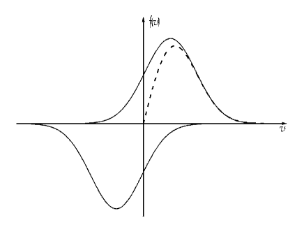
Figure 1: Schematic view of making the Cancelling Jüttner distribution: in the Rest Frame of the Front two Jüttner distributions (full curves) - one with negative velocity, another with positive are subtracted. Dashed curve is the CJ distribution.

The Cancelling Jüttner (CJ) distribution, $f_{CJ}$, is defined by subtracting the ordinary Jüttner distribution (3) with negative velocity, $-v$, from original Jüttner distribution, and and multiplying the obtained result with the step function (figure 1):

$$f_{CJ}=\left(f^{Juttner}_{R}-f^{Juttner}_{L}\right)\Theta(p^{\mu}d\sigma_{\mu})={}$$ (4)

$${=}\frac{\Theta(p^{\mu}d\sigma_{\mu})}{(2\pi\hbar)^{3}}\left(\exp{\frac{\mu{-}p^{\mu}u_{\mu}^{R}}{T}}{-}\exp{\frac{\mu{-}p^{\mu}u_{\mu}^{L}}{T}}\right),$$

Figure 2: The post FO CJ distribution, $f_{CJ}$, in the rest frame of the front (RFF). Baryon mass, $m=1$ GeV, temperature, $T=100$ MeV, density, $n=0.17$ fm^-3 and velocity, $v=0.3$ c in ’A’, $v=0.5$ c in ’B’. The values of each contour are written on the curves. The CJ distribution resembles strongly the post FO distribution obtained in kinetic theory, fig. 2 and 3 in ref. KFOM .

where $u_{\mu}^{R}=(\gamma,\gamma v,0,0)\ \ \textrm{and}\ \ u_{\mu}^{L}=(\gamma,-\gamma v,0,0)$ in the rest frame of the front (RFF). The velocity parameter, $v$, of the CJ distribution is restricted to be positive. When $p^{\mu}d\sigma_{\mu}=0$ the function vanishes at the front, even without step function $\Theta$. The role of the $\Theta(p^{\mu}d\sigma_{\mu})$ part is just to eliminate the negative part of the distibution.

We chose this construction from two Juttner distributions because: 1) It automatically includes the cut, and furthermore a smooth but rapid cut, thus the unrealistic profile of the earlier proposed cut-Juttner distribution Bugaev is not present. 2) It resembles the distribution we obtained from a kinetic model quite well, in any case much better than the cut-Juttner distribution. 3) The formulation is still analytic and not more complicated than the one arising from the cut-Juttner distribution.

Calculations and results will be made in the rest frame of the front (RFF), where the surface element is $d\sigma_{\mu}=(0,1,0,0)d\sigma$. In this frame particles cannot propagate across the front in the negative $x$ direction. We assume that the pre FO side is in thermal equilibrium. If the particle has passed the freeze out layer it cannot scatter back. This layer is idealized as a front or hypersurface. In figure 1, the schematic way of making the CJ distribution is shown. The distribution obtained this way (figure 2) resembles strongly the one obtained numerically in a kinetic FO model KFOM . In the following we demonstrate the use of the Cancelling Jüttner distribution.

III Conservation Laws of Fluid Dynamics

The FO hypersurface is considered to be a discontinuity in space-time, thus instead of derivatives of the discontinuous variables we consider the changes explicitely. We will use the conservation laws of fluid dynamics, but instead of the differential form of continuity equations we have to use comutator form:

$$[N^{\mu}d\sigma_{\mu}]=0\ \ \textrm{and}\ \ [T^{\mu\nu}d\sigma_{\mu}]=0,$$ (5)

where $[A]=A_{1}-A_{0}$, $A_{1}$ is a post FO quantity, and $A_{0}$ is the pre FO quantity. Moreover, entropy across FO hypersurface must not decrease:

$$[S^{\mu}d\sigma_{\mu}]\geq 0.$$ (6)

This condition does not provide additional information about the freezing out matter, but it must be satisfied.

Now our task is to find out the expressions for baryon current, energy-momentum tensor and entropy current in the post FO side. Having these expressions, we will insert them to equations of conservation laws (5), and then we will have a relationship between matter properties in pre and post FO sides. This calculation is straightforward for time-like FO where both the pre- and post FO sides can be characterized as perfect fluids with well defined equation of state and energy-momentum tensor (see ItoRHIC ). In the case of space-like FO with out of equilibrated post FO distribution this calculation has been demonstrated so far only for the cut-Jüttner distribution Anderlik .

The post FO baryon current, $N^{\nu}$, can be calculated inserting the post FO distribution (4) into equation (1). The energy-momentum tensor, $T^{\mu\nu}$, can be obtained in the same way, i.e., inserting the post FO distribution (4) in to the definition:

$$T^{\mu\nu}=\int\frac{d^{3}p}{p^{0}}p^{\mu}p^{\nu}f_{FO}(\vec{r},p;T,n,u^{\mu})$$ (7)

However, we do not have to calculate integral (1) nor (7), but instead we take the already calculated $N^{\mu}$, $T^{\mu\nu}$ and $S^{\mu}$ for the post FO Cut-Jüttner distribution in the reference frame of the gas (RFG), from Anderlik :

$$\begin{array}[]{rl}N^{0}=&\frac{\tilde{n}}{4}\Big{[}vA+a^{2}j[(1+j)K_{2}(a)-\mathcal{K}_{2}(a,b)]+j\frac{b^{3}v^{3}}{3}e^{-b}\Big{]},\\ N^{x}=&\frac{\tilde{n}}{8}\Big{[}(1-v^{2})A-a^{2}e^{-b}\Big{]},\\ T^{00}=&\frac{3\tilde{n}T}{2}\Big{[}j\frac{a^{2}}{2}\Big{(}(1+j)[K_{2}(a)+\frac{a}{3}K_{1}(a)]-\\ -&\mathcal{K}_{2}(a,b)-\frac{a}{3}\mathcal{K}_{1}(a,b)\Big{)}+Bv\Big{]},\\ T^{0x}=&T^{x0}=\frac{3\tilde{n}T}{4}\left[(1-v^{2})B-\frac{a^{2}}{6}(b+1)e^{-b}\right],\\ T^{xx}=&\frac{\tilde{n}T}{2}\left[j\frac{a^{2}}{2}[(1+j)K_{2}(a)-\mathcal{K}_{2}(a,b)]+v^{3}B\right],\\ T^{yy}{=}&T^{zz}{=}\frac{3\tilde{n}T}{4}\Big{[}v(1{-}\frac{v^{2}}{3})B+{\frac{ja^{2}}{3}}\Big{(}(1+j)K_{2}(a)-\\ -&{\cal K}_{2}(a,b)\Big{)}-{\frac{{va^{2}}}{6}}(b{+}1)e^{-b}\Big{]},\\ S^{0}=&\frac{\tilde{n}}{4}\Big{[}(1{-}\frac{\mu}{T})vA+6vB+(1-\frac{\mu}{T})a^{2}j\big{(}(1{+}j)K_{2}(a)-\\ -&{\cal K}_{2}(a,b)\big{)}+ja^{2}\big{(}(1{+}j)K_{1}(a)-{\cal K}_{1}(a,b)\big{)}\Big{]},\\ S^{x}=&\frac{\tilde{n}}{8}\Big{[}(1-v^{2})(1-\frac{\mu}{T})A+6(1-v^{2})B-\\ -&a^{2}(2+b-\frac{\mu}{T})e^{-b}\Big{]},\end{array}$$

where $j=\textrm{sign}(v)$, $\tilde{n}=\pi T^{3}e^{\mu/T}(\pi\hbar)^{-3}$, $\mu$ is chemical potential of the pre FO matter, $a=m/T,\ b=a/\sqrt{1-v^{2}},\ v=d\sigma_{0}/d\sigma_{x},\ A=(2+2b+b^{2})e^{-b},\ B=(1+b+b^{2}/2+b^{3}/6)e^{-b}$ and

$$\mathcal{K}_{n}(a,b)=\frac{2^{n}(n!)}{(2n)!}a^{-n}\int_{b}^{\infty}dx(x^{2}-a^{2})^{n-1/2}e^{-x},$$

i.e. $K_{n}(a)=\mathcal{K}_{n}(a,a)$. All other components of $T^{\mu\nu},N^{\mu}$ and $S^{\mu}$ vanish.

The derivation of $N^{\mu}_{CJ}$ and $T^{\mu\nu}_{CJ}$ will be presented in detail in the mass zero limit in the next section. However, the way of deriving these quantities is the same for both cases: with mass zero limit, or without. The results of $N^{\mu}_{CJ}$, $T^{\mu\nu}_{CJ}$ and $S^{\mu}_{CJ}$ for finite mass $m$, in RFF are:

$$\begin{array}[]{rl}N^{0}_{CJ}=&\gamma\frac{\tilde{n}}{4}\Big{[}3Av-va^{2}e^{-b}-Av^{3}+2a^{2}\Delta_{2}\Big{]},\\ N^{x}_{CJ}=&\gamma\frac{\tilde{n}}{2}\left[a^{2}vK_{2}(a)+j\frac{b^{3}v^{4}}{3}e^{-b}\right],\\ T^{00}_{CJ}=&3\tilde{n}T\gamma^{2}\Big{[}j\frac{a^{2}}{2}\left(\frac{a}{3}\Delta_{1}+(1+\frac{v^{2}}{3})\Delta_{2}\right)+\\ +&B(\frac{v^{5}}{3}-4v^{3}+5v)-va^{2}(b+1)e^{-b}\Big{]},\\ T^{x0}_{CJ}=&T^{0x}_{CJ}=\frac{\tilde{n}T\gamma^{2}a^{2}}{2}\Big{[}4vK_{2}(a)+avK_{1}(a)\Big{]},\\ T^{xx}_{CJ}=&3\tilde{n}T\gamma^{2}\Big{[}j\frac{a^{2}}{2}\left(v^{2}(\Delta_{2}+\frac{a}{3}\Delta_{1})+\frac{1}{3}\Delta_{2}\right)+\\ +&B(-\frac{8}{3}v^{3}+4v)+a^{2}v^{2}(b+1)e^{-b}\Big{]},\\ S^{0}_{CJ}=&\gamma\frac{\tilde{n}}{4}\Big{[}(3v-v^{3})\left((1-\frac{\mu}{T})A+6B\right)+\\ +&2a^{2}j\left((1-\frac{\mu}{T})\Delta_{2}+\Delta_{1}\right)-a^{2}v\left(2+b-\frac{\mu}{T}\right)e^{-b}\Big{]},\\ S^{x}_{CJ}=&\gamma\frac{\tilde{n}}{2}\Big{[}a^{2}K_{2}(a)v(1-\frac{\mu}{T})+a^{2}K_{1}(a)v\Big{]},\end{array}$$

where $\Delta_{i}\equiv K_{i}(a)-\mathcal{K}_{i}(a,b),\ \ i=1,2$ . All other components vanish. From these expressions, one obtains properties of the matter on the post FO side of the FO front.

IV Calculating the Relationship of Matter Properties

Now we will study in more detail the change of matter properties across the FO hypersurface with space-like normal, having local equilibrium in pre FO side, and non-equilibrated matter on the post FO side. In order to connect both sides of the FO hypersurface we will use conservation laws of hydrodynamics.

We are taking baryon current and energy momentum tensor for the cut-Jüttner distribution in the RFG with mass zero limit . Such a approximation is possible when energies are high compared to the masses of particles. From Anderlik $N^{\mu}_{RFG}$ and $T^{\mu\nu}_{RFG}$ read as:

$$N^{0}_{RFG}=\tilde{n}\frac{v+1}{2},\ \ N^{x}_{RFG}=\tilde{n}\frac{1-v^{2}}{4}$$

$$T^{00}_{RFG}=3\tilde{n}T\frac{v+1}{2},\quad T^{0x}_{RFG}=3\tilde{n}T\frac{1-v^{2}}{4},$$

$$T^{xx}_{RFG}=\tilde{n}T\frac{v^{3}+1}{2},\quad T^{zz}_{RFG}=T^{yy}_{RFG}=\frac{T^{00}_{RFG}-T^{xx}_{RFG}}{2}.$$

To get the post FO baryon current and energy-momentum tensor for the CJ distribution in the rest frame of the front (RFF), we are making a Lorentz transformation from the RFG to the RFF of the components of the cut-Jüttner distribution. Thus, we get $N^{\mu}_{RFF}$ and $T^{\mu\nu}_{RFF}$ for the cut-Jüttner distribution in mass zero limit:

$$N^{\mu}_{RFF}=\frac{\tilde{n}\gamma}{4}(-v^{3}+3v+2,v^{2}+2v+1,0,0)$$

$$T^{00}_{RFF}=\frac{\gamma^{2}\tilde{n}T}{4}(v^{5}{-}6v^{3}{+}2v^{2}{+}12v{+}6),$$

$$T^{0x}_{RFF}=T^{x0}_{RFF}=\frac{\gamma^{2}\tilde{n}T}{4}(-v^{4}{+}6v^{2}{+}8v{+}3)$$

$$T^{xx}_{RFF}=\frac{\gamma^{2}\tilde{n}T}{2}(v^{3}{+}3v^{2}{+}3v{+}1),\ \ T^{yy}_{RFF}=T^{zz}_{RFF}=T^{yy}_{RFG}$$

The energy-momentum tensor components $T^{yy}$ and $T^{zz}$ are not changing, because our reference frame is chosen in such a way, that the Lorentz transformation is influencing only time and one spatial component $x$. All other energy-momentum tensor components are equal to zero.

Any of the components presented above for the CJ distribution, for example, $N^{0}_{CJ}$ in the RFF frame, can be found in such a way:

$$N^{0}_{CJ}(v)=N^{0}_{RFF}(v)-N^{0}_{RFF}(-v).$$

This follows from the definition of the CJ distribution function, eq. (4). Thus, the components of the baryon current of the CJ distribution take the form:

$$N^{\mu}_{CJ}=\tilde{n}\gamma\left(\frac{-v^{3}+3v}{2},v,0,0\right),$$ (8)

and the components of the energy-momentum tensor:

$$T^{00}_{CJ}=\tilde{n}T\gamma^{2}(v^{5}{-}3v^{3}{+}6v),\ \ T^{0x}_{CJ}=T^{x0}_{CJ}=4\tilde{n}T\gamma^{2}v,$$ (9)

$$T^{xx}_{CJ}=\tilde{n}T\gamma^{2}(v^{3}{+}3v),\ \ T^{yy}_{CJ}=T^{zz}_{CJ}=\tilde{n}T\frac{{-}v^{3}+3v}{2}.$$ (10)

Now we can introduce flow, particle density, energy density and entropy density for the frozen-out matter. The four-flow of the particles, $u_{\mu}$, can be described in different ways: i) Eckart’s definition:

$$u_{flow,E}^{\mu}=\frac{N^{\mu}_{CJ}}{\sqrt{N^{\nu}_{CJ}N_{\nu,CJ}}},$$ (11)

where the flow $u_{\mu}^{E}$ is tied to conserved particles. ii) Landau’s definition:

$$u_{flow,L}^{\mu}=\frac{T_{CJ}^{\mu\nu}u_{\nu}}{\sqrt{u_{\rho}T^{\rho\nu}_{CJ}u_{\nu}}},$$ (12)

where the flow is tied to energy flow. In case of Cancelling Jüttner distribution there two definitions do not give an identical result, because the CJ distribution is not an equilibrium distribution. In further calculation let us use Eckart’s definition of the flow. Having expression for the flow, we can obtain other macroscopic quantities. Invariant scalar density $n$ is:

$$n=N^{\mu}_{CJ}u_{\mu}^{E}.$$ (13)

Energy density, $e$, and entropy density, $s$, reads as:

$$e^{E}=u_{\mu}^{E}T^{\mu\nu}u_{\nu}^{E},\ \ s^{E}=S^{\mu}u_{\mu}^{E}.$$

Figure 3: The Eckart’s flow velocity, $u$, of the frozen-out particles, described by CJ distribution in RFF, versus velocity parameter of the distribution, $v$.

Figure 4: The proper density of the frozen-out particles, $n$, described by CJ distribution, versus the velocity parameter of the distribution, $v$, with fixed chemical potential, $\mu=10MeV$, and temperature parameter, $T=100MeV$.

As we can see in figure 3, where the flow velocity is plotted versus velocity parameter of the CJ distribution, the Eckart’s flow has the minimum value $0.66c$ in the mass zero limit. Figure 4 shows the post FO density ,$n^{E}$, dependece on velocity parameter, $v$.

V Freeze-out From QGP

We must find expressions for the $N^{\mu}_{0}$ and $T^{\mu\nu}_{0}$ in the pre FO side to use conservation laws (5) across the surface element $d\sigma_{\mu}$. For perfect fluids the energy-momentum tensor (in any reference frame) can be written as ItoRHIC :

$$T^{\mu\nu}=(e+p)u^{\mu}u^{\nu}-pg^{\mu\nu},$$ (14)

where $e$ is the energy density and $p$ is pressure in the local rest (LR) frame. For the baryon current, we use Eckart’s definition for flow: $u^{\mu}=N^{\mu}_{(0)}/\sqrt{N^{\nu}_{(0)}N_{\nu}^{(0)}}$. From this definition follows:

$$N_{(0)}^{\mu}=n_{0}u^{\mu}_{(0)},$$ (15)

where $u^{\mu}_{(0)}=(1,0,0,0)$ and the invariant scalar, $n_{0}=\sqrt{N^{\mu}_{(0)}N_{\mu}^{(0)}}$, is the particle density.

To determine the parameters of the CJ distribution we will use the conservation laws introduced by eq. (5). By using the conservation law for the four-current $[N^{\mu}\ d\sigma_{\mu}]=N^{\mu}_{CJ}d\sigma_{\mu}-N^{\mu}_{(0)}d\sigma_{\mu}^{(0)}=0$, where $d\sigma_{\mu}^{(0)}=\gamma_{0}(v_{0},1,0,0)$ in the pre FO local rest frame, and $d\sigma_{\mu}=(0,1,0,0)$ in the RFF, we get the equation:

$$\tilde{n}\gamma v-n_{0}\gamma_{0}v_{0}=0.$$ (16)

Note that post and pre FO expressions have to be in the same reference frame, in order to use conservation laws correctly. Nevertheless, $N^{\mu}_{0}$ and $d\sigma_{\mu}^{(0)}$ do not have to be transformed to the RFF, because the baryon number crossing the surface is an invariant scalar. However, the energy-momentum current, $T^{\mu\nu}d\sigma_{\mu}$, is not an invariant scalar, thus it must be Lorentz transformed to the RFF. After the transformation $T^{\mu\nu}$ gets a form:

$$T^{\mu\nu}_{(0)RFF}{=}\left(\begin{array}[]{cccc}\gamma^{2}_{0}(e_{0}{+}v^{2}_{0}p_{0})&\gamma^{2}_{0}({-}e_{0}v_{0}{-}p_{0}v_{0})&0&0\\ \gamma^{2}_{0}({-}e_{0}v_{0}{-}p_{0}v_{0})&\gamma^{2}_{0}(e_{0}v_{0}^{2}{+}p_{0})&0&0\\ 0&0&p_{0}&0\\ 0&0&0&p_{0}\\ \end{array}\right).$$

Using the conservation laws for the energy-momentum tensor, $[T^{\mu\nu}\ d\sigma_{\mu}]=T^{\mu\nu}_{CJ}d\sigma_{\mu}-T^{\mu\nu}_{(0)}d\sigma_{\mu}=0$, we obtain two more equations:

$$4\gamma^{2}\tilde{n}Tv-\gamma_{0}^{2}\left(v_{0}e_{0}+v_{0}p_{0}\right)=0$$ (17)

$$\gamma^{2}\tilde{n}T(v^{3}+3v)-\gamma_{0}^{2}\left(v_{0}^{2}e_{0}+p_{0}\right)=0.$$ (18)

Entropy should not decrease, $[S^{\mu}d\sigma_{\mu}]=S^{\mu}_{CJ}d\sigma_{\mu}-S^{\mu}_{(0)}d\sigma_{\mu}^{(0)}\geq 0$, it leads to the condition:

$$\tilde{n}\gamma v\left(1-\frac{\mu}{T}\right)-s_{0}\gamma_{0}v_{0}\geq 0,$$ (19)

which must be satisfied.

The Bag Model Equation of State (EoS) for quark gluon plasma is used to describe the pre FO matter state. It is assumed that quarks and gluons exist in perturbative vacuum, where plasma contains $2(N_{c}^{2}-1)$ gluons and $2N_{c}N_{f}$ quarks ($N_{c}$ and $N_{f}$ are the number of colors and number of flavors) Sh80 . The Bag Model EoS is based on Stefan-Boltzmann EoS, including a bag constant $B$. From ItoRHIC pre FO quantities are expressed as:

$$e_{0}=\left(\frac{37}{30}\pi^{2}T_{0}^{4}+\frac{1}{3}\mu^{2}T_{0}^{2}+\frac{1}{54\pi^{2}}\mu^{4}+\Lambda_{B}^{4}\right)\frac{1}{(\hbar c)^{3}}$$

$$n_{0}=\frac{2}{9}\left(\mu^{2}T_{0}^{2}+\frac{1}{9\pi^{2}}\mu^{3}\right)\frac{1}{(\hbar c)^{3}}$$

$$s_{0}=\left(\frac{74}{45}\pi^{2}T_{0}^{3}+\frac{2}{9}\mu^{2}T_{0}^{2}\right)\frac{1}{(\hbar c)^{3}}$$

$$p_{0}=\frac{e_{0}}{3}-\frac{4}{3}B,\quad\textrm{where}\quad B=\frac{\Lambda_{B}^{4}}{(\hbar c)^{3}}.$$

Here $\mu$ is baryon chemical potential.

Using above and equations (16 - 18) we can evaluate how post FO matter properties depend on the pre FO side matter properties. It is enough to fix four quantities in the Bag Model EoS to obtain the properties of the post FO matter. To describe the pre FO side we will use: initial temperature, $T_{0}$, bag constant, $\Lambda_{B}$, initial baryon density, $n_{0}$, and initial velocity, $v_{0}$, to have pre FO energy density, pressure, entropy density and baryon chemical potential.

Nevertheless, the CJ distribution has a negative aspect: not for all initial values it is possible to calculate post FO matter parameters. There are two reasons: 1. Entropy must not decrease, 2. The maximum of the Jüttner distribution function must be on the positive velocity side. When maximum of the Jüttner distribution is at velocity zero ($f_{Juttner}(v=0)|_{RFF}=\max{f_{Juttner}(v)|_{RFF}}$), the CJ distribution is a ’zero’ function ($f_{CF}(v){=}0,\forall\ v$). This problem depends on how pre FO properties such as velocity, $v_{0}$, density, $n_{0}$, bag constant, $\Lambda_{B}$, and initial temperature, $T_{0}$, are chosen.

Figure 5: The boundaries of the pre FO density, $n_{0}$, and velocity, $v_{0}$, to have correct post FO distribution function, $f_{CJ}$, in the rest frame of the front (RFF) with fixed initial temperature, $T_{0}$, and bag constant, $\Lambda_{B}$. The CJ distribution is applicable for initial conditions which are to the right from the curves, i.e. for large flow velocities in RFF.

The boundary conditions for pre FO velocity, $v_{0}$ and density, $n_{0}$, with fixed bag constant, $\Lambda_{B}$, and initial temperature, $T_{0}$, are shown in figure 5. Such a conditions for the pre FO matter, which are to the right from the curves in figure 5, have to be satisfied for the CJ distribution because we are dealing with a FO hypersurface with space-like normal. The shape of the curves are influenced by the way of making the CJ distribution i.e. when the post FO velocity becomes imaginary. The cutoff of the curves is influenced by the entropy condition. In order to have perspicuity we compare two curves: one with initial temperature $T_{0}=60$ MeV, another with $T_{0}=100$ MeV ($\Lambda_{B}=200$ MeV for both curves). Having higher temperature, the density (or velocity) can be lower than in the lower temperature case. On the other hand, to insure the entropy condition, the density in the higher temperature case must be higher (more than $0.5$ fm^-3) than in the case of lower temperature, where it must be just more than $0.1$ fm^-3. Temperature is influencing the length of the curve and moves it to the left when temperature increases, and bag constant is changing the gradient of the curve in the $v_{0},n_{0}$ plane.

Now, having boundary conditions we can start calculating matter properties of the post FO side. From equations (16 - 18) we get one equation for the post FO velocity parameter:

$$v=\sqrt{\frac{4(v_{0}^{2}e_{0}+p_{0})}{v_{0}(e_{0}+p_{0})}-3}.$$

Note, that post FO velocity, $v$, temperature, $T$, and density, $\tilde{n}$, are not physical quantities - they are parameters of the CJ distribution.

Figure 6: Change of the velocity parameter across the FO hypersurface, in RFF, described by the CJ distribution for the different initial parameters: 1. $n_{0}=0.5$ fm^-3, $\Lambda_{0}=150$ MeV full curve; 2. $n_{0}=1$ fm^-3, $\Lambda_{0}=200$ MeV dashed curve; 3. $n_{0}=0.2$ fm^-3, $\Lambda_{0}=150$ MeV dotted curve and $T_{0}=60$ MeV for all curves.

As we see in figure 6 the post FO velocity parameter is all the time smaller than the pre FO velocity.

Figure 7: The dependence of the post FO baryon flow on the pre FO velocity for the different initial parameters: 1. $n_{0}=0.5$ fm^-3, $\Lambda_{0}=150$ MeV full curve; 2. $n_{0}=1$ fm^-3, $\Lambda_{0}=200$ MeV dashed curve; 3. $n_{0}=0.2$ fm^-3, $\Lambda_{0}=150$ MeV dotted curve and $T_{0}=60$ MeV for all curves.

The post FO flow velocity, $u_{flow}$, is calculated using Eckart’s definition of the flow using formula (11). Figure 7 shows the post FO baryon flow velocity dependence on the pre FO velocity, $v_{0}$. We observe, that the flow does not decrease in the same way as the post FO velocity parameter, $v$. Only in the case of low initial density ($n_{0}=0.2$ fm^-3 in figure 7) we have decrease of velocity going from pre to post FO side. To calculate the final baryon density we are using the equation (13), which can be rewritten for the case of Eckart’s flow:

$$n=\sqrt{N^{\mu}_{CJ}N_{\mu,CJ}}.$$

Figure 8: The change of the baryon density across the FO hypersurface for different initial parameters: 1. $v_{0}=0.6$ c, $\Lambda_{0}=150$ MeV full curve; 2. $v_{0}=0.6$ c, $\Lambda_{0}=200$ MeV dashed curve; 3. $v_{0}=0.5$ c, $\Lambda_{0}=200$ MeV dotted curve and $T_{0}=60$ MeV for all curves.

From the results presented in the figure 8 it is seen that the baryon charge density in the post FO side is decreasing compared to the density in the pre FO side. The two lines are parallel to each other if initial velocity, $v_{0}$, and initial temperature, $T_{0}$, are the same.

VI Conclusions

We have studied the problem of negative contribution in the Cooper-Frye (2) formula for the 3-dimentional hypersurface with space-like normal. The Cancelling Jüttner distribution function was suggested as a solution for this problem. We have showed the applicability and properties of the CJ distribution by using the Bag Model equation of state for QGP and conservation laws of hydrodynamics across the FO hypersurface.

The CJ distribution solves the problem of negative contribution in the Cooper-Frye formula and has a physical form unlike the cut-Jüttner distribution. In future studies one should analyze, if the conditions of applicability of CJ distribution are satisfied in space-like hypersurfaces obtained from hydrodynamical calculations.

It will be interesting to see how large corrections this procedure will give to the results obtained from simple Cooper-Frye description.

References

• (1) F. Cooper, G. Frye, Phys. Rew. D 10, (1974) 186
• (2) F. Jüttner, Ann. Phys und Chemie, 34, 856 (1911)
• (3) Cs. Anderlik, L.P. Csernai, F. Grassi, W. Greiner, Y. Hama, T. Kodama, Zs.I. Lazar, V.K. Magas, H.Stöcker, Phys. Rev. C 59 (1999) 3309, (nucl-th/9806004)
• (4) K.A. Bugaev, Nucl. Phys. A606 (1996) 559
• (5) V.K. Magas, Cs. Anderlik, L.P. Csernai, F. Grassi, W. Greiner, Y. Hama, T. Kodama, Zs. Lazar and H. Stöcker, Heavy Ion Phys. 9 (1999) 193, (nucl-th/9903045)
• (6) L.P. Csernai, Introduction to Relativistic Heavy Ion Phys. (1999)Heavy Ion Collisions John Wiley Ltd, (1994)
• (7) L.D. Landau and E.M. Lifsitz Classical Field Theory Nauka, Moscow, (1973)
• (8) E.V. Shuryak Phys.Rep. 61, 71, (1980)