MASSIVE PARTICLE DECAY AND
COLD DARK MATTER ABUNDANCE

Abstract

    The decoupling of a cold relic, during a decaying-particle-dominated cosmological evolution is analyzed, the relic density is calculated both numerically and semi-analytically and the results are compared with each other. Using plausible values (from the viewpoint of supersymmetric models) for the mass and the thermal averaged cross section times the velocity of the cold relic, we investigate scenaria of equilibrium or non-equilibrium production. In both cases, acceptable results for the dark matter abundance can be obtained, by constraining the reheat temperature of the decaying particle, its mass and the averaged number of the produced cold relics. The required reheat temperature is, in any case, lower than about $20~{}{\rm GeV}$.

Keywords: Cosmology, Dark Matter
PACS codes: 98.80.Cq, 95.35.+d

Published in Astropart. Phys. 21, 689 (2004)

1 INTRODUCTION

The enigma of the Cold Dark Matter (CDM) constitution of the universe becomes more and more precisely defined, after the recently announced WMAP results [1, 2], which determine the CDM abundance, $\Omega_{\rm CDM}h^{2}$, with an unprecedented accuracy:

$$\Omega_{\rm CDM}h^{2}=0.1126_{-0.0181}^{+0.0161}$$ (1)

at $95\%$ confidence level. In light of this, the relic density of any CDM candidate $\tilde{\chi}$ (i.e, which decouples being non relativistic), $\Omega_{\tilde{\chi}}h^{2}$, is to satisfy a very narrow range of values:

$${\sf(a)}~{}~{}0.09\lesssim\Omega_{\tilde{\chi}}h^{2}~{}~{}\quad\mbox{and}\quad~{}~{}{\sf(b)}~{}~{}\Omega_{\tilde{\chi}}h^{2}\lesssim 0.13$$ (2)

which tightly restricts the parameter space of the theories which support the existence of $\tilde{\chi}$. The most popular of these are the $R$-parity conserving supersymmetric (SUSY) theories which identify $\tilde{\chi}$ to the stable lightest SUSY particle (LSP) [3]. According to the standard scenario, (i) $\tilde{\chi}$ decouples from the cosmic fluid during the radiation-dominated (RD) era, (ii) being in chemical equilibrium with plasma and (iii) produced through thermal scatterings in the plasma. The condition (ii) is satisfied naturally by the lightest neutralino of the minimal SUSY standard model (MSSM), which turns out to have the required strength of interactions, being weakly interacting.

Although quite compelling, this scenario comes across with difficulties, especially when it is applied in the context of economical and predictive versions of MSSM. E.g., in most of the parameter space of the Constrained MSSM (CMSSM) [4], $\tilde{\chi}$ turns out to be bino and its $\Omega_{\tilde{\chi}}h^{2}$ exceeds the bound of Eq. (2b). Several suppression mechanisms of $\Omega_{\tilde{\chi}}h^{2}$ have been proposed so far: Bino-sleptons [5] and particularly, for large $\tan\beta$, bino-stau [6], bino-stops [7, 8] or bino-chargino [9] coannihilations and/or A-pole effect [10] can efficiently reduce $\Omega_{\tilde{\chi}}h^{2}$. Also several kinds of non-universality in the Higgs [11] and/or gaugino [12, 13] and/or sfermionic sector [14] can help in the same direction, creating additional coannihilation effects. As is expected, a more or less tuning of the SUSY parameters is needed in these cases, without a simultaneous satisfaction of other phenomenological constraints to be always possible (see, e.g. Ref. [2]). On the other hand, $\Omega_{\tilde{\chi}}h^{2}$ turns out to be lower than the bound of Eq. (2a) in other models, e.g., in the anomaly mediated SUSY breaking model (AMSBM) where $\tilde{\chi}$ is mostly wino [15] or in models based on $SU(5)$ gaugino non-universality [16], where $\tilde{\chi}$ can be higgsino. Then we have to invoke another CDM candidate [17], in order for the range of Eq. (2) to be fulfilled.

However, this picture can dramatically change, if the standard assumption (i) is lifted. Indeed, since there is no direct information for the history of the Cosmos before the epoch of nucleosynthesis (i.e., temperatures $T>1~{}{\rm MeV}$) the decoupling of $\tilde{\chi}$ can occur not in the RD era. As was pointed out a lot years ago [18] and, also, recently [19, 20], the ${\tilde{\chi}}$ decoupling can be related to the decay of a massive scalar particle. The modern cosmo-particle theories are abundant in such fields, e.g. inflatons [21, 22, 23, 24], dilatons or moduli [25, 26], Polonyi field [27], $q$-balls [28] (see, also [29]). During their decay, these particles perform coherent oscillations “reheating” the universe [30]. This phenomenon is not instantaneous [31, 21]. In particular, the maximum temperature during this period is much larger than the so-called reheat temperature, which can be better considered as the largest temperature of the RD era [19]. Consequently, the “freeze out” of $\tilde{\chi}$ could be realized before the completion of the reheating. The cosmological evolution during this phase is strongly modified as regards the standard one [30], with crucial consequences to $\Omega_{\tilde{\chi}}h^{2}$ calculation [19, 20, 26, 32]. Namely, two types of $\tilde{\chi}$-production emerge, in contrast with (ii): The chemically equilibrium (EP) and the non-equilibrium production (non-EP) (in both cases, kinetic equilibrium of $\tilde{\chi}$’s is assumed [19]). In this paper we extend the analysis in Ref. [19], lifting also the assumption (iii) of the standard scenario: We include the possibility (which, naturally arises even without direct coupling [23, 24]) that the decaying particle can decay to $\tilde{\chi}$. The problem has already been faced semi-quantitatively in Refs [26, 32, 23, 24] and numerically in Ref. [33] for significantly more massive $\tilde{\chi}$’s.

Our numerical and semi-analytical analyses are exposed in secs 2 and 3. The obtained results are compared with each other in sec. 4. There, we realize, also, a model independent application of our findings in the case of SUSY models inspired ${\tilde{\chi}}$ masses and cross sections. We find that comfortable satisfaction of Eq. (2) can be achieved, by constraining the reheat temperature to rather low values, the mass of the decaying particle and the averaged number of the produced $\tilde{\chi}$’s, without any tuning of the SUSY parameters.

Throughout the text and the formulas, brackets are used by applying disjunctive correspondence and natural units ($\hbar=c=k_{B}=1$) are assumed.

2 DYNAMICS OF MASSIVE PARTICLE DECAY

We consider a scalar particle $\phi$ with mass $m_{\phi}$, which decays with a rate $\Gamma_{\phi}$ into radiation, producing an average number $N_{\tilde{\chi}}$ of $\tilde{\chi}$’s with mass $m_{\tilde{\chi}}$, rapidly thermalized. We, also, let open the possibility (contrary to Ref. [26]) that ${\tilde{\chi}}$’s are produced through thermal scatterings in the bath. Our theoretical analysis is presented in sec. 2.1 and its numerical treatment in sec. 2.2. Useful approximated expressions are derived in sec. 2.3.

2.1 RELEVANT BOLTZMANN EQUATIONS

The energy density of radiation $\rho_{{}_{\rm R}}$ and the number densities of $\phi$, $n_{\phi}$, and $\tilde{\chi}$, $n_{\tilde{\chi}}$, satisfy the following Boltzmann equations [21, 26] (we use the shorthand $\Delta_{\phi}=(m_{\phi}-N_{\tilde{\chi}}m_{\tilde{\chi}})/m_{\phi}$):

$$\dot{n}_{\phi}+3Hn_{\phi}+\Gamma_{\phi}n_{\phi}=0,$$ (3)

$$\dot{\rho}_{{}_{\rm R}}+4H\rho_{{}_{\rm R}}-\Gamma_{\phi}\Delta_{\phi}m_{\phi}n_{\phi}-2m_{\tilde{\chi}}\langle\sigma v\rangle\left(n_{\tilde{\chi}}^{2}-n_{\tilde{\chi}}^{\rm eq2}\right)=0,$$ (4)

$$\dot{n}_{\tilde{\chi}}+3Hn_{\tilde{\chi}}+\langle\sigma v\rangle\left(n_{\tilde{\chi}}^{2}-n_{\tilde{\chi}}^{\rm eq2}\right)-\Gamma_{\phi}N_{\tilde{\chi}}n_{\phi}=0,$$ (5)

where dot stands for derivative with respect to (w.r.t) the cosmic time $t$, $\langle\sigma v\rangle$ is the thermal-averaged cross section of $\tilde{\chi}$ particles times velocity and $H$ the Hubble expansion parameter which is given by ($M_{\rm P}=1.22\times 10^{19}~{}{\rm GeV}$ is the Planck scale):

$$H^{2}=\frac{8\pi}{3M_{\rm P}^{2}}\left(\rho_{\phi}+\rho_{{}_{\rm R}}+\rho_{\tilde{\chi}}\right),\quad\mbox{with}\quad\rho_{\phi}=\Delta_{\phi}m_{\phi}n_{\phi}\quad\mbox{and}\quad\rho_{\tilde{\chi}}=m_{\tilde{\chi}}n_{\tilde{\chi}}.$$ (6)

The equilibrium number density of $\tilde{\chi}$, $n_{\tilde{\chi}}^{\rm eq}$ obeys the Maxwell-Boltzmann statistics:

$$n_{\tilde{\chi}}^{\rm eq}(x)=\frac{g}{(2\pi)^{3/2}}m_{\tilde{\chi}}^{3}\>x^{3/2}\>e^{-1/x}P_{2}(1/x),\quad\mbox{where}\quad x=T/m_{\tilde{\chi}},$$ (7)

$g=2$ is the number of degrees of freedom of ${\tilde{\chi}}$ and $P_{n}(z)=1+(4n^{2}-1)/8z$ is obtained by asymptotically expanding the modified Bessel function of the second kind of order $n$.

The temperature, $T$, and the entropy density, $s$, can be found using the relations:

$$\mbox{\sf(a)}~{}~{}\rho_{{}_{\rm R}}=\frac{\pi^{2}}{30}g_{\rho*}\ T^{4}\quad\mbox{and}\quad\mbox{\sf(b)}~{}~{}s=\frac{2\pi^{2}}{45}g_{s*}\ T^{3},$$ (8)

where $g_{\rho*}(T)~{}[g_{s*}(T)]$ are the energy [entropy] effective number of degrees of freedom at temperature $T$. Their numerical values are evaluated by using the tables included in micrOMEGAs [34], originated from the DarkSUSY package [35].

Central role to our investigation plays the reheat temperature. Its precise value, $T_{\rm rh}$, can be found, by solving numerically the following [36]:

$$\rho_{{}_{\rm R}}(T_{\rm rh})=\rho_{\phi}(T_{\rm rh}).$$ (9)

However, following Ref. [19], we prefer to handle reheat temperature as an input parameter, $T_{\rm RH}$, defining it through an analytic formula, which, however approximates fairly (within 10$\%$) $T_{\rm rh}$. This can be expressed in terms of $\Gamma_{\phi}$, using the following [31, 36]:

$$\Gamma_{\phi}=4\sqrt{\frac{\pi^{3}g_{\rho*}(T_{\rm RH})}{45}}\frac{T_{\rm RH}^{2}}{M_{\rm P}}\cdot$$ (10)

Eq. (10) is derived consistently with Eq. (18) and differs from the corresponding definition in Ref. [19] by a factor 2 (our choice is justified in sec. 4.1).

2.2 NUMERICAL INTEGRATION

The numerical integration of Eqs (3)–(5) is facilitated by absorbing the dilution terms. To this end, we convert the time derivatives to derivatives w.r.t the scale factor, $R$ [21, 19]. We find it convenient to define the following dimensionless variables:

$$f_{\phi}=n_{\phi}R^{3},\quad f_{\rm R}=\rho_{{}_{\rm R}}R^{4}\quad\mbox{and}\quad f_{\tilde{\chi}}^{[\rm eq]}=n^{[\rm eq]}_{\tilde{\chi}}R^{3}\ .$$ (11)

In terms of these variables, Eqs (3)–(5) become:

$$\frac{df_{\phi}}{dR} = -\Gamma_{\phi}\frac{f_{\phi}}{HR},$$ (12)

$$\frac{df_{\rm R}}{dR} = \Gamma_{\phi}\Delta_{\phi}m_{\phi}\frac{f_{\phi}}{H}+2m_{\tilde{\chi}}\langle\sigma v\rangle\frac{f_{\tilde{\chi}}^{2}-f_{\tilde{\chi}}^{\rm eq2}}{HR^{3}},$$ (13)

$$\frac{df_{\tilde{\chi}}}{dR} = -\langle\sigma v\rangle\frac{f_{\tilde{\chi}}^{2}-f_{\tilde{\chi}}^{\rm eq2}}{HR^{4}}+\Gamma_{\phi}N_{\tilde{\chi}}\frac{f_{\phi}}{HR},$$ (14)

where

$$H=\sqrt{\frac{8\pi}{3}}\frac{R^{-3/2}}{M_{\rm P}}\left(\Delta_{\phi}m_{\phi}f_{\phi}+f_{\rm R}/R+m_{\tilde{\chi}}f_{\tilde{\chi}}\right)^{1/2}\ .$$ (15)

Since at early times the energy density of the universe is completely dominated by this of $\phi$ field, $m_{\phi}n_{{}_{\rm I}}$, the system of Eqs (12)–(14) is solved, imposing the following initial conditions:

$$f_{\phi}(R_{\rm I})=n_{{}_{\rm I}}R^{3}_{\rm I}\quad\mbox{and}\quad f_{\rm R}(R_{\rm I})=f_{\tilde{\chi}}(R_{\rm I})=0,\quad\mbox{with}\quad R_{\rm I}=m_{\phi}^{-1}\ .$$ (16)

2.3 SEMI-ANALYTICAL APPROACH

We can obtain a comprehensive and rather accurate approach of the dynamics of the decaying-particle-dominated cosmology, following the arguments of Ref. [19]. At the epoch before the completion of reheating, $T\gg T_{\rm RH}$, the universe is dominated by the number density of $\phi$ which initially has a large value $n_{{}_{\rm I}}$. Its evolution is given by the exact solution of Eq. (3) [30, 31, 36], which at early times, can be written as:

$$n_{\phi}=n_{{}_{\rm I}}\left(\frac{R}{R_{\rm I}}\right)^{-3}.$$ (17)

Inserting this into Eq. (6), we obtain:

$$H^{2}=H_{\rm I}^{2}\left(\frac{R}{R_{\rm I}}\right)^{-3},\quad\mbox{with}\quad H^{2}_{\rm I}=\frac{8\pi}{3M_{P}^{2}}\Delta_{\phi}m_{\phi}n_{{}_{\rm I}}.$$ (18)

At early times the last term of the left part side of Eq. (13) can be safely ignored and it can be easily solved, after substituting Eqs (17) and (18) in it, with result:

$$f_{\rm R}=\frac{2}{5}f_{\rm Rc}\ R_{\rm I}^{3/2}\left(R^{5/2}-R_{\rm I}^{5/2}\right),\quad\mbox{with}\quad f_{\rm Rc}=\Gamma_{\phi}\Delta_{\phi}H_{\rm I}^{-1}m_{\phi}n_{{}_{\rm I}}.$$ (19)

Combining Eqs (19) and (8a), we end up with the following relation:

$$T=\left(\frac{12}{\pi^{2}g_{\rho*}}f_{\rm Rc}\right)^{1/4}\left(\left(\frac{R}{R_{\rm I}}\right)^{-3/2}-\left(\frac{R}{R_{\rm I}}\right)^{-4}\right)^{1/4}\cdot$$ (20)

The function $T(R/R_{\rm I})$ reaches at (see Fig. 2.3)

$$\left(\frac{R}{R_{\rm I}}\right)_{0}=1.48,\quad\mbox{a maximum value}\quad T_{\rm max}=0.767\left(\frac{12}{\pi^{2}g_{\rho*}}f_{\rm Rc}\right)^{1/4}\cdot$$ (21)

[l] The evolution of $x=T/m_{\tilde{\chi}}$ versus $R/R_{\rm I}$, derived from the numerical solution of Eqs (3)–(5) (solid lines), from Eq. (20) (crosses) and from Eq. (22) (open circles) for the parameters of Fig. 2-${\sf(a~{}[b])}$ (normal [light] grey lines, crosses, circles).

For $T<T_{\rm max}$ the second term in the second parenthesis in Eq. (20) can be eliminated. From the resulting expression, we can derive the following useful relations, which “signalize” the deviation from the standard RD evolution. Namely:

$\bullet$ Scale factor-temperature relation:

$$g_{\rho*}^{2/3}\ R\ T^{8/3}=\left(\frac{12}{\pi^{2}}f_{\rm Rc}\right)^{2/3}R_{\rm I}.$$ (22)

Recall that in the RD period is the quantity $g^{1/3}_{s*}(T)RT$ which remains constant.

$\bullet$ Expansion rate-temperature relation:

$$H=\frac{\pi^{2}}{12}\ g_{\rho*}\ f^{-1}_{\rm Rc}\ H_{\rm I}\ T^{4}\,,~{}~{}~{}~{}$$ (23)

which is obtained by solving Eq. (22) w.r.t $R$ and inserting it into Eq. (18). Note that during the RD phase, $H$ is proportional to $T^{2}$ and not to $T^{4}$.

In Fig. 1, we show $x=T/m_{\tilde{\chi}}$ as a function of $R/R_{\rm I}$ for the case of two representative examples which will be analyzed in sec. 4.1. The solid lines are obtained by using Eq. (8a) and the precise numerical solution of Eqs (3)–(5), whereas crosses [open circles] are from the approximated Eq. (20 [22]). Good agreement is observed for $T_{\rm max}>T>T_{\rm RH}$ in both cases.

3 COLD DARK MATTER ABUNDANCE

The aim of this section is the calculation of $\Omega_{\tilde{\chi}}h^{2}$ based on the already obtained semi-analytical expressions. We assume that $\tilde{\chi}$’s are non-relativistic around the ‘critical’ temperatures $T_{\ast}$ or $T_{\rm F}$ (see below) and never in chemical equilibrium after the completion of reheating (however, see sec. 3.4). The relevant Boltzmann equation is properly re-formulated in sec. 3.1. Then two cases are investigated: $\tilde{\chi}$’s do (sec. 3.3) or do not reach (sec. 3.2) chemical equilibrium with plasma. The condition which discriminates the two possibilities is specified in sec. 3.2.

3.1 REFORMULATION OF THE BOLTZMANN EQUATION

Our first step is the re-expression of Eq. (5) in terms of the variables $Y^{\rm[eq]}=n^{\rm[eq]}_{\tilde{\chi}}/s^{8/3}$ in order to absorb the dilution term. Armed with Eqs (22) and (23), we are able now to convert the derivatives w.r.t $t$, to derivatives w.r.t $x=T/m_{\tilde{\chi}}$. In fact, supposing that $g_{s*}(T)$ and $g_{\rho*}(T)$ vary very little from their values at $T_{\rm RH}$ and differentiating the constant quantity $Rs^{8/9}$ (see Eq. (22) and (8b)) w.r.t $t$, we obtain:

$$-8\dot{s}=9Hs\Rightarrow\dot{x}^{-1}=-8s^{\prime}/9Hs,$$ (24)

where prime means derivative w.r.t $x$. Hence, Eq. (5) can be rewritten in terms of the new variables as:

$$\dot{Y}=-\langle\sigma v\rangle\>\left(Y^{2}-{Y^{\rm eq}}^{2}\right)s^{8/3}+\Gamma_{\phi}N_{\tilde{\chi}}n_{\phi}s^{-11/3}.$$ (25)

Replacing $R$ by $x$ in Eq. (17), through Eq. (22), we arrive at:

$$n_{\phi}(x)=n_{{}_{\rm I}}(x/x_{{}_{\rm I}})^{8},$$ (26)

with $x_{{}_{\rm I}}=T_{\rm I}/m_{\tilde{\chi}}$ and $T_{\rm I}$ the temperature corresponding to $R_{\rm I}$ derived from Eq. (22). Differentiating Y w.r.t $x$ and replacing $\dot{x}^{-1}$ by Eq. (24), we obtain:

$$Y^{\prime}=\dot{Y}\dot{x}^{-1}\Rightarrow Y^{\prime}=-\frac{8s^{\prime}}{9sH}m_{\tilde{\chi}}\dot{Y}.$$ (27)

Substituting Eqs (8b), (23) and (25) in Eq. (27), this reads:

$$Y^{\prime}=y_{{}_{n}}\left(Y^{2}-Y^{\rm eq2}\right)x^{3}-y_{{}_{N}}x^{-5},$$ (28)

where $$y_{{}_{n}}(x)=\frac{64}{45}\left(\frac{2\pi^{2}}{45}\right)^{5/3}H_{\rm I}^{-1}f_{\rm Rc}\ m^{4}_{\tilde{\chi}}\ g_{\rm ol}\ \langle\sigma v\rangle$$ (29)

and $$y_{{}_{N}}(x)=\frac{64}{45}\left(\frac{2\pi^{2}}{45}\right)^{-11/3}H_{\rm I}^{-1}\ N_{\tilde{\chi}}\ \Gamma_{\phi}\ f_{\rm Rc}\ n_{{}_{\rm I}}\ x_{{}_{\rm I}}^{-8}m^{-12}_{\tilde{\chi}}\bar{g}_{\rm ol}.$$ (30)

The shorthand $g_{\rm ol}=g_{\rho*}^{-1/2}\ g_{s*}^{5/3}\ g_{*}^{1/2}$ and $\bar{g}_{\rm ol}=g_{\rho*}^{-1/2}\ g_{s*}^{-11/3}\ g_{*}^{1/2}$ has been used, with [12]:

$$g_{*}^{1/2}=\frac{g_{s*}}{\sqrt{g_{\rho*}}}\left(1+\frac{xg^{\prime}_{s*}}{3g_{s*}}\right)\cdot$$

3.2 NON-EQUILIBRIUM PRODUCTION

In this case, $Y\ll Y^{\rm eq}$ and so, $Y^{2}-Y^{\rm eq2}\simeq-Y^{\rm eq2}$. Inserting this into Eq. (28) and integrating from $x_{{}_{\rm I}}$ down to $x_{{}_{\rm RH}}=T_{\rm RH}/m_{\tilde{\chi}}$, we arrive at $Y(x_{{}_{\rm RH}})=Y_{\rm RH}$:

$$Y_{\rm RH}=Y_{n}(x_{{}_{\rm RH}})+Y_{N}(x_{{}_{\rm RH}}),$$ (31)

with $$Y_{n}(x)=\frac{64}{45}\frac{g^{2}}{(2\pi)^{3}}\left(\frac{2\pi^{2}}{45}\right)^{-11/3}H_{\rm I}^{-1}\ f_{\rm Rc}\ J_{n}(x)\ m_{\tilde{\chi}}^{-6}$$ (32)

and $$Y_{N}(x)=\frac{64}{45}\left(\frac{2\pi^{2}}{45}\right)^{-11/3}H_{\rm I}^{-1}\ N_{\tilde{\chi}}\ \Gamma_{\phi}\ J_{N}(x)\ f_{\rm Rc}\ m_{\tilde{\chi}}^{-12}\ n_{{}_{\rm I}}\ x_{{}_{\rm I}}^{-8}\ ,$$ (33)

where we have defined the quantities ($x_{{}_{\rm I}}$ can be approximated by infinity, since $x_{{}_{\rm I}}\gg x_{{}_{\rm RH}}$):

$$J_{n}(x^{\prime})=\int_{x^{\prime}}^{\infty}dx\ x^{-10}e^{-2/x}P^{2}_{2}(1/x)g_{s*}^{-16/3}g_{\rm ol}\langle\sigma v\rangle\ \quad\mbox{and}\quad J_{N}(x^{\prime})=\int_{x^{\prime}}^{\infty}dx\ x^{-5}\bar{g}_{\rm ol}\ .$$ (34)

The maximum $\tilde{\chi}$ particles production takes place at $x_{\ast}=T_{\ast}/m_{\tilde{\chi}}$ (=0.212, for constant $\langle\sigma v\rangle$), where the integrand of $J_{n}$ reaches its maximum [19]. Therefore, the condition which discriminates the EP from the non-EP of $\tilde{\chi}$’s:

$$Y_{n}(x_{\ast})+Y_{N}(x_{\ast})-Y^{\rm eq}(x_{\ast})\left\{\matrix{<0\hfill,&\mbox{non-EP}\hfill\cr\geq 0\hfill,&\mbox{EP}\hfill\cr}\right.$$ (35)

3.3 EQUILIBRIUM PRODUCTION

In this case, we introduce the notion of freeze out temperature, $T_{\rm F}=x_{{}_{\rm F}}m_{\tilde{\chi}}$ [31, 37], which assists us to study Eq. (28) in the two extreme regimes:

$\bullet$ At very early times, when $x\gg x_{{}_{\rm F}}$, $\tilde{\chi}$’s are very close to equilibrium. So, it is more convenient to rewrite Eq. (28) in terms of the variable $\Delta(x)=Y(x)-Y^{\rm eq}(x)$ as follows:

$$\Delta^{\prime}=-{Y^{\rm eq}}^{\prime}+y_{{}_{n}}\Delta\left(\Delta+2Y^{\rm eq}\right)\ x^{3}-y_{{}_{N}}\ x^{-5}.$$ (36)

The freeze-out temperature can be defined by

$$\Delta(x_{{}_{\rm F}})=\delta_{\rm F}\>Y^{\rm eq}(x_{{}_{\rm F}})\Rightarrow\Delta(x_{{}_{\rm F}})\Big{(}\Delta(x_{{}_{\rm F}})+2Y^{\rm eq}(x_{{}_{\rm F}})\Big{)}=\delta_{\rm F}(\delta_{\rm F}+2)\ Y^{\rm eq2}(x_{{}_{\rm F}}),$$ (37)

where $\delta_{\rm F}$ is a constant of order one determined by comparing the exact numerical solution of Eq. (28) with the approximate under consideration one. Inserting Eqs (37) into Eq. (36) and neglecting $\Delta^{\prime}$ (since $\Delta^{\prime}\ll{Y^{\rm eq}}^{\prime}$), we obtain the following equation, which can be solved w.r.t $x_{{}_{\rm F}}$ iteratively:

$$\Big{(}\ln Y^{\rm eq}(x_{{}_{\rm F}})\Big{)}^{\prime}=y_{{}_{n{\rm F}}}\delta_{\rm F}(\delta_{\rm F}+2)Y^{\rm eq}(x_{{}_{\rm F}})x_{{}_{\rm F}}^{3}-y_{{}_{N{\rm F}}}x_{{}_{\rm F}}^{-5}/Y^{\rm eq}(x_{{}_{\rm F}}),\quad\mbox{with}$$ (38)

$$y_{{}_{N[n]\rm F}}=y_{{}_{N[n]}}(x_{{}_{\rm F}})\quad\mbox{and}\quad\Big{(}\ln Y^{\rm eq}(x)\Big{)}^{\prime}=\frac{1}{x^{2}}-\frac{13}{2x}-\frac{8g^{\prime}_{s*}}{3g_{s*}}-\frac{P^{\prime}_{2}(1/x)}{x^{2}P_{2}(1/x)}\cdot$$ (39)

$\bullet$ At late times, when $x\ll x_{{}_{\rm F}}$, $Y\gg Y^{\rm eq}$ and so, $Y^{2}-Y^{\rm eq2}\simeq Y^{2}$. Inserting this into Eq. (28), the value of $Y$ at $T_{\rm RH}$, $Y_{\rm RH}=Y(x_{{}_{\rm RH}})$ can be found by solving the resulting differential equation. We distinguish the cases:

i. For $N_{\tilde{\chi}}=0$, the integration from $x_{{}_{\rm F}}$ down to $x_{{}_{\rm RH}}$ can be made trivially, with result:

$$Y_{\rm RH}=\left(\frac{1}{Y_{\rm F}}+\frac{8}{15\pi}\left(\frac{2\pi^{2}}{45}\right)^{5/3}M_{\rm P}^{2}\>\Gamma_{\phi}\>m_{\tilde{\chi}}^{4}\>J_{\rm F}\right)^{-1},$$ (40)

where we have defined the quantities:

$$J_{\rm F}=\int_{x_{{}_{\rm RH}}}^{x_{{}_{\rm F}}}dx\ x^{3}g_{\rm ol}\ \langle\sigma v\rangle~{}~{}\mbox{and}~{}~{}Y_{\rm F}=(\delta_{\rm F}+1)\>Y^{\rm eq}(x_{{}_{\rm F}}),$$ (41)

with $$Y^{\rm eq}(x)=\frac{g}{(2\pi)^{3/2}}\left(\frac{2\pi^{2}}{45}\right)^{-8/3}g_{s*}^{-8/3}\>m_{\tilde{\chi}}^{-5}\>x^{-13/2}\>e^{-1/x}\ P_{2}(1/x).$$ (42)

The choice $\delta_{\rm F}=1.0\mp 0.2$ provides the best agreement with the precise numerical solution of Eq. (28), without to cause dramatic instabilities.

ii. For $N_{\tilde{\chi}}\neq 0$, the integration of the resulting equation can be realized numerically. However, fixing $\langle\sigma v\rangle$ and $g$’s to their values at $x_{{}_{\rm F}}$, an analytic formula can be derived for this case, also (note that $x_{{}_{\rm RH}}<x_{{}_{\rm F}}$):

$$Y_{\rm RH}=\frac{1}{y_{{}_{n\rm F}}x^{4}_{{}_{\rm RH}}}\left(-2+y_{{}_{\rm F}}\tan\Big{(}\tan^{-1}\frac{2+y_{{}_{n\rm F}}x_{{}_{\rm F}}Y_{\rm F}}{y_{{}_{\rm F}}}+y_{{}_{\rm F}}\ln\frac{x_{{}_{\rm RH}}}{x_{{}_{\rm F}}}\Big{)}\right),$$ (43)

where $Y_{\rm F}$ is given by Eq. (42) and the quantity $y_{{}_{\rm F}}=\sqrt{-4-y_{{}_{n\rm F}}y_{{}_{N\rm F}}}$ has been defined.

3.4 THE CURRENT ABUNDANCE

Our final aim is the calculation of the current $\tilde{\chi}$ relic density, which is based on the well known formula [37, 12]:

$$\Omega_{\tilde{\chi}}=\rho_{\tilde{\chi}}^{0}/\rho_{\rm c}^{0}=m_{\tilde{\chi}}s_{0}Y_{0}/\rho_{\rm c}^{0},~{}~{}{\rm where}~{}~{}Y_{0}=n_{\tilde{\chi}}^{0}/s_{0},$$ (44)

$\rho_{\tilde{\chi}}^{0}=m_{\tilde{\chi}}n_{\tilde{\chi}}^{0}$ is the current $\tilde{\chi}$ energy density and $s_{0}~{}[\rho_{\rm c}^{0}]$ is the entropy [critical energy] density today. With a background radiation temperature of $T_{0}=2.726~{}^{0}$K, we arrived at the final result:

$$\Omega_{\tilde{\chi}}h^{2}=2.741\times 10^{8}\ Y_{0}\ m_{\tilde{\chi}}/\mbox{GeV}.$$ (45)

For the numerical program, $Y_{0}$ is determined at a value $R_{\rm f}$ large enough so as, $Y_{0}$ is stabilized to a constant value (with $g$’s fixed to their values at $T_{\rm RH}$). For the semi-analytical calculation, we assume that there is no entropy production for $T<T_{\rm RH}$. Then, it is convenient to single out the cases:

i. For $N_{\tilde{\chi}}=0$, there is no ${\tilde{\chi}}$ production for $x<x_{{}_{\rm RH}}$. Therefore, the present value of $Y$ can be estimated reliably at $x_{{}_{\rm RH}}$ with $Y_{0}=Y_{\rm RH}\ s^{5/3}(x_{{}_{\rm RH}})$ (in accord with Ref. [19]).

ii. For $N_{\tilde{\chi}}\neq 0$, the residual produced $\tilde{\chi}$’s (i.e., for $x<x_{{}_{\rm RH}}$) can annihilate satisfying an equation analog to Eq. (5) but in a RD background, any more, determined by Eq. (8a) (similarly to the case of Ref. [28]):

$$\dot{n}_{\tilde{\chi}}+3H_{\rm RD}n_{\tilde{\chi}}+\langle\sigma v\rangle\left(n_{\tilde{\chi}}^{2}-n_{\tilde{\chi}}^{\rm eq2}\right)-\Gamma_{\phi}N_{\tilde{\chi}}n_{\phi}=0,~{}~{}\mbox{with}\quad H^{2}_{\rm RD}=\frac{8\pi}{3M^{2}_{\rm P}}\rho_{{}_{\rm R}}.$$ (46)

The equilibrium distribution $n_{\tilde{\chi}}^{\rm eq}$ can be safely neglected since, as it turns out, is in any case numerically irrelevant. Using the variable $Y_{\rm RD}=n_{\tilde{\chi}}/s$ and the entropy conservation law in the RD era, Eq. (46) can be rewritten as:

$$Y^{\prime}_{\rm RD}=\frac{s^{\prime}}{3H_{\rm RD}}\left(Y^{2}_{\rm RD}\langle\sigma v\rangle-\Gamma_{\phi}N_{\tilde{\chi}}n_{\phi}s^{-2}\right),\quad\mbox{with \cite[cite]{[\@@bibref{}{edjo}{}{}]}}\quad\frac{s^{\prime}}{3H_{\rm RD}}=\sqrt{\frac{\pi g_{*}}{45}}\ \frac{M_{\rm P}}{m_{\tilde{\chi}}}\cdot$$ (47)

The post-late times, i.e. for $x<x_{{}_{\rm RH}}$, evolution of $n_{\phi}$ can be approximated, using the exact solution of Eq. (3) [30], the entropy conservation law and the time-temperature relation [36] in a RD era, as follows (the ratio $x_{{}_{\rm RH}}/x_{{}_{\rm I}}$ can be safely ignored):

$$n_{\phi}(x)=n_{{}_{\rm RH}}\left(x/x_{{}_{\rm RH}}\right)^{3}g_{s*}(x)/g_{s*}(x_{{}_{\rm RH}})e^{-x^{2}_{\rm RH}/x^{2}},$$ (48)

where $n_{{}_{\rm RH}}=n_{\phi}(x_{{}_{\rm RH}})$ is given by Eq. (17). Inserting Eqs (48) and (8b) into Eq. (47), this can be cast in the following final form:

$$Y_{\rm RD}^{\prime}=y_{{}_{{\rm RD}n}}Y_{\rm RD}^{2}-y_{{}_{{\rm RD}N}}\ e^{-x^{2}_{\rm RH}/x^{2}}x^{-3},$$ (49)

where $$y_{{}_{{\rm RD}n}}(x)=\sqrt{\frac{\pi}{45}}M_{\rm P}\ m_{\tilde{\chi}}\ g_{*}^{1/2}\ \langle\sigma v\rangle$$ (50)

and $$y_{{}_{{\rm RD}N}}(x)=\sqrt{\frac{\pi}{45}}\left(\frac{2\pi^{2}}{45}\right)^{-2}M_{\rm P}N_{\tilde{\chi}}\ \Gamma_{\phi}\ n_{{}_{\rm RH}}x_{{}_{\rm RH}}^{-3}\ m^{-5}_{\tilde{\chi}}g_{*}^{1/2}g_{s*}^{-1}g_{s*}^{-1}(x_{{}_{\rm RH}}).$$ (51)

$Y_{0}$ can be obtained, by solving numerically Eq. (49) from $x_{{}_{\rm RH}}$ down to $0$, with initial condition $Y_{\rm RD}(x_{{}_{\rm RH}})=Y(x_{{}_{\rm RH}})s^{5/3}(x_{{}_{\rm RH}})$, $Y(x_{{}_{\rm RH}})$ being derived from Eq. (43) or (31). Even in the exceptional case, (see sec. 4.2) where $\tilde{\chi}$ decouples a little after the completion of reheating (i.e., for $x<x_{{}_{\rm RH}}$), Eq. (49) can be applied with $Y_{\rm RD}(x_{{}_{\rm RH}})=0$, giving reliable results. When the first [second] term in the right hand side of Eq. (49) evaluated at $x_{{}_{\rm RH}}$ dominates over the second [first] one, an analytical solution of Eq. (49) can be easily derived, which works frequently well, as we will see in sec. 4.2:

$${\sf(a)}~{}~{}Y_{0}=\frac{Y_{\rm RD}(x_{{}_{\rm RH}})}{1+y_{{}_{{\rm RD}n}}(x_{{}_{\rm RH}})Y_{\rm RD}(x_{{}_{\rm RH}})x_{{}_{\rm RH}}}\quad\Big{[}{\sf(b)}~{}~{}Y_{0}=Y_{\rm RD}(x_{{}_{\rm RH}})+\frac{y_{{}_{{\rm RD}N}}(x_{{}_{\rm RH}})}{2ex_{{}_{\rm RH}}}\Big{]},$$ (52)

where $\langle\sigma v\rangle$ and $g$’s have been fixed at their values at $x_{{}_{\rm RH}}$. Practically, since an unavoidable discrepancy enters between the input $x_{{}_{\rm RH}}$ and the output $x_{\rm rh}=T_{\rm rh}/m_{\tilde{\chi}}$ (i.e., the solution of Eq. (9)), $x_{{}_{\rm RH}}$ in Eqs (48), (49), (51) and (52) is to be replaced by a matching scale $x_{\delta}=x_{{}_{\rm RH}}/\delta_{\rm RH}$ with $\delta_{\rm RH}=0.9\pm 0.3$, in order for the solution of Eq. (49) to match better the solution of the system of Eqs (3)–(5). Although we did not succeed to achieve a general analytical solution of Eq. (49), we consider as a significant development the derivation of a result for our problem by solving numerically just one equation, instead of the whole system above.

4 APPLICATIONS

Our numerical investigation depends on the parameters:

$$m_{\phi},\ N_{\tilde{\chi}},\ T_{\rm RH},\ m_{\tilde{\chi}},\ \langle\sigma v\rangle\ .$$

Note that the numerical choice of $n_{{}_{\rm I}}$ turns out to be irrelevant for the result of $\Omega_{\tilde{\chi}}h^{2}$. Just for definiteness we determine it, through $m_{\phi}$ using Eq. (18) with $H_{\rm I}=m_{\phi}$, as in the simplest model of chaotic inflation [25, 21]. $\Gamma_{\phi}$, or equivalently $T_{\rm RH}$, and $m_{\phi}$ can be related through a coefficient which includes an effective suppression scale of the interaction of $\phi$, $M_{\rm eff}$ and the coupling of $\phi$ and ${\tilde{\chi}}$, $\lambda$ [26, 32]. However, since we examine the problem from cosmological point of view, we prefer to handle $m_{\phi}$ and $T_{\rm RH}$ as input parameters without any further reference to $M_{\rm eff}$ and $\lambda$, which are obviously particle physics model dependent. In our scanning we take into account the following bounds:

$${\sf(a)}~{}~{}10^{3}~{}{\rm GeV}\leq m_{\phi}\lesssim 8\times 10^{14}~{}{\rm GeV},\quad{\sf(b)}~{}~{}N_{\tilde{\chi}}\leq 1\quad\mbox{and}\quad{\sf(c)}~{}~{}T_{\rm RH}\geq 0.001~{}{\rm GeV}\ .$$ (53)

The lower bound of Eq. (53a) is just conventional, whereas the upper bound is required, such as the decay products of the inflaton are thermalized within a Hubble time, through $2\to 3$ processes [38]. The later is crucial so that Eqs (3)–(5) are applicable. The bound of Eq. (53b) comes from the arguments of the appendix of Ref. [26] and this of Eq. (53c) from the requirement not to spoil the successful predictions of Big Bang nucleosynthesis.

Model dependent is also the derivation of $\langle\sigma v\rangle$ from $m_{\tilde{\chi}}$ and the residual SUSY spectrum. To keep our presentation as general as possible, we decide to treat $m_{\tilde{\chi}}$ and $\langle\sigma v\rangle$ as unrelated input parameters, choosing plausible (from the viewpoint of SUSY models) values for them. Namely, we focus our attention on the ranges:

$${\sf(a)}~{}~{}200~{}{\rm GeV}\leq m_{\tilde{\chi}}\leq 500~{}{\rm GeV}\quad\mbox{and}\quad{\sf(b)}~{}~{}10^{-12}~{}{\rm GeV}^{-2}\leq\langle\sigma v\rangle\leq 10^{-8}~{}{\rm GeV}^{-2}\ .$$ (54)

The lower bound in Eq. (54a) arises roughly from the experimental constraints on the SUSY spectra (see, e.g., Fig. 23 of Ref. [2]), whereas the upper is imposed in order the analyzed range to be possibly detectable in the future experiments (see, e.g. Ref. [39]). On the other hand, $\langle\sigma v\rangle$ of the range of Eq. (54b) can be naturally produced in the context of SUSY models (see, e.g., Fig. 1 of Ref. [20]). The lower value can be derived in the case of a bino LSP or sleptonic coannihilations [5] whereas the upper, in the case of a wino LSP [28] or coannihilations with squarks or gauginos or of $A$-pole effect [8]. Note that the $x$-dependence (which turns out to be important only for EP) in the case of a bino LSP can be reliably absorbed, by fixing $x$ in $\langle\sigma v\rangle$ to $x_{{}_{\rm F}}$ (e.g., if we had posed $\langle\sigma v\rangle=10^{-10}x~{}{\rm GeV}^{-2}$ for the residual parameters of Figs 1-(${\sf a_{1},a_{2}}$), we would have obtained $\Omega_{\tilde{\chi}}h^{2}\simeq 0.57$, which could, also, be derived by imposing $\langle\sigma v\rangle=10^{-10}/21~{}{\rm GeV}^{-2}$).

In sec. 4.1 we will illustrate the two kinds of ${\tilde{\chi}}$ production and in sec. 4.2 we will compare the results of our numerical and semi-analytical $\Omega_{\tilde{\chi}}h^{2}$ calculations. Finally, in sec. 4.3 we will present areas compatible with Eq. (2).

4.1 EQUILIBRIUM VERSUS NON-EQUILIBRIUM PRODUCTION

[!h] Input and output parameters for the two examples illustrated in Figs 1 and 2-(a, b). FIGURE 2-${\sf(a_{1},a_{2})}$ 2-${\sf(b_{1},b_{2})}$ INPUT PARAMETERS $m_{\phi[{\tilde{\chi}}]}=10^{6}~{}[350]~{}{\rm GeV},\langle\sigma v\rangle=10^{-10}~{}{\rm GeV}^{-2}$ $x_{{}_{\rm RH}}$ 5/350 0.001/350 $N_{\tilde{\chi}}$ $1.4\times 10^{-7}$ $1.2\times 10^{-3}$ $g_{\rho\ast}(x_{{}_{\rm RH}})$ 10.88 3.36 $g_{s\ast}(x_{{}_{\rm RH}})$ 10.85 3.91 OUTPUT PARAMETERS $\tilde{\chi}$-DECOUPLING $(Y_{n}+Y_{N})(x_{\ast})$ $1.4\times 10^{-10}$ $2.0\times 10^{-18}$ $Y^{\rm eq}(x_{\ast})$ $2.8\times 10^{-16}$ $2.8\times 10^{-16}$ PRECISE REHEATING $x_{\rm max}$ 4378.2 80.4 $x_{\rm rh}$ 4.53/350 0.0009/350 $\rho_{\phi}(x_{\rm rh})~{}({\rm GeV}^{4})$ $11826.3$ $2.3\times 10^{-12}$ $(R/R_{\rm I})_{\rm rh}$ $8.06\times 10^{14}$ $1.38\times 10^{20}$

The operation of the two fundamental phenomena described in our wo-rk (i.e., the $\tilde{\chi}$ EP [non-EP] and the reheating) are instructively displayed in Figs 2-${\sf(a~{}[b])}$. Namely, we depict in Figs 2-${\sf(a_{1},b_{1})}$, $\rho^{[\rm eq]}_{\tilde{\chi}}/s$ (solid [dotted] lines) and in Figs 2-${\sf(a_{2},b_{2})}$, the $\phi$ [radiation] energy density $\rho_{\phi[{{}_{\rm R}}]}$ (dashed [dot dashed] lines) versus $x$ (we prefer $\rho^{[\rm eq]}_{\tilde{\chi}}/s$ instead of $Y_{\rm(RD)}^{\rm[eq]}$, since it offers a unified description of the evolution before and after $x_{{}_{\rm RH}}$). The needed for our calculation inputs and some key-outputs are listed in Table 1.

In both cases, we used the same $m_{\phi}$ and we fixed $m_{\tilde{\chi}}$ and $\langle\sigma v\rangle$ in the middle of the ranges of Eq. (54), which correspond to $\Omega_{\tilde{\chi}}h^{2}=1.87$ with $x_{{}_{\rm F}}=22.25/350$ for the standard paradigm (see sec. 4.3). By adjusting $T_{\rm RH}$ and $N_{\tilde{\chi}}$, we achieve EP or non-EP, extracting the central value of $\Omega_{\tilde{\chi}}h^{2}$ in Eq. (1). The distinguish is realized by explicitly applying the criterion of Eq. (35) for $x_{\ast}=74.2/350$ (see Table 1) and is illustrated in Figs 2-${\sf(a_{1},b_{1})}$. Higher $T_{\rm RH}$, and consequently (see sec. 4.2), lower $N_{\tilde{\chi}}$ are required for EP. In this case, the solution of Eq. (38) is $x_{{}_{\rm F}}=20.32/350$. The choice $\delta_{\rm RH}=1.15~{}[0.68]$ allows us to reach the numerical solution of Eqs (3)–(5), by solving Eq. (49) or employing Eq. (52${\sf b}$).
        Let us, now, stress on the crucial hierarchies encountered in our examples (see Table 1) and explain their implications, in conjunction with the analyses of Refs [19, 24, 40]:

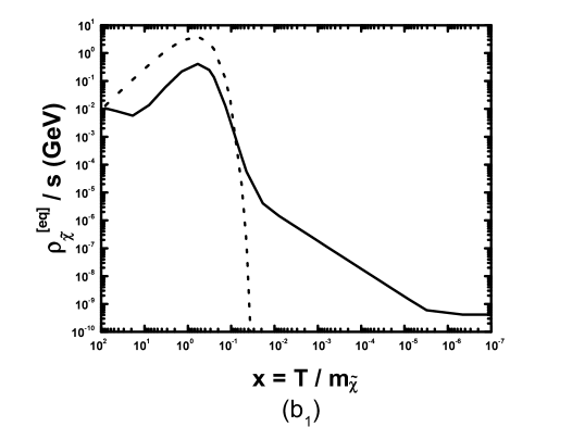
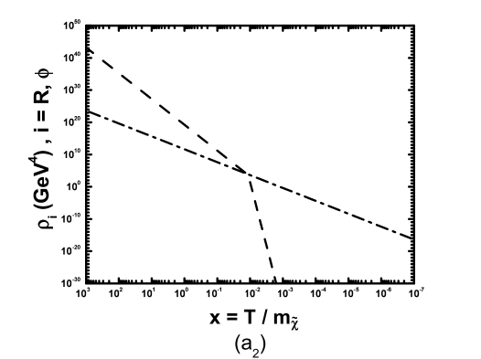
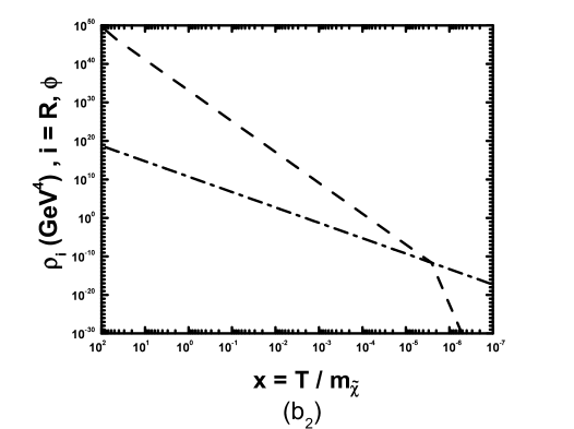
Figure 1: ${\sf(a_{1},b_{1})}$ The quantity $\rho^{[\rm eq]}_{\tilde{\chi}}/s$ (solid [dotted] line) and ${\sf(a_{2},b_{2})}$ the $\phi$ [radiation] energy densities $\rho_{\phi[{{}_{\rm R}}]}$ (dashed [dot dashed] line) versus $x=T/m_{\tilde{\chi}}$. We take $m_{\phi}=10^{6}~{}{\rm GeV},m_{\tilde{\chi}}=350~{}{\rm GeV},\langle\sigma v\rangle=10^{-10}~{}{\rm GeV}^{-2}$ and $T_{\rm RH}=5~{}{\rm GeV},~{}N_{\tilde{\chi}}=1.4\times 10^{-7}$ ${\sf(a_{1},a_{2})}$ for EP or $T_{\rm RH}=0.001~{}{\rm GeV},~{}N_{\tilde{\chi}}=1.2\times 10^{-3}$ ${\sf(b_{1},b_{2})}$ for non-EP. In both cases, we extract $\Omega_{\tilde{\chi}}h^{2}=0.115$.

$\bullet$ In both cases, $T_{\rm max}=x_{\rm max}m_{\tilde{\chi}}>T_{\rm rh}=x_{\rm rh}m_{\tilde{\chi}}$, with $x_{\rm rh}$ being derived by solving Eq. (9) and corresponding to $(R/R_{\rm I})_{\rm rh}\gg(R/R_{\rm I})_{0}$ (see Fig. 1). Our definition in Eq. (10) allows us to approach quite successfully $x_{\rm rh}$ by $x_{{}_{\rm RH}}$ (in contrast with Ref. [19]). Our $T_{\rm max}\sim m^{1/4}_{\phi}M^{1/4}_{\rm P}T^{1/2}_{\rm RH}$, in accord with Ref. [19], turns out to be larger by about one order of magnitude than this, estimated in Ref. [24].

$\bullet$ In both cases, $T_{\rm max}>m_{\tilde{\chi}}>T_{\rm RH}/x_{{}_{\rm F}(\ast)}$. This means that $\tilde{\chi}$ is first relativistic and then becomes non-relativistic, and so, its characterization as cold relic is self-consistent.

$\bullet$ In Fig 2-${\sf(a~{}[b])}$, we have $T_{\rm max}\simeq[<]m_{\phi}$. So, our perturbative approach to the $\phi$ decay is well defined [24] and possible effects of plasma masses are certainly negligible [40].

Let us finally note that hard-hard and hard-soft contributions to $\Omega_{\tilde{\chi}}h^{2}$ [24] are not included in our approach. For the ranges of Eqs (53) and (54), the hard-hard contributions are certainly negligible, whereas the hard-soft are mostly sub-dominant, since $m_{\phi}\gg m_{\tilde{\chi}}$.

4.2 NUMERICAL VERSUS SEMI-ANALYTICAL RESULTS

FIG.	RANGES OF $x$-AXIS PARAMETERS		$\tilde{\chi}$-PRO-	$\delta_{\rm RH}$
	$m_{\tilde{\chi}}=200~{}{\rm GeV}$	$m_{\tilde{\chi}}=500~{}{\rm GeV}$	DUCTION
2-${\sf(a_{1})}$	$(0.001-0.07)~{}{\rm GeV}$	$(0.001-0.12)~{}{\rm GeV}$	non-EP	$0.8$
	$(0.07-2.5)~{}{\rm GeV}$	$(0.12-4)~{}{\rm GeV}$	EP	$1.1$
2-${\sf(b_{1})}$	$(10^{3}-10^{7})~{}{\rm GeV}$		non-EP	$0.8$
2-${\sf(c_{1})}$	$10^{-7}-10^{-3}$		non-EP	$0.8$
2-${\sf(a_{2})}$	$(0.001-0.015)~{}{\rm GeV}$	$(0.0015-0.0052)~{}{\rm GeV}$	EP	$0.75$
	$(0.4-100)~{}{\rm GeV}$	$(1-100)~{}{\rm GeV}$	EP	$0.8$
2-${\sf(b_{2})}$	$(10^{3}-10^{9})~{}{\rm GeV}$		EP	$0.85$
	$(10^{9}-10^{13})~{}{\rm GeV}$		EP	$1.1$
2-${\sf(c_{2})}$	$10^{-10}-10^{-6}$		EP	$0.85$
	$10^{-6}-1$		EP	$1.1$

Table 1: The type of $\tilde{\chi}$-production and the chosen $\delta_{\rm RH}$’s for various ranges of the $x$-axis para-meters and $m_{\tilde{\chi}}$’s in Fig. 2.

The validity of our semi-analytical approach can be tested by comparing its results for $\Omega_{\tilde{\chi}}h^{2}$ with those obtained by the numerical solution of Eqs (3)-(5). In addition, useful conclusions can be inferred for the behavior of $\Omega_{\tilde{\chi}}h^{2}$ as a function of our free parameters and the regions where each ${\tilde{\chi}}$-production mechanism can be activated.

Our results are presented in Fig. 2. The solid lines are drawn from our numerical code, whereas crosses are obtained by employing (with $\delta_{\rm F}=1$) Eq. (31 [43]) for [non] EP and solving numerically Eq. (49) with a convenient $\delta_{\rm RH}$ (comments on the validity of Eq. (52) are given, too). The type of ${\tilde{\chi}}$-production and the chosen $\delta_{\rm RH}$’s for the parameters used in Fig. 2 are arranged in Table 2.

The light [normal] grey lines and crosses correspond to $m_{\tilde{\chi}}=200~{}[500]~{}{\rm GeV}$. In Fig. 2-${\sf(a_{1},b_{1},c_{1}~{}[a_{2},b_{2},c_{2}])}$, we fixed $\langle\sigma v\rangle=10^{-12}~{}[10^{-8}]~{}{\rm GeV^{-2}}$. We design $\Omega_{\tilde{\chi}}h^{2}$ versus:

$\bullet$ $T_{\rm RH}$, in Fig. 2-${\sf(a_{1}\ [a_{2}])}$ for $N_{\tilde{\chi}}=10^{-6}~{}[10^{-3}]$ and $m_{\phi}=10^{6}~{}{\rm GeV}$. Taking into account Table 2, also, we deduce that non-EP is accommodated for lower $\langle\sigma v\rangle$ and $T_{\rm RH}$ and higher $m_{\tilde{\chi}}$, since in these cases, $Y_{n}~{}[Y_{N}]$ in Eq. (32 [33]) decreases, facilitating the satisfaction of Eq. (35) for non-EP. The consideration of $N_{\tilde{\chi}}$ allows us to produce acceptable results for $\Omega_{\tilde{\chi}}h^{2}$ even for non-EP, in contrast with Ref. [20], where $N_{\tilde{\chi}}=0$. When $\Omega_{\tilde{\chi}}h^{2}$ increases with $T_{\rm RH}$, Eq. (52b) works well. However, for larger $\langle\sigma v\rangle$ and/or $T_{\rm RH}$, $\Omega_{\tilde{\chi}}h^{2}$ decreases, when $T_{\rm RH}$ increases (Fig. 2-${\sf(a_{2})}$). None of Eqs (52) works in this regime and so, the numerical solution of Eq. (49) is indispensable. For $m_{\tilde{\chi}}=200~{}[500]~{}{\rm GeV},\langle\sigma v\rangle=10^{-8}~{}{\rm GeV^{-2}}$ and $T_{\rm RH}>8.8~{}[22.5]~{}{\rm GeV}$, ${\tilde{\chi}}$ de-couples for $x<x_{{}_{\rm RH}}$ (see sec. 3.4).

$\bullet$ $m_{\phi}$, in Fig. 2-${\sf(b_{1}~{}[b_{2}])}$ for $N_{\tilde{\chi}}=10^{-6}~{}[10^{-3}]$ and $T_{\rm RH}=0.05~{}[5]~{}{\rm GeV}$. In both cases, $\Omega_{\tilde{\chi}}h^{2}$ decreases as $m_{\phi}$ increases. Eq. (52${\sf b~{}[a]}$) gives reliable results for $m_{\phi}>10^{9}$ and $m_{\tilde{\chi}}=500~{}[200]~{}{\rm GeV}$ in Fig. 2-${\sf(b_{2})}$ and for the parameters of Fig. 2-${\sf(b_{1})}$.

$\bullet$ $N_{\tilde{\chi}}$, in Fig. 2-${\sf(c_{1}~{}[c_{2}])}$ for $T_{\rm RH}=0.05~{}[5]~{}{\rm GeV}$ and $m_{\phi}=10^{6}~{}{\rm GeV}$. We observe that $\Omega_{\tilde{\chi}}h^{2}$ increases with $N_{\tilde{\chi}}$. Eq. (52${\sf b~{}[a]}$) gives reliable results for $N_{\tilde{\chi}}<10^{-6}$ and $m_{\tilde{\chi}}=500~{}[200]~{}{\rm GeV}$ in Fig. 2-${\sf(c_{2})}$ and for the parameters of Fig. 2-${\sf(c_{1})}$.

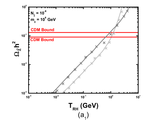
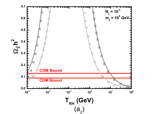
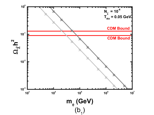
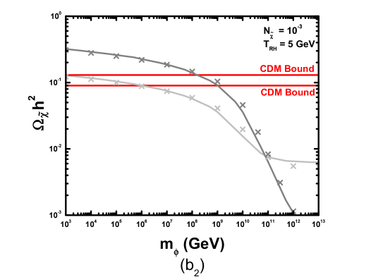
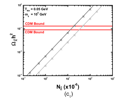
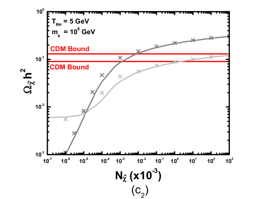
Figure 2: $\Omega_{\tilde{\chi}}h^{2}$ versus $T_{\rm RH}~{}{\sf(a_{1},a_{2})}$, $m_{\phi}~{}{\sf(b_{1},b_{2})}$ and $N_{\tilde{\chi}}~{}{\sf(c_{1},c_{2})}$ for fixed (indicated in the graphs) $N_{\tilde{\chi}}$ and $m_{\phi}$, $N_{\tilde{\chi}}$ and $T_{\rm RH}$, $T_{\rm RH}$ and $m_{\phi}$ correspondingly. We take $m_{\tilde{\chi}}=200~{}[500]~{}{\rm GeV}$ (light [normal] grey lines and crosses) and $\langle\sigma v\rangle=10^{-12}~{}[10^{-8}]~{}{\rm GeV^{-2}}~{}{\sf(a_{1},b_{1},c_{1}~{}[a_{2},b_{2},c_{2}])}$. The solid lines [crosses] are obtained by our numerical code [semi-analytical expressions].

Comparing Fig. 2-${\sf(b_{1}~{}[b_{2}])}$ and Fig. 2-${\sf(c_{1}~{}[c_{2}])}$, it can be induced that $\Omega_{\tilde{\chi}}h^{2}$ remains invariant for constant $N_{\tilde{\chi}}m^{-1}_{\phi}$. This can be understood by the observation that $y_{{}_{N}}$ in Eq. (30) is proportional to this quantity. The adjustment of $\delta_{\rm RH}$ turns out to be crucial, in order for the results from the semi-analytical treatment to approach the numerical ones. However, this kind of uncertainties is unavoidable to such approximations (see Ref. [19]). Note that the accuracy of our approximations increases as $N_{\tilde{\chi}}m^{-1}_{\phi}$ is reduced.

4.3 ALLOWED REGIONS

Requiring $\Omega_{\tilde{\chi}}h^{2}$ to be confined in the cosmologically allowed range of Eq. (2), one can restrict the free parameters. The data is derived exclusively by the numerical program.

Our results are presented in Fig. 3. The light [normal] grey regions are constructed for $m_{\tilde{\chi}}=200~{}[500]~{}{\rm GeV}$. In Fig. 3-${\sf(a_{1},b_{1},c_{1}~{}[a_{2},b_{2},c_{2}])}$, we fixed $\langle\sigma v\rangle=10^{-12}~{}[10^{-8}]~{}{\rm GeV^{-2}}$. We display the allowed regions on the:

$\bullet$ $N_{\tilde{\chi}}-T_{\rm RH}$ plane, in Fig. 3-${\sf(a_{1},a_{2})}$ for $m_{\phi}=10^{6}~{}{\rm GeV}$. Since $\Omega_{\tilde{\chi}}h^{2}$ increases with $T_{\rm RH}$ for low $\langle\sigma v\rangle$ ’s, the increase of $T_{\rm RH}$ requires diminution of $N_{\tilde{\chi}}$ in Fig. 3-${\sf(a_{1})}$. On the contrary, in Fig. 3-${\sf(a_{2})}$, when decrease of $\Omega_{\tilde{\chi}}h^{2}$ is achieved with increase of $T_{\rm RH}$ for $T_{\rm RH}\gtrsim 2~{}{\rm GeV}$, augmentation of $N_{\tilde{\chi}}$ is needed for increasing $T_{\rm RH}$.

$\bullet$ $N_{\tilde{\chi}}-m_{\phi}$ plane, in Fig. 3-${\sf(b_{1}~{}[b_{2}])}$ for $T_{\rm RH}=0.05~{}[5]~{}{\rm GeV}$. Since in both cases, $\Omega_{\tilde{\chi}}h^{2}$ in[de]-creases as $N_{\tilde{\chi}}~{}[m_{\phi}]$ increases, increase of $N_{\tilde{\chi}}$ entails increase of $m_{\phi}$.

$\bullet$ $T_{\rm RH}-m_{\phi}$ plane, in Fig. 3-${\sf(c_{1}~{}[c_{2}])}$ for $N_{\tilde{\chi}}=10^{-6}~{}[10^{-3}]$. Since for $T_{\rm RH}\lesssim 2~{}{\rm GeV}$, $\Omega_{\tilde{\chi}}h^{2}$ increases with $T_{\rm RH}$ (see Fig. 2-${\sf(a_{1},a_{2})}$) $m_{\phi}$ is to increase with $T_{\rm RH}$, as in Fig. 3-${\sf(c_{1})}$. Similar region exists, also, for the parameters used in Fig. 3-${\sf(c_{2})}$. However, for the sake of illustration, in Fig. 3-${\sf(c_{2})}$ we concentrated on the regions with $T_{\rm RH}\gtrsim 2~{}{\rm GeV}$. In these, increase of $m_{\phi}$ is dictated with decrease of $T_{\rm RH}$, since the latter causes increase of $\Omega_{\tilde{\chi}}h^{2}$, as shown in Fig. 2-${\sf(a_{2})}$. The upper [lower] bounds of the allowed areas are derived from the saturation of Eq. (2${\sf a~{}[b]}$) (inversely to all other cases).

Note, finally, that in the standard paradigm, $\Omega_{\tilde{\chi}}h^{2}$ is $(m_{\phi},N_{\tilde{\chi}},T_{\rm RH})$-independent and turns out to be almost $143-146~{}[0.022-0.023]$ for $\langle\sigma v\rangle=10^{-12}~{}[10^{-8}]~{}{\rm GeV^{-2}}$ and $m_{\rm LSP}$ varying within the range of Eq. (54a). This is easily extracted by solving Eq. (5) with $N_{\tilde{\chi}}=0$ and only a RD background in Eq. (6) with $g_{\rho\ast}$ fixed at $x_{{}_{\rm F}}m_{\tilde{\chi}}$ with $17\lesssim x^{-1}_{{}_{\rm F}}\lesssim 26$. We checked that this result agrees with this obtained by solving Eq. (76) of Ref. [12].

5 CONCLUSIONS-OPEN ISSUES

We considered a deviation from the standard cosmological situation according to which the CDM candidate, $\tilde{\chi}$ decouples from the plasma (i) during the RD era (i.e. after reheating) (ii) being in equilibrium (iii) produced through thermal scatterings. On the contrary, we assumed that $\tilde{\chi}$ decoupling occurs (i^′) during a decaying-massive-particle, $\phi$, dominated era (and mainly before reheating) (ii^′) being or not in chemical equilibrium with the thermal bath (iii^′) produced by thermal scatterings and directly from the $\phi$ decay.

We solved the problem (i) numerically, integrating the relevant system of the differential equations (ii) semi-analytically, producing approximate relations for the cosmological evolution before reheating and solving the properly re-formulated Boltzmann equations.

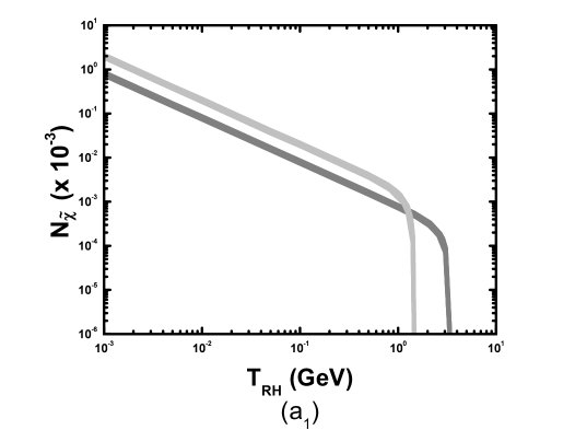
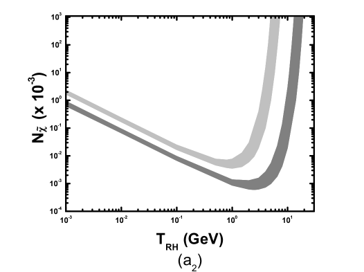
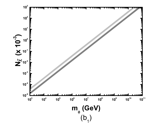
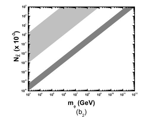
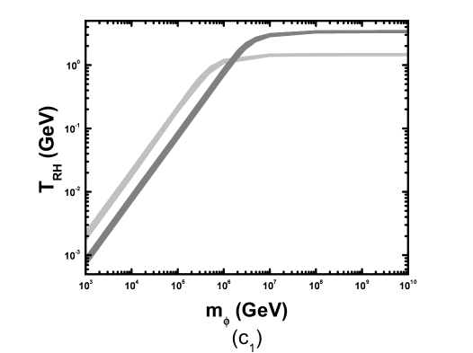
Figure 3: Regions allowed by Eq. (2) on the $T_{\rm RH}-N_{\tilde{\chi}}$ plane ${\sf(a_{1},a_{2})}$ for $m_{\phi}=10^{6}~{}{\rm GeV}$, $m_{\phi}-N_{\tilde{\chi}}$ plane ${\sf(b_{1}~{}[b_{2}])}$ for $T_{\rm RH}=0.05~{}[5]~{}{\rm GeV}$ and $m_{\phi}-T_{\rm RH}$ plane ${\sf(c_{1}~{}[c_{2}])}$ for $N_{\tilde{\chi}}=10^{-6[3]}$. We take $m_{\tilde{\chi}}=200~{}[500]~{}{\rm GeV}$ (light grey [normal grey] areas) and $\langle\sigma v\rangle=10^{-12}~{}[10^{-8}]~{}{\rm GeV^{-2}}~{}{\sf(a_{1},b_{1},c_{1}~{}[a_{2},b_{2},c_{2}])}$.

The second way facilitates the understanding of the problem and gives, in most cases, sufficiently accurate results, provided a suitable $\delta_{\rm RH}$ is chosen. The variation of $\Omega_{\tilde{\chi}}h^{2}$ w.r.t our free parameters $(m_{\phi},N_{\tilde{\chi}},T_{\rm RH})$ was investigated and regions consistent with the present CDM bounds are constructed, using $m_{\tilde{\chi}}$’s and $\langle\sigma v\rangle$’s commonly allowed in SUSY models.

These scenaria obviously let intact the SUSY parameter space but require rather low $T_{\rm RH}$. This can be accommodated in AMSBM [26], in models with intermediate scale unification [32] and within the context of $q$-balls decay [28]. Also, low $T_{\rm RH}$ naturally arises in models of thermal inflation [41] which, as a bonus, may overcome the problem of unwanted relics (e.g., gravitino, moduli). Finally, restrictions on $T_{\rm RH}$ arising from baryogenesis and neutrino cosmology have been, also, studied in Refs [42, 43].

Our formalism can be easily extended to include coannihilations and pole effects. Therefore, it can become applicable for the calculation of $\Omega_{\tilde{\chi}}h^{2}$ in the context of specific SUSY models. Also, these scenaria can assist us to the reduction of $\Omega_{\tilde{\chi}}h^{2}$ in cases, where it turns out to be even more enhanced than in the standard scenario, as in the presence of Quintessence [44]. Similar analysis of the $\tilde{\chi}$-decoupling during the extra dimensional cosmological evolution [45] may be also, possible.