Testing Non–commutative QED $\gamma\gamma\gamma$ and $\gamma\gamma\gamma\gamma$ Couplings at LHC

Abstract

In this work, we investigate the sensitivity of the process $p+p\to q+q\to j+j+\gamma+\gamma$ at LHC for the photonic 3- and 4- point functions that appear in non–commutative QED. We show that this process serves to study the behavior of the space-space as well as of the space-time non–commutativity. We also show that this process can probe the non–commutative scale $\Lambda$ in the range of few TeV s.

I Introduction

The central idea behind non–commutative space-time (NCST) is that there must be a regime of energy where space-time loses its condition of continuum and passes to obey the relation $[\hat{x}_{\mu},\hat{x}_{\nu}]=i\frac{C_{\mu\nu}}{\Lambda^{2}}$ snyder , where $C_{\mu\nu}$ is a real antisymmetric constant matrix. In other words, there must be a very microscopic region of space-time, or very high energy, where our common understanding of space-time is not applicable anymore.

When people began to develop such idea, the scale of energy $\Lambda$ where non–commutativity was expected to manifest was around the Planck scale $M_{P\ell}$ connes ; s-w . This scale of energy is quite out of the present phenomenological reach. However, inspired by this recent idea of extra dimensions extradim , which suggest the fundamental Planck scale can be around few TeV s, people brought $\Lambda$ down to TeV scale rizzo . This leaves the idea of NCST phenomenologically attainable. In this regard, it turn out to be interesting reformulate the phenomenological models in the basis of the NCST.

Unfortunately, the implementation of NCST is still a challenge for model building and presently the only consensual phenomenological model is non–commutative QED (NCQED) rizzo ; QEDphen ; mathews ; review . The phenomenology of NCQED has been intensively investigated  rizzo ; QEDphen ; mathews ; review . What has particularly called the people attention in NCQED is the photonic 3- and 4- point functions. The processes where such couplings appears are the Compton scattering, pair annihilation process, $e^{+}e^{-}\rightarrow\gamma\gamma$, and the $\gamma\gamma\rightarrow\gamma\gamma$.

However, none process involving quarks was investigate yet. The reason is that in NCQED, the covariant derivatives can only be constructed for fermionic fields of charges $0$ and $\pm 1$. Therefore, the non–commutative photon-quark-quark interaction cannot be described by the model. In order to solve this problem, people began to implement the NCST effects into the Standard Model of particles. Two proposals for Non–commutative Standard Model (NCSM) can be found in the literature, one is based on the $U_{\star}(3)\times U_{\star}(2)\times U_{\star}(1)$ gauge group ncsm1 while the other is based on the standard gauge group $SU(3)_{C}\times SU(2)_{L}\times U(1)_{Y}$, making use of the Seiberg-Witten maps ncsm2 . Some phenomenology of these models are found in Refs. ncsmphen . However, no agreement has been reached yet regarding a phenomenological NCSM.

Therefore, our main goal in this work is to study the potential of the LHC to only probe NCQED, particularly the photonic 3- and 4- point functions $\gamma\gamma\gamma$ and $\gamma\gamma\gamma\gamma$, through the process $p+p\to q+q\to j+j+\gamma+\gamma$. In order to do so, the only assumption we took is that possible non–commutative quark-quark-photon interaction generates negligible effects, allowing us to consider only the the standard model quark-quark-photon interaction and NCQED in our analysis.

This work is organized as follow. In Sec. (II) we present the photonic 3- and 4- point functions in NCQED. After in Sec. (III) we discuss the NCQED signal and the SM background. In Sec. (IV), we finish with our conclusions.

II Photonic 3- and 4- point functions in NCQED

One manner of settling non–commutative coordinates in the context of field theory is through the Moyal product, or the $\star$ product, whose expansion is connes

$$A(x)\star B(x)\equiv[e^{(i/2)\theta_{\mu\nu}\partial_{\zeta\mu}\partial_{\eta\nu}}A(x+\zeta)B(x+\eta)]_{\zeta=\eta=0}.$$ (1)

With this product, we procedure in the following way. We first formulate the Lagrangian in terms of $\star$ product and then change the $\star$ product by the expansion in (1) in order to leave the Lagrangian in terms of ordinary product.

In gauge theories first thing to do is to express the gauge transformation in terms of $\star$ products

$$A_{\mu}\rightarrow U\star A_{\mu}\star U^{-1}+\frac{i}{g}U\star\partial_{\mu}U^{-1}.$$ (2)

In the particular case of NCQED, where $U(x)=exp\star(ig\alpha(x))$, we have

$$A_{\mu}\rightarrow A_{\mu}+\partial_{\mu}\alpha-ig(A_{\mu}\star\alpha-\alpha\star A_{\mu}).$$ (3)

In order to the action of the NCQED preserves the gauge invariance, the tensor $F^{*}_{\mu\nu}$ must present the form

$$F^{*}_{\mu\nu}=\partial_{\mu}A_{\nu}-\partial_{\nu}A_{\mu}-ig[A_{\mu},A_{\nu}]_{\star}=F_{\mu\nu}-ig(A_{\mu}\star A_{\nu}-A_{\nu}\star A_{\mu}).$$ (4)

With these expansions, the photonic part of the NCQED presents the following Lagrangian

$${\cal L}= -\frac{1}{4}F^{\mu\nu}F_{\mu\nu}-2e\sin(\frac{p_{1}Cp_{2}}{2\Lambda^{2}})(\partial_{\mu}A_{\nu}-\partial_{\nu}A_{\mu})A^{\mu}A^{\nu}$$ (5)

$$-4e^{2}\sin^{2}(\frac{p_{1}Cp_{2}}{2\Lambda^{2}})A^{4},$$

where $p_{1}Cp_{2}=p_{1}^{\mu}p_{2}^{\nu}C_{\mu\nu}$ and with $F_{\mu\nu}=\partial_{\mu}A_{\nu}-\partial_{\nu}A_{\mu}$ being the standard electromagnetic tensor. The Feynman rules for the vertices $\gamma\gamma\gamma$ and $\gamma\gamma\gamma\gamma$ are given by rizzo ,

$$\gamma_{\mu}(p_{1})\gamma_{\nu}(p_{2})\gamma_{\rho}(p_{3})\; : \;2g\sin(\frac{p_{1}Cp_{2}}{2\Lambda^{2}})[(p_{1}-p_{2})^{\rho}g^{\mu\nu}+(p_{2}-p_{3})^{\mu}g^{\nu\rho}+(p_{3}-p_{1})^{\nu}g^{\mu\rho}]\;;$$

$$\gamma_{\mu}(p_{1})\gamma_{\nu}(p_{2})\gamma_{\rho}(p_{3})\gamma_{\sigma}(p_{4})\; : \;4ig^{2}[(g^{\mu\sigma}g^{\nu\rho}-g^{\mu\rho}g^{\nu\sigma})\sin(\frac{p_{1}Cp_{2}}{2\Lambda^{2}})\sin(\frac{p_{3}Cp_{4}}{2\Lambda^{2}})$$

$$+(g^{\mu\rho}g^{\nu\sigma}-g^{\mu\nu}g^{\rho\sigma})\sin(\frac{p_{3}Cp_{1}}{2\Lambda^{2}})\sin(\frac{p_{2}Cp_{4}}{2\Lambda^{2}})$$

$$+g^{\mu\nu}g^{\rho\sigma}-g^{\mu\sigma}g^{\nu\rho}()\sin(\frac{p_{1}Cp_{4}}{2\Lambda^{2}})\sin(\frac{p_{2}Cp_{3}}{2\Lambda^{2}})]\;,$$

where all the momenta are out-going.

The parametrization suggested by Hewett-Petriello-Rizzo rizzo for the antisymmetric matrix $C$ is

$$C_{\mu\nu}=\left(\begin{array}[]{cccc}0&\sin\alpha\cos\beta&\sin\alpha\sin\beta&\cos\alpha\\ -\sin\alpha\cos\beta&0&\cos\gamma&-\sin\gamma\sin\beta\\ -\sin\alpha\sin\beta&-\cos\gamma&0&-\sin\gamma\cos\beta\\ -\cos\alpha&\sin\gamma\sin\beta&\sin\gamma\cos\beta&0\end{array}\right),$$ (11)

where the three angles used to parametrize $C_{\mu\nu}$ are related with the direction of the background E and B-fields. In this parametrization, the angle $\beta$ define the origin of the $\phi$ axis rizzo . The common procedure here is to fix $\phi$ by settling $\beta=\pi/2$. Therefore, the antisymmetric matrix get parametrized by two angles: the angle $\alpha$ related to the space-time non–commutativity, and the angle $\gamma$ related to the space-space non–commutativity.

In order to test the NCQED vertexes given by equations (II), we perform a detailed analysis of the production via weak boson fusion(WBF) of photon pairs accompanied by jets, i.e.,

$$p+p\to q+q\to j+j+\gamma+\gamma\;.$$ (12)

Beyond the expected SM Feynman diagrams, reaction (12) receives contributions from NCQED photonic 3- and 4- point functions, shown in Fig. 1.

Figure 1: NCQED photonic 3- and 4- point functions contributions for the reaction (12).

The advantage of WBF, where the scattered final-state quarks receive significant transverse momentum and are observed in the detector as far-forward/backward jets, is the strong reduction of QCD backgrounds due to the kinematical configuration of the colored part of the event.

III Signals and backgrounds

In this section we study the reaction (12) at the LHC. We evaluated numerically the helicity amplitudes of all the SM subprocesses leading to the $jj\gamma\gamma$ final state where $j$ can be either a gluon, a quark or an anti-quark in our partonic Monte Carlo. The SM amplitudes were generated using Madgraph mad in the framework of Helas helas routines. The NCQED interactions arising from the Lagrangian (5) were implemented as subroutines and were included accordingly. We consistently took into account the effect of all interferences between the NCQED and the SM amplitudes, and considered a center–of–mass energy of 14 TeV and an integrated luminosity of 100 fb^-1 for LHC.

The process (12) receives contributions from the NCQED $\gamma\gamma\gamma$ and $\gamma\gamma\gamma\gamma$ vertices. In order to reduce the enormous QCD background we must exploit the characteristics of the WBF reactions. The main feature of WBF processes is a pair of very far forward/backward tagging jets with significant transverse momentum and large invariant mass between them. Therefore, we required that the jets should comply with

$$p_{T}^{j_{1(2)}}>40~{}(20)\;\text{GeV}\;\;\;\;\hbox{,}\;\;\;\;|\eta_{j_{(1,2)}}|<5.0\;,$$

$$|\eta_{j_{1}}-\eta_{j_{2}}|>4.4\;\;\;\;\hbox{,}\;\;\;\;\;\;\eta_{j_{1}}\cdot\eta_{j_{2}}<0\;\;\;\;\hbox{and}$$ (13)

$$\Delta R_{jj}>0.7\;.$$

Furthermore, the photons are central, typically being between the tagging jets. So, we require that the photons satisfy

$$E_{T}^{\gamma_{(1,2)}}>25\;\text{GeV}\;\;\;\;\hbox{,}\;\;\;\;|\eta_{\gamma_{(1,2)}}|<2.5\;,$$

$$\text{min}\{\eta_{j_{1}},\eta_{j_{2}}\}+0.7<\eta_{\gamma_{(1,2)}}<\text{max}\{\eta_{j_{1}},\eta_{j_{2}}\}-0.7\;,$$ (14)

$$\Delta R_{j\gamma}>0.7\;\;\;\;\hbox{and}\;\;\;\;\Delta R_{\gamma\gamma}>0.4\;.$$

Several kinematic distributions were evaluated in order to reduce the SM background with minimum impact over the NCQED signal. Better results were observed in three distributions: the azimuthal angle distribution of the most energetic final photon ($\Phi_{\gamma 1}$), the azimuthal angle distribution of the least energetic final photon ($\Phi_{\gamma 2}$), and the invariant mass distribution of the $\gamma\gamma$ pair ($m_{\gamma\gamma}$), presented in Fig. 2. It is interesting to notice that the presence of an NCQED signal changes the behavior of the azimuthal angle distribution of a final photon, while other known examples of new physics can not produce similar effect. However, an impressive reduction of the SM background with small effect over the NCQED signal can be achieved by a cut in the invariant mass distribution of the $\gamma\gamma$ pairs. As illustrated in Fig. 2, the invariant mass distribution for the SM background contribution is a decreasing function of the $\gamma\gamma$ invariant mass while the NCQED contribution first increases with the $\gamma\gamma$ invariant mass reaching its maximum value at $m_{\gamma\gamma}\sim 850$ GeV and then decreases. Consequently, in order to enhance the WBF signal for the NCQED $\gamma\gamma\gamma$ and $\gamma\gamma\gamma\gamma$ couplings we imposed the following additional cut in the diphoton invariant mass spectrum

$$400\text{ GeV }\leq m_{\gamma\gamma}\leq 2500\text{ GeV.}$$ (15)

The results presented in Fig. 2 were obtained using $\sqrt{\hat{s}}$ as the factorization scale in the parton distribution functions, and the renormalization scale ($\mu_{R}$) used in the evaluation of the QCD coupling constant [$\alpha_{S}(\mu_{R})$] was defined such that $\alpha_{s}^{2}(\mu_{R})=\alpha_{s}(p_{T}^{j1})\alpha_{s}(p_{T}^{j2})$, where $p_{T}^{j1}$ and $p_{T}^{j2}$ are the transverse momentum of the tagging jets.

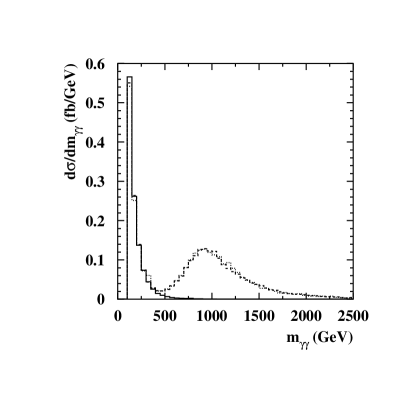
Figure 2: Azimuthal angle distribution of the most energetic final photon ($\Phi_{\gamma 1}$), azimuthal angle distribution of the least energetic final photon ($\Phi_{\gamma 2}$), and invariant mass distribution of the $\gamma\gamma$ pair ($m_{\gamma\gamma}$) for the reaction $pp\to\gamma\gamma jj$. The full line represents the SM distribution. The NCQED contribution was obtained for $\Lambda=250$ GeV, and the angles $\alpha,\beta$ and $\gamma$ equal to $\pi/2$. The dashed (dotted) line represents the space-space (space-time) non–commutativity case, discussed in the text.

The evaluation of the SM background ($\sigma_{\text{sm}}$) deserves some special care since it has a large contribution from QCD subprocesses whose size depends on the choice of the renormalization scale used in the evaluation of the QCD coupling constant, $\alpha_{s}(\mu_{R})$, as well as on the factorization scale $\mu_{F}$ used for the parton distribution functions. To estimate the uncertainty associated with these choices, we have reproduced the procedure used in Ref. Eboli:2003nq , computing $\sigma_{\text{sm}}$ for two sets of renormalization scales, which we label as $\mu_{R1,2}(\xi)$, and for several values of $\mu_{F}$. $\mu_{R1}(\xi)$ is defined such that $\alpha_{s}^{2}(\mu_{R1}(\xi))=\alpha_{s}(\xi p_{T}^{j1})\alpha_{s}(\xi p_{T}^{j2})$ where $p_{T}^{j1}$ and $p_{T}^{j2}$ are the transverse momentum of the tagging jets and $\xi$ is a free parameter varied between 0.1 and 10. The second choice of renormalization scale set is $\mu_{R2}(\xi)=\xi\sqrt{\hat{s}}/2$, with $\sqrt{\hat{s}}$ being the subprocess center–of-mass energy.

	$\sigma_{\text{sm}}$ (fb)
	$\mu_{R}=\mu_{R1}(\xi)$			$\mu_{R}=\mu_{R2}(\xi)$
$\xi$	$\mu_{F}=\sqrt{\hat{s}}$	$\mu_{F}=p^{T}_{\rm min}$	$\mu_{F}=\sqrt{\hat{s}}/10$	$\mu_{F}=\sqrt{\hat{s}}$	$\mu_{F}=p^{T}_{\rm min}$	$\mu_{F}=\sqrt{\hat{s}}/10$
0.10	3.2	5.3	4.1	1.3	2.2	1.7
0.25	2.2	3.6	2.8	1.1	1.9	1.4
1.00	1.4	2.4	1.9	0.91	1.5	1.2
4.00	1.1	1.8	1.4	0.78	1.3	1.0
10.0	0.94	1.6	1.2	0.71	1.2	0.96

Table 1: Results for $\sigma_{\text{sm}}$ for process Eq. (12); see text for details. All results include the effect of the cuts in Eq. (13), (III) and (15) as well as photon detection and jet-tagging efficiencies.

For now on our results will be presented assuming a 85% detection efficiency of isolated photons and jet-tagging. With this the efficiency for reconstructing the final state $j+j+\gamma+\gamma$ is $(0.85)^{4}\approx$ 52% which is included in our results . In Table 1 we list $\sigma_{\text{sm}}$ for the two sets of renormalization scales and for three values of the factorization scale $\mu_{F}=\sqrt{\hat{s}}$, $\sqrt{\hat{s}}/10$, and $p^{T}_{\rm min}$ where $p^{T}_{\rm min}={\rm min}(p_{T}^{j1},p_{T}^{j2})$. As shown in this table, we find that the predicted SM background can change by a factor of $\sim 8$ depending on the choice of the QCD scales. These results indicate that to obtain meaningful information about the presence of NCQED $\gamma\gamma\gamma$ and $\gamma\gamma\gamma\gamma$ couplings one cannot rely on the theoretical evaluation of the background. Instead one should attempt to extract the value of the SM background from data in a region of phase space where no signal is expected and then extrapolate to the signal region.

In looking for the optimum region of phase space to perform this extrapolation, one must search for kinematic distributions for which (i) the shape of the distribution is as independent as possible of the choice of QCD parameters. Furthermore, since the electroweak and QCD contributions to the SM backgrounds are of the same order, this requires that (ii) the shape of both electroweak and QCD contributions are similar. Several kinematic distributions verify condition (i), for example, the azimuthal angle separation of the two tagging jets which was proposed in Ref. Eboli:2000ze to reduce the perturbative QCD uncertainties of the SM background estimation for invisible Higgs searches at LHC. However, the totally different shape of the electroweak background in the present case, renders this distribution useless.

We found that the best sensitivity is obtained by using the $\gamma\gamma$ invariant mass. As can be seen in Fig. 2, the shape of the SM distribution is quite independent of the choice of the QCD parameters. As a consequence most of the QCD uncertainties cancel out in the ratio

$$R(\xi)=\frac{\sigma({400\text{ GeV }<m_{\gamma\gamma}<2500\text{ GeV }})}{\sigma({100\text{ GeV }<m_{\gamma\gamma}<400\text{ GeV }})}\;\;.$$ (16)

This fact is illustrated in Fig. 3 where we plot the value of the ratio $R(\xi)$ for different values of the renormalization and factorization scales. The ratio $R$ is almost invariant under changes of the renormalization scale, showing a maximum variation of the order of $\pm 6$% for a fixed value of the factorization scale. On the other hand, the uncertainty on the factorization scale leads to a maximum variation of 12% in the background estimation. We have also verified that different choices for the structure functions do not affect these results.

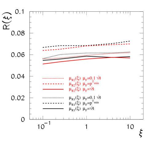
Figure 3: Ratio $R(\xi)$ defined in Eq. (16) for the process $pp\to\gamma\gamma jj$ at LHC.

Thus the strategy here proposed is simple: the experiments should measure the number of events in the $\gamma\gamma$ invariant mass window $100<m_{\gamma\gamma}<400$ GeV and extrapolate the results for higher invariant masses using perturbative QCD. According to the results described above we can conservatively assign a maximum “QCD” uncertainty (${\rm QCD}_{\rm unc}$) of $\pm$ 15% to this extrapolation.

In order to estimate the attainable sensitivity to NCQED we assume that the observed number of events is compatible with the expectations for $\mu_{R1}(\xi=1)$ and $\mu_{F}=\sqrt{\hat{s}}$, so the observed number of events in the signal region coincides with the estimated number of background events obtained from the extrapolation of the observed number of events in the region where no signal is expected; for this choice the number of expected background events is $N_{\rm sm}=\sigma_{\text{sm}}{\cal L}$ where ${\cal L}$ stands for the integrated luminosity. For an integrated luminosity of 100 fb^-1 for LHC, this corresponds to $N_{\rm back}=143$. Moreover, we have added in quadrature the statistical error and the QCD uncertainty associated with the backgrounds. Therefore, the 95% C.L. limits on $\Lambda$ can be obtained from the condition

$$N_{\rm NCQED}\,=\,{\cal L}\,\times\,\sigma_{\rm NCQED}\leq 1.95\sqrt{N_{\rm sm}+(N_{\rm sm}\times{\rm QCD}_{\rm unc})^{2}}\;,$$ (17)

where $N_{\rm NCQED}$ ($\sigma_{\rm NCQED}$) is the maximum number of events (cross section) deviation due to the NCQED contribution, so $N_{\rm observed}=N_{\rm sm}\pm N_{\rm NCQED}$. Once we have ${\cal L}=100{\rm fb}^{-1}$ and $N_{\rm back}=143$, equation (17) turns out to be

$$\sigma_{\rm NCQED}({\rm fb})\leq 0.0195\times\sqrt{143+(143\times{\rm QCD}_{\rm unc})^{2}}\;.$$ (18)

For the sake of completeness we show the results on the expected sensitivity using purely statistical errors and for two values of ${\rm QCD}_{\rm unc}$: our most conservative estimate [15 %], and a possible reduced uncertainty (7.5 %), which could be attainable provided NLO QCD calculations are available. Therefore the NCQED deviation should not be greater than the values presented in Table 2.

${\rm QCD}_{\rm unc}$	$\sigma_{\rm NCQED}({\rm fb})$	$N_{\rm NCQED}$
0	0.23	23
7.5%	0.31	31
15%	0.48	48

Table 2: 95% C.L. maximum cross section and number of events deviation due to the NCQED contribution.

Once we have fixed $\phi$ by settling $\beta=\pi/2$ in equation (11), the antisymmetric matrix get parametrized by two angles: the angle $\alpha$ related to the space-time non–commutativity, and the angle $\gamma$ related to the space-space non–commutativity. Therefore, in order to perform our analysis we consider two cases:

• (i) the space-space non–commutativity, where the elements $C_{0i}$ ($i=1,2,3$) in equation (11) are assumed to be $0$, and the angle $\gamma$ are assumed to be either $0$, $\pi/4$ or $\pi/2$;

• (ii) the space-time non–commutativity, where the elements $C_{ij}$ ($i,j=1,2,3$) in equation (11) are assumed to be $0$, and the angle $\alpha$ are assumed to be either $0$, $\pi/4$ or $\pi/2$.

Figure 4: Cross section results including the effect of the cuts in Eq. (13), (III) and (15) as well as photon detection and jet-tagging efficiencies. The solid line is the cross section including space-space NCQED effects, the dashed line is the SM cross section, and the upper (medium) [lower] dotted line represents the 95% C.L. upper limit for an QCD uncertainty of 15% (7.5%) [0].

In order to determine which case of NCQED is being observed, one can use the azimuthal angle distribution of a final photon. As illustrated in Fig. 2, the azimuthal angle distribution of either the most or the least energetic final photon for the SM background contribution is a flat function in the range $|\Phi_{\gamma}|<\frac{\pi}{2}$, while for the space-time (space-space) non–commutativity signal contribution, the distribution is increased for $|\Phi_{\gamma}|\to\frac{\pi}{2}(0)$.

The evaluation of the cross section of the reaction (12), including the effect of the cuts in Eq. (13), (III) and (15) as well as photon detection and jet-tagging efficiencies, is now done including the effect of the diagrams in Fig. (1), for the cases (i) and (ii) described above.

The results for the space-space non–commutativity, case (i), are presented in Fig. (4), for $\gamma=\pi/4$, and $\pi/2$. No limits on $\Lambda$ could be obtained for $\gamma=0$. Our analysis shows a better sensitivity for the angle $\gamma=\pi/2$, allowing us to impose a lower limit on the NCQED scale of $\Lambda\gtrsim$ 990 GeV if the QCD uncertainty discussed above is not considered. The limit changes to $\Lambda\gtrsim$ 930 (960) GeV for a QCD uncertainty of 15% (7.5%). For $\gamma=\pi/4$, the lower limit on the NCQED scale is $\Lambda\gtrsim$ 780 (850) [900] GeV for a QCD uncertainty of 15% (7.5%) [0%].

Figure 5: Cross section results including the effect of the cuts in Eq. (13), (III) and (15) as well as photon detection and jet-tagging efficiencies. The solid line is the cross section including space-time NCQED effects, the dashed line is the SM cross section, and the upper (medium) [lower] dotted line represents the 95% C.L. upper limit for an QCD uncertainty of 15% (7.5%) [0].

On the other hand, the results for the space-time non–commutativity, case (ii), are presented in Fig. (5), for $\alpha=0$, $\pi/4$, and $\pi/2$, respectively. Our analysis shows a better sensitivity for the angle $\alpha=0$, allowing us to impose a lower limit on the NCQED scale of $\Lambda\gtrsim$ 1320 GeV if the QCD uncertainty discussed above is not considered. The limit changes to $\Lambda\gtrsim$ 1290 (1230) GeV for a QCD uncertainty of 15% (7.5%). For $\alpha=\pi/4$, the lower limit on the NCQED scale is $\Lambda\gtrsim$ 1130 (1190) [1230] GeV for a QCD uncertainty of 15% (7.5%) [0%] and for $\alpha=0$, the lower limit on the NCQED scale is $\Lambda\gtrsim$ 920 (960) [990] GeV for a QCD uncertainty of 15% (7.5%) [0%].

IV Conclusions

In this work we investigated the potential for LHC to probe the photonic 3- and 4- point functions that appears in NCQED through the analysis of the process (12). Even though we assumed that the quark-quark-photon interactions make part of the SM background due to our choice of kinematical cuts, this process is sensitive for space-space as well as for space-time non–commutativity. Our main results are presented in Fig. 4 and Fig. 5 where the space-space and space-time NCQED effects are observed.

For the space-space non–commutativity, our study shows a better sensitivity for the angle $\gamma=\pi/2$, allowing us to impose a lower limit on the NCQED scale $\Lambda$ in the range 930 GeV $\leq\Lambda\leq$ 990 GeV, depending on the perturbative QCD uncertainties considered. Regarding the space-time non–commutativity, the process is more sensitive for the angle $\alpha=0$, where a lower limit on the NCQED scale $\Lambda$ in the range 1230 GeV $\leq\Lambda\leq$ 1320 GeV, depending on the perturbative QCD uncertainties considered, could be imposed.

Therefore, this work shows that LHC may be a good place to test NCQED via the study of the process (12). We have shown that LHC is able to probe both space-space and space-time non–commutativity. A better sensitivity is expected for the space-time non–commutativity, where the NCQED scale $\Lambda$ can be tested up to $\Lambda\sim 1.25$ TeV.

- (1) H. S. Snyder , Phys. Rev. D 71, 38 (1947.)
- (2) A. Connes, M. R. Douglas and A. Schwarz, J. High Energy Phys. 9802, 003 (1998).
- (3) N. Seiberg and E. Witten, J. High Energy Phys. 9909, 032 (1999).
- (4) N. Arkani-Hamed, S. Dimopoulos and G. Dvali, Phys. Lett. B 429, 263 (1998); L. Randal and R. Sundrum, Phys. Rev. Lett. 83, 3370 (1999.)
- (5) J. L. Hewett, F. J. Petriello and T. G. Rizzo, Phys. Rev. D 64, 075012 (2001).
- (6) T. Rizzo, Int. J. Mod. Phys. A 18, 2797 (2003); S. Godfrey and M. A. Doncheski, Phys. Rev. D 65, 015005 (2002); A. Anisimov, T. Banks, M. Dine, and M. Graesser, Phys. Rev. D 65, 085032 (2002); H. Grosse and Y. Liao, Phys. Rev. D 64, 115007 (2001); S-W Baek, D. K. Ghosh, X-G He, and W. Y. P. Hwang, PRD 64 056001 2001 ; S. Godfrey and M. A. Doncheski, hep-ph/0111147; N. Mahajan, hep-ph/0110148 .
- (7) P. Mathews, Phys. Rev. D 63, 075007-1 (2001).
- (8) For an excellent review of the phenomenology of NCQED see: I. Hinchliffe and N. Kersting, hep-ph/0205040.
- (9) A. Armoni, Nucl. Phys. B 593, 229 (2001); M. Chaichian, P. Presnajder, M. M. Sheikh-Jabbari, A. Tureanu, Eur. Phys. J. C 29, 413 (2003).
- (10) X. Calmet, B. Jurco, P. Schupp, J. Wess, M. Wohlgenannt, Eur. Phys. J. C 23, 363 (2002.)
- (11) W. Behr, N.G. Deshpande, G. Duplancic, P. Schupp, J. Trampetic, J. Wess, Eur. Phys. J. C 29, 441 (2003); E. O. Iltan, Phys. Rev. D 66, 034011 (2002).
- (12) T. Stelzer and W. F. Long, Comput. Phys. Commun. 81, 357 (1994).
- (13) H. Murayama, I. Watanabe, and K. Hagiwara, KEK report 91-11 (unpublished).
- (14) O. J. P. Éboli, M. C. Gonzalez-Garcia and S. M. Lietti, hep-ph/0310141.
- (15) O. J. Éboli and D. Zeppenfeld, Phys. Lett. B 495, 147 (2000).