Effective Theory of Superfluid Quark Matter

Abstract

We provide a brief introduction to the high density effective theory of QCD. As an application, we consider the instanton correction to the perturbatively generated gap in the color superconducting phase. We show that the instanton correction becomes large for $\mu\sim 1.25$ GeV in $N_{f}=2$ QCD, and for $\mu\sim 750$ MeV in $N_{f}=3$ QCD with a massive strange quark. We also study some other numerical issues related to the magnitude of the gap. We find, in particular, that a renormalization group improved gap equation does not give results that are substantially different from a gap equation with a fixed coupling.

1 Introduction

Over the last several years we have seen rapid progress in the theoretical study of very dense hadronic matter. Many new phases of strongly interacting matter, such as color superconducting quark matter and color-flavor locked matter have been predicted [1, 2, 3, 4, 5]. Reviews of these developments can be found in [6, 7, 8, 9, 10]. Exotic phases of matter at high baryon density may be realized in nature in the cores of neutron stars. In order to study this possibility quantitatively we would like to develop a systematic framework that will allow us to determine the exact nature of the phase diagram as a function of the density, temperature, the quark masses, and the lepton chemical potentials, and to compute the low energy properties of these phases. In this contribution we give a brief review of an attempt to use effective field theory methods to address this problem.

2 High Density Effective Theory

At high baryon density the relevant degrees of freedom are particle and hole excitations which move with the Fermi velocity $v$. Since the momentum $p\sim v\mu$ is large, typical soft scatterings cannot change the momentum by very much. An effective field theory of particles and holes in QCD is given by [11, 12]

$$L=\sum_{v}\psi_{v}^{\dagger}(iv\cdot D)\psi_{v}-\frac{1}{4}G^{a}_{\mu\nu}G^{a}_{\mu\nu}+\ldots,$$ (1)

where $v_{\mu}=(1,\vec{v})$. The field describes particles and holes with momenta $p=\mu\vec{v}+l$, where $l\ll\mu$. We will write $l=l_{0}+l_{\|}+l_{\perp}$ with $\vec{l}_{\|}=\vec{v}(\vec{l}\cdot\vec{v})$ and $\vec{l}_{\perp}=\vec{l}-\vec{l}_{\|}$. In order to take into account the entire Fermi surface we have to cover the Fermi surface with patches labeled by the local Fermi velocity. The number of these patches is $n_{v}\sim(\mu^{2}/\Lambda_{\perp}^{2})$ where $\Lambda_{\perp}\ll\mu$ is the cutoff on the transverse momenta $l_{\perp}$.

Higher order terms are suppressed by powers of $1/\mu$. As usual we have to consider all possible terms allowed by the symmetries of the underlying theory. At $O(1/\mu)$ we have

$$L=\sum_{v}\left\{-\frac{1}{2\mu}\psi_{v}^{\dagger}D_{\perp}^{2}\psi_{v}-g\psi_{v}^{\dagger}\frac{\sigma^{\mu\nu}G_{\mu\nu}^{\perp}}{4\mu}\psi_{v}\right\}.$$ (2)

At higher order in $1/\mu$ there is an infinite tower of operators of the form $\mu^{-n}\psi^{\dagger}_{v}D_{\perp}^{2n_{1}}(\bar{v}\cdot D)^{n_{2}}\psi_{v}$ with $\bar{v}=(1,-\vec{v})$ and $n=2n_{1}+n_{2}-1$. At $O(1/\mu^{2})$ the effective theory contains four-fermion operators [13]

$$L = \frac{1}{\mu^{2}}\sum_{v_{i}}\sum_{\Gamma,\Gamma^{\prime}}c^{\Gamma\Gamma^{\prime}}(\vec{v}_{1}\cdot\vec{v}_{2},\vec{v}_{1}\cdot\vec{v}_{3},\vec{v}_{2}\cdot\vec{v}_{3})$$ (3)

$$\mbox{}\hskip 14.22636pt\cdot\Big{(}\psi_{v_{1}}\Gamma\psi_{v_{2}}\Big{)}\Big{(}\psi^{\dagger}_{v_{3}}\Gamma^{\prime}\psi^{\dagger}_{v_{4}}\Big{)}\delta(v_{1}+v_{2}-v_{3}-v_{4}).$$

There are two types of operators that are compatible with the restriction $v_{1}+v_{2}=v_{3}+v_{4}$. The first possibility is that both the incoming and outgoing fermion momenta are back-to-back. This corresponds to the BCS interaction

$$L=\frac{1}{\mu^{2}}\sum_{v,v^{\prime}}\sum_{\Gamma,\Gamma^{\prime}}V_{l}^{\Gamma\Gamma^{\prime}}R_{l}^{\Gamma\Gamma^{\prime}}(\vec{v}\cdot\vec{v}^{\prime})\Big{(}\psi_{v}\Gamma\psi_{-v}\Big{)}\Big{(}\psi^{\dagger}_{v^{\prime}}\Gamma^{\prime}\psi^{\dagger}_{-v^{\prime}}\Big{)},$$ (4)

where $\vec{v}\cdot\vec{v}^{\prime}=\cos\theta$ is the scattering angle and $R_{l}^{\Gamma\Gamma^{\prime}}(\vec{v}\cdot\vec{v}^{\prime})$ is a set of orthogonal polynomials. The second possibility is that the final momenta are equal to the initial momenta up to a rotation around the axis defined by the sum of the incoming momenta. The relevant four-fermion operator is

$$L=\frac{1}{\mu^{2}}\sum_{v,v^{\prime},\phi}\sum_{\Gamma,\Gamma^{\prime}}F_{l}^{\Gamma\Gamma^{\prime}}(\phi)R_{l}^{\Gamma\Gamma^{\prime}}(\vec{v}\cdot\vec{v}^{\prime})\Big{(}\psi_{v}\Gamma\psi_{v^{\prime}}\Big{)}\Big{(}\psi^{\dagger}_{\tilde{v}}\Gamma^{\prime}\psi^{\dagger}_{\tilde{v}^{\prime}}\Big{)},$$ (5)

where $\tilde{v},\tilde{v}^{\prime}$ are the vectors obtained from $v,v^{\prime}$ by a rotation around $v_{tot}=v+v^{\prime}$ by the angle $\phi$.

The four-fermion operators in the effective theory can be determined by matching moments of quark-quark scattering amplitudes between QCD and the effective theory. The matching conditions involve on-shell scattering amplitudes in BCS and forward kinematics. The scattering amplitude in the effective theory contains almost collinear gluon exchanges which do not change the velocity label of the quarks as well as four-fermion operators which correspond to scattering involving different patches on the Fermi surface. There are several contributions in the microscopic theory that are absorbed into four-fermion operators in the effective theory. Examples are large angle scatterings [13] and non-perturbative instanton effects [14].

3 Power Counting

In this section we briefly discuss the power counting in the high density effective theory. We will denote the small scale by $l\ll\mu$. We first discuss the scaling properties of a generic operator. We assume that $v\cdot D$ scales as $l$, $\psi_{v}$ scales as $l^{3/2}$, $A_{\mu}$ scales as $l$, and $\vec{D}_{\perp},\bar{v}\cdot D\sim l$. Complication arise because not all loop diagrams scale as $l^{4}$. In fermion loops sums over patches and integrals over transverse momenta can combine to give integrals that are proportional to the surface area of the Fermi sphere,

$$\frac{1}{2\pi}\sum_{\vec{v}}\int\frac{d^{2}l_{\perp}}{(2\pi)^{2}}=\frac{\mu^{2}}{2\pi^{2}}\int\frac{d\Omega}{4\pi}.$$ (6)

Figure 1: Counting hard loops in the effective field theory. If all (soft) gluon lines are removed the remaining fermionic loops contain sums over the velocity index.

These loop integrals scale as $l^{2}$, not $l^{4}$. In the following we will refer to loops that scale as $l^{2}$ as “hard loops” and loops that scale as $l^{4}$ as “soft loops”. In order to take this distinction into account we define $V_{k}^{S}$ and $V_{k}^{H}$ to be the number of soft and hard vertices of scaling dimension $k$. A vertex is called soft if it contains no fermion lines. In order to determine the $l$ counting of a general diagram in the effective theory we remove all gluon lines from the graph, see Fig. 1. We denote the number of connected pieces of the remaining graph by $N_{C}$. Using Euler identities for both the initial and the reduced graph we find that the diagram scales as $l^{\delta}$ with

$$\delta=\sum_{i}\left[(k-4)V_{k}^{S}+(k-2-f_{k})V_{k}^{H}\right]+E_{Q}+4-2N_{C}.$$ (7)

Here, $f_{k}$ denotes the number of fermion fields in a hard vertex, and $E_{Q}$ is the number of external quark lines. We observe that in general the scaling dimension $\delta$ increases with the number of higher order vertices, but there are two important exceptions.

First we observe that the number of disconnected fermion loops, $N_{C}$, reduces the power $\delta$. Each disconnected loop contains at least one power of the coupling constant, $g$, for every soft vertex. As a result, fermion loop insertions in gluon $n$-point functions spoil the power counting if the gluon momenta satisfy $l\sim g\mu$. This implies that for $l<g\mu$ the high density effective theory becomes non-perturbative and fermion loops in gluon $n$-point functions have to be resummed. The generating functional for hard dense loops in gluon $n$-point functions is given by [15, 16]

$$L_{HDL}=-m^{2}\int\frac{d\Omega}{4\pi}{\rm Tr}\,G_{\mu\alpha}\frac{\hat{P}^{\alpha}\hat{P}^{\beta}}{(\hat{P}\cdot D)^{2}}G^{\mu}_{\,\beta},$$ (8)

where $m^{2}=N_{f}g^{2}\mu^{2}/(4\pi^{2})$ and the angular integral corresponds to an average over the direction of $\hat{P}_{\alpha}=(1,\hat{p})$. For momenta $l<g\mu$ we have to add $L_{HDL}$ to $L_{HDET}$. In order not to over-count diagrams we have to remove at the same time all diagrams that become disconnected if all soft gluon lines are deleted. Note that the high density effective theory is different from the standard hard dense loop approximation, because hard loops are resummed only in gluon Green functions, but not in quark Green functions or quark-gluon vertex functions.

The second observation is that the power counting for hard vertices is modified by a factor that counts the number of fermion lines in the vertex. It is easy to see that four-fermion operators without extra derivatives are leading order ($k-2-f_{k}=0$), but terms with more than four fermion fields, or extra derivatives, are suppressed. This result is familiar from the effective field theory analysis of theories with short range interactions [17, 18].

4 Color Superconductivity

In the last section we saw that hard loops lead to non-perturbative effects in the effective theory that require resummation at the scale $l\sim g\mu$. In addition to that, there are logarithmic divergences that have to be resummed at exponentially small scales $l\sim\mu\exp(-c/g)$. The most important effect of this type is the BCS instability in the quark-quark scattering amplitude. This instability leads to the formation of a gap in the single particle spectrum. We can take this effect into account in the high density effective theory by including a tree level gap term

$$L=\Delta\,R_{l}^{\Gamma}(\vec{v}\cdot\hat{\Delta})\psi_{-v}\sigma_{2}\Gamma\psi_{v}+h.c..$$ (9)

The Dirac matrix $\Gamma$ and the angular factor $R_{l}^{\Gamma}(x)$ determine the helicity and partial wave channel. The magnitude of the gap is determined variationally, by requiring the free energy to be stationary order by order in perturbation theory.

At leading order in the high density effective theory the variational principle for the gap $\Delta$ gives the Dyson-Schwinger equation

$$\Delta(p_{4})=\frac{2g^{2}}{3}\int\frac{d^{4}q}{(2\pi)^{4}}\frac{\Delta(q_{4})}{q_{4}^{2}+l_{q}^{2}+\Delta(q_{4})^{2}}v_{\mu}v_{\nu}D_{\mu\nu}(p-q),$$ (10)

where we have restricted ourselves to angular momentum zero and the color anti-symmetric $[\bar{3}]$ channel. $D_{\mu\nu}$ is the hard dense loop resummed gluon propagator. We also note that equ. (10) only contains collinear exchanges. According to the arguments give in Sect. 3 four-fermion operators are of leading order in the HDET power counting. However, even though collinear exchanges and four-fermion operators have the same power of $l$, collinear exchanges are enhanced by a logarithm of the small scale. As a consequence, we can treat four-fermion operators as a perturbation.

Sine the electric interaction is screened it is possible to absorb electric gluon exchanges into four-fermion operators. At leading order in the high density theory the gap equation is completely determined by the collinear divergence in the magnetic gluon exchange interaction. This IR divergence is independent of the helicity and angular momentum channel. We have

$$\Delta(p_{4})=\frac{g^{2}}{18\pi^{2}}\int_{0}^{\Lambda_{\|}}dq_{4}\frac{\Delta(q_{4})}{\sqrt{q_{4}^{2}+\Delta(q_{4})^{2}}}\log\left(\frac{\Lambda_{\perp}}{|p_{4}^{2}-q_{4}^{2}|^{1/2}}\right).$$ (11)

The leading logarithmic behavior is independent of the ratio of the cutoffs and we can set $\Lambda_{\|}=\Lambda_{\perp}=\Lambda$. We introduce the dimensionless variables variables $x=\log(2\Lambda/(q_{4}+\epsilon_{q}))$ and $y=\log(2\Lambda/(p_{4}+\epsilon_{p})$ where $\epsilon_{q}=(q_{4}^{2}+\Delta(q_{4}))^{1/2}$. In terms of dimensionless variables the gap equation is given by

$$\Delta(y)=\frac{g^{2}}{18\pi^{2}}\int_{0}^{x_{0}}dx\,\Delta(x)K(x,y),$$ (12)

where $x_{0}=\log(2\Lambda/\Delta_{0})$ and $K(x,y)$ is the kernel of the integral equation. At leading order we can use the approximation $K(x,y)=\min(x,y)$. We can perform an additional rescaling $x=x_{0}\bar{x}$, $y=x_{0}\bar{y}$. Since the leading order kernel is homogeneous in $x$ and $y$ we can write the gap equation as an eigenvalue equation

$$\Delta(\bar{y})=x_{0}^{2}\frac{g^{2}}{18\pi^{2}}\int_{0}^{1}d\bar{x}\,\Delta(\bar{x})K(\bar{x},\bar{y}),$$ (13)

where the gap function is subject to the boundary conditions $\Delta(0)=0$ and $\Delta^{\prime}(1)=0$. This integral equation has the solutions [19]

$$\Delta_{n}(\bar{x})=\Delta_{n,0}\sin\left(\frac{g}{3\sqrt{2}\pi}x_{0,n}\bar{x}\right),\hskip 5.69046ptx_{0,n}=(2n+1)\frac{3\pi^{2}}{\sqrt{2}g}.$$ (14)

The physical solution corresponds to $n=0$ which gives the largest gap, $\Delta_{0}=2\Lambda\exp(-3\pi^{2}/(\sqrt{2}g))$. Solutions with $n\neq 0$ have smaller gaps and are not global minima of the free energy.

5 Higher Order Corrections to the Gap

The high density effective field theory enables us to perform a systematic expansion of the kernel of the gap equation in powers of the small scale and the coupling constant. It is not so obvious, however, how to solve the gap equation for more complicated kernels, and how the perturbative expansion of the kernel is related to the expansion of the solution of the gap equation.

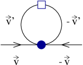
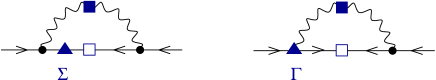
Figure 2: Higher order corrections to the gap equation in the high density effective theory. The diagrams shown in this figure correspond to four-fermion operators, fermion self-energy corrections, and vertex corrections.

For this purpose it is useful to develop a perturbative method for solving the gap equation [20, 13]. We can write the kernel of the gap equation as $K(x,y)=K_{0}(x,y)+\delta K(x,y)$, where $K_{0}(x,y)$ contains the leading IR divergence and $\delta K(x,y)$ is a perturbation. We expand both the gap function $\Delta(x)$ and the eigenvalue $x_{0}$ order by order $\delta K$,

$$\Delta(\bar{x}) = \Delta^{(0)}(\bar{x})+\Delta^{(1)}(\bar{x})+\Delta^{(2)}(\bar{x})+\ldots,$$ (15)

$$\bar{x}_{0} = \bar{x}_{0}^{(0)}+\bar{x}_{0}^{(1)}+\bar{x}_{0}^{(2)}+\ldots,$$ (16)

where we have defined $\bar{x}_{0}^{2}=g^{2}x_{0}^{2}/(18\pi^{2})$. The expansion coefficients can be found using the fact that the unperturbed solutions given in equ. (14) form an orthogonal set of eigenfunctions of $K_{0}$. The resulting expressions for $\bar{x}_{0}^{(i)}$ and $\Delta^{(i)}(\bar{x})$ are very similar to Rayleigh-Schroedinger perturbation theory. At first order we have

$$\bar{x}_{0}^{(1)} = -\frac{1}{2}\left(\bar{x}_{0}^{(0)}\right)^{2}\int_{0}^{1}d\bar{x}\int_{0}^{1}d\bar{y}\,\Delta_{0}^{(0)}(\bar{x})\delta\bar{K}(x_{0}\bar{x},x_{0}\bar{y})\Delta_{0}^{(0)}(\bar{y}),$$ (17)

$$c^{(1)}_{k} = \frac{\bar{x}_{0}^{(0)}}{1-\left(\frac{1}{2k+1}\right)^{2}}\int_{0}^{1}d\bar{x}\int_{0}^{1}d\bar{y}\,\Delta^{(0)}_{0}(\bar{x})\delta\bar{K}(x_{0}\bar{x},x_{0}\bar{y})\Delta^{(0)}_{k}(\bar{y}),$$ (18)

with $\Delta^{(1)}(x)=\sum c_{k}^{(1)}\Delta^{(0)}_{k}(x)$ and $\delta\bar{K}=g/(3\sqrt{2}\pi)\delta K$.

We can now study the role of various corrections to the kernel. The simplest contribution arises from four-fermion operators. We find

$$\delta K(x_{0}\bar{x},x_{0}\bar{y})=\log(b),\hskip 28.45274ptb=\frac{512\pi^{4}\mu}{g^{5}\Lambda}\left(\frac{2}{N_{f}}\right)^{\frac{5}{2}}.$$ (19)

This contribution does not change the shape of the gap function but it gives an $O(g)$ correction to the eigenvalue $\bar{x}_{0}$. This corresponds to a constant pre-exponential factor, $\Delta^{(1)}=b\Delta^{(0)}$. An important advantage of the effective field theory method is that this factor is manifestly independent of the choice of gauge. The gauge independence of the pre-exponential factor is related to the fact that this coefficient is determined by four-fermion operators in the effective theory, and that these operators are determined by on-shell matching conditions.

Another effect that contributes to the eigenvalue at $O(g)$ is the fermion self energy [20, 21]. A one-loop calculation in the high density effective theory gives [22, 23, 24, 25, 26]

$$\Sigma(p_{4})=\frac{g^{2}C_{F}}{12\pi^{2}}p_{4}\log\left(\frac{\Lambda}{p_{4}}\right).$$ (20)

The correction to the kernel of the gap equation is

$$\delta\bar{K}(x_{0}\bar{x},x_{0}\bar{y})=-\frac{g^{2}}{9\pi^{2}}\left(\bar{x}_{0}\bar{x}\right)K_{0}(x_{0}\bar{x},x_{0}\bar{y}),$$ (21)

and the shift in the eigenvalue is given by

$$\bar{x}^{(1)}_{0}=-\frac{1}{2}\left(\bar{x}_{0}^{(0)}\right)^{2}\langle 0|\delta\bar{K}|0\rangle=\frac{4+\pi^{2}}{8}\frac{g}{3\sqrt{2}\pi},$$ (22)

where $\langle 0|\delta\bar{K}|0\rangle$ denotes the matrix element of the kernel between unperturbed gap functions, see equ. (17). At this order in $g$, there is no contribution from the quark-gluon vertex correction. Note that the quark self energy correction makes an $O(g)$ correction to the eigenvalue, even though it is an $O(g^{2})$ correction to the kernel. This is related to the logarithmic divergence in the self energy. The perturbative expansion of $\bar{x}_{0}$ is of the form

$$\bar{x}_{0}\sim g\log(\Delta)=O(g^{0})+O(g\log(g))+O(g)+\ldots.$$ (23)

Brown et al. argued that equ. (22) completes the $O(g)$ term. At this order the spin zero gap in the 2SC phase of $N_{f}=2$ QCD is [21, 27, 13]

$$\Delta=512\pi^{4}\mu g^{-5}e^{-\frac{4+\pi^{2}}{8}}e^{-\frac{3\pi^{2}}{\sqrt{2}g}}.$$ (24)

In other spin or flavor channels the relevant four fermion operators are different and the pre-exponential factor is modified [5, 21, 28, 29]. In the CFL phase of $N_{f}=3$ QCD the gap is suppressed by a factor $(2/3)^{5/2}2^{-1/3}$.

6 Instanton Correction

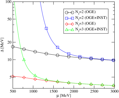
Figure 3: Instanton correction to the perturbatively generated gap in QCD with $N_{f}=2$ and $N_{f}=2+1$ flavors. We show the gap with and without instanton corrections. In the $N_{f}=2+1$ case we have used $m_{s}=150$ MeV.

In this section we shall focus on the correction to the perturbatively generated gap parameter which is due to instantons. If the density is very large instanton effects are exponentially small as compared to perturbative interactions. In this regime instantons are important for physical observables, like the mass of the $U(1)_{A}$ Goldstone mode, that receive no contribution from perturbative interactions, but they make no significant contribution to the gap. As the density is lowered instanton effects grow. In the following we will use the methods described in the last section in order to determine the scale at which instanton contributions to the gap become important.

Instantons induce a chirality changing four-fermion operator. In QCD with $N_{f}=3$ flavors and $m_{u,d}\ll m_{s}$ we have

$${L} = \int n(\rho,\mu)d\rho\,\frac{2(2\pi\rho)^{4}\rho^{3}}{4(N_{c}^{2}-1)}m_{s}\epsilon_{f_{1}f_{2}}\epsilon_{g_{1}g_{2}}\left(\frac{2N_{c}-1}{2N_{c}}(\bar{\psi}_{R,f_{1}}\psi_{L,g_{1}})(\bar{\psi}_{R,f_{2}}\psi_{L,g_{2}})\right.$$ (25)

$$\hskip 28.45274pt\mbox{}\left.-\frac{1}{8N_{c}}(\bar{\psi}_{R,f_{1}}\sigma_{\mu\nu}\psi_{L,g_{1}})(\bar{\psi}_{R,f_{2}}\sigma_{\mu\nu}\psi_{L,g_{2}})+(L\leftrightarrow R)\right),$$

where the sum over flavors runs over up and down quarks only, $f_{1,2}=g_{1,2}=(u,d)$, and the instanton size distribution $n(\rho,\mu)$ is given by

$$n(\rho,\mu) = C_{N}\ \left(\frac{8\pi^{2}}{g^{2}}\right)^{2N_{c}}\rho^{-5}\exp\left[-\frac{8\pi^{2}}{g(\rho)^{2}}\right]\exp\left[-N_{f}\rho^{2}\mu^{2}\right],$$ (28)

$$C_{N}\;=\;\frac{0.466\exp(-1.679N_{c})1.34^{N_{f}}}{(N_{c}-1)!(N_{c}-2)!}\,,$$

$$\frac{8\pi^{2}}{g^{2}(\rho)}\;=\;-b\log(\rho\Lambda),\hskip 28.45274ptb=\frac{11}{3}N_{c}-\frac{2}{3}N_{f}\,.$$

Note that equ. (25) is an effective interaction for quarks near the Fermi surface. In particular, there are no form factors that have to be included. We also observe that the integration over sizes is cut off at $\rho\sim\mu^{-1}$. As a consequence, instanton effects are of order $\exp(-8\pi^{2}/g^{2}(\mu))\sim(\Lambda_{QCD}/\mu)^{b}$. In addition to the four-fermion vertex given in equ. (25) instantons also induce a six-fermion operator. This operator has important physical effects, but it does not contribute to the gap to leading order in the effective interaction, so we will not consider it here. In QCD with $N_{f}=2$ massless flavors instantons induce a four-fermion operator which can be obtained from equ. (25) by making the replacement $m_{s}\rho\to 1$.

We can now compute the instanton correction to the kernel of the gap equation. In the three flavor case we find $\delta K_{I}=\log(b_{I})$ with $\log(b_{I})=9G_{I}/g^{2}$ and

$$G_{I}(N_{f}\!=\!3) = \frac{C_{N}}{\mu^{2}}\left(\frac{m_{s}}{\mu}\right)\left(\frac{\Lambda_{QCD}}{\mu}\right)^{\beta_{0}}\left(\frac{8\pi^{2}}{g^{2}}\right)^{2N_{c}}$$ (29)

$$\hskip 42.67912pt\mbox{}\cdot\frac{(2\pi)^{2}}{2(N_{c}^{2}-1)}\frac{4(N_{c}+1)}{N_{c}}\frac{\Gamma\left(\frac{\beta_{0}+3}{2}\right)}{2N_{f}^{(\beta_{0}+3)/2}},$$

where $\beta_{0}=11N_{c}/3-2N_{f}/3$ is the first coefficient of the beta function. In the two flavor case we get

$$G_{I}(N_{f}\!=\!2) = \frac{C_{N}}{\mu^{2}}\left(\frac{\Lambda_{QCD}}{\mu}\right)^{\beta_{0}}\left(\frac{8\pi^{2}}{g^{2}}\right)^{2N_{c}}$$ (30)

$$\hskip 42.67912pt\mbox{}\cdot\frac{(2\pi)^{2}}{2(N_{c}^{2}-1)}\frac{4(N_{c}+1)}{N_{c}}\frac{\Gamma\left(\frac{\beta_{0}}{2}+1\right)}{2N_{f}^{(\beta_{0}/2+1)}}.$$

We note that the main difference is a suppression factor $(m_{s}/\mu)$ in the $N_{f}=3$ flavor case. Numerical results are shown in Fig. 3. We observe that the instanton correction becomes large for $\mu\sim 1250$ MeV in $N_{f}=2$ QCD and for $\mu\sim 750$ MeV in the realistic case of QCD with three flavors and a massive strange quark.

We should note that the fact that the instanton correction to the gap is on the order of 100% does not necessarily invalidate the perturbative expansion. As explained in the previous section, the quantity that is being expanded is not the gap $\Delta$, but $\log(\mu/\Delta)$. In Fig. 4 we compare the size of the leading order $O(1/g)$ term, the sub-leading $O(\log(g))$ and $O(1)$ terms, as well as the instanton contribution to the logarithm of the gap in $N_{f}=3$ QCD. We observe that exponentially small instanton contributions start to dominate over all other contact terms for $\mu\sim 600$ MeV.

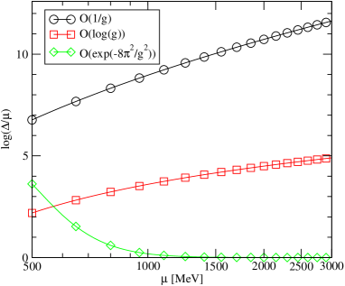
Figure 4: This figure shows successive terms in the perturbative expansion of $\log(\mu/\Delta)$ in QCD with $N_{f}=3$ flavors.

For $\mu\sim 500$ MeV the instanton term becomes comparable to the leading $O(1/g)$ term and we can no longer consider instantons effects to be a small correction. In this regime it probably makes more sense to do an instanton calculation and consider perturbative gluon exchanges as a correction. This is the approach originally suggested in [3, 4]. We should note, however, that for $\mu<500$ MeV the instanton calculation requires some phenomenological input because the instanton size distribution equ. (28) is no longer reliably calculable.

Ideally, we would like to check perturbative calculations of the gap against numerical calculations on the lattice. While this cannot be done in the realistic case of QCD with $N_{c}=3$ colors, the comparison is possible for QCD with $N_{c}=2$ colors and an even number of flavors, or for QCD with $N_{c}=3$ colors and a non-zero chemical potential for isospin rather than baryon number. In both of these cases it is also possible to separate the perturbative and instanton contributions by measuring both the gap and the mass of the $U(1)_{A}$ Goldstone boson [30].

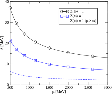
Figure 5: Numerical solution of the perturbative gap equation. We show the results with and without the fermion self energy included. We also show the asymptotic result, which corresponds to a reduction of the gap by a factor $\exp(-(\pi^{2}+4)/8)\simeq 0.18$.

7 Numerical Estimates

In this section we shall address a few more issues related to the magnitude of the gap. We will estimate the size of certain higher order corrections using numerical solutions of the gap equation. The first problem we wish to study is the importance of the fermion self energy correction. In Sect. 5 we saw that at asymptotically large chemical potential non-Fermi liquid effects in the fermion self energy reduce the gap by a factor $\exp(-(\pi^{2}+4)/8)\simeq 0.18$. In order to study the problem at moderate densities we consider the gap equation

$$\Delta(p_{4})=\frac{g^{2}}{18\pi^{2}}\int_{0}^{\mu}dq_{4}\,Z(q_{4})\frac{\Delta(q_{4})}{\sqrt{q_{4}^{2}+\Delta(q_{4})^{2}}}\log\left(\frac{b_{0}\mu}{|p_{4}^{2}-q_{4}^{2}|^{1/2}}\right),$$ (31)

with

$$Z(q_{4})=\left(1+\frac{g^{2}}{9\pi^{2}}\log\left(\frac{m_{D}}{q_{4}}\right)\right)^{-1}$$ (32)

and $b_{0}=256\pi^{4}g^{-5}$. If the density is very large then the scale inside the logarithm in equ. (32) does not matter. For our numerical estimates we have used the electric screening mass which is the scale suggested by one-loop calculations [24].

Figure 6: Numerical solution of the gap equation with running coupling constant effects included. We show the result with a fixed coupling $g=g(\mu)$, with a coupling that runs as a function of the momentum transfer as long as the momentum is larger than the electric screening scale, and a coupling that runs as a function of the momentum without any restrictions.

Numerical results are shown in Fig. 5. We observe that the gap is indeed reduced by the effects of fermion wave function renormalization, but at moderate density the reduction is smaller as compared to the asymptotic result. This is related to the fact that for $\mu\sim 500$ MeV and $\Delta\sim 50$ MeV the logarithm $\log(m_{D}/\Delta)$, which is formally $O(1/g)$, is numerically not very large.

The second issue we wish to address is the role of running coupling constant effects in the gap equation [31]. For the numerical estimates presented in the last section we have used the weak coupling result equ. (24) with the coupling constant evaluated at the scale $\mu$. It is easy to see that variation in the scale correspond to $O(g^{2})$ corrections, which is of the same order as other terms that have been neglected.

In order to estimate the size of these effects we consider the gap equation

$$\Delta(p_{4}) = \int_{0}^{\mu}dq_{4}\,\bigg{\{}\frac{g^{2}(m_{D})}{18\pi^{2}}\log\left(\frac{m_{D}^{3}+\Lambda_{M}^{3}}{\Lambda_{M}^{3}}\right)+2\log\bigg{(}\left[\frac{g^{2}(2\mu)}{g^{2}(m_{D})}\right]^{4/(3\beta_{0})}\bigg{)}\bigg{\}}$$ (33)

$$\mbox{}\hskip 28.45274pt\cdot Z(q_{4})\frac{\Delta(q_{4})}{\sqrt{q_{4}^{2}+\Delta(q_{4})^{2}}},$$

where $\Lambda_{M}=(\pi m_{D}^{2}|p_{4}\pm q_{4}|/4)^{1/3}$ is the scale that characterizes magnetic gluon exchanges. For momenta above the electric screening scale we have used the one-loop running coupling at the scale set by the momentum transfer. For momenta below the screening scale the coupling is frozen. In the language if the high density effective theory this means that the we have performed the matching at the electric screening scale. The four-fermion operator acquires an anomalous dimension which is equal to the QCD beta function [32]. Below the electric screening scale the gluonic interaction is effectively three-dimensional and does not run.

In Fig. 6 we show results obtained by solving equ. (33) numerically. For comparison we also show results obtained by solving a gap equation in which the coupling is allowed to run all the way down to the magnetic scale $(m_{D}^{2}\Delta)^{1/3}$. This approximation was suggested by Beane et al. [31]. We observe that for a moderate chemical potential $\mu\sim 500$ MeV the running coupling constant does not lead to very large effects. The reason is that there is no large hierarchy between the scales $m_{D}$ and $\mu$. If the chemical potential is very large, $\mu\sim 10$ GeV, the gap is increased by about 50%. This effect slowly disappears at asymptotically large chemical potential. The situation is different in case of the gap equation proposed by Beane et al. In that case the gap equation involves an extra large logarithm $\log(\mu/\Delta)$ and the pre-exponential factor in the asymptotic solution is modified [31].

8 Conclusions

We discussed an effective field theory for QCD at high baryon density. We studied, in particular, the problem of power counting in the high density effective theory. We showed that the power counting is complicated by “hard dense loops”, i.e. loop diagrams that involve the large scale $\mu^{2}$ and proposed a power counting that takes these effects into account. The modified $l$ counting implies that hard dense loops in gluon $n$-point functions have to be resummed below the scale $g\mu$, and that four fermion operators are leading order in the HDET power counting.

We used the high density effective theory to study the size of instanton corrections to the gap in superfluid quark matter. We found that instanton effects are very large in the regime $\mu\sim 500$ MeV which is of physical interest. We argued that numerical calculation in QCD with $N_{c}=2$ colors, or QCD with $N_{c}=3$ colors and non-zero isospin chemical potential, will of great help in determining the gap in $N_{c}=3$ QCD at non-zero baryon density. We also studied a renormalization group improved gap equation. We find no significant corrections as compared to a gap equation with a fixed coupling.

Acknowledgments: This work was supported in part by US DOE grant DE-FG-88ER40388.

References

- [1] D. Bailin and A. Love, Phys. Rept. 107, 325 (1984).
- [2] M. Alford, K. Rajagopal and F. Wilczek, Phys. Lett. B422, 247 (1998), [hep-ph/9711395].
- [3] R. Rapp, T. Schäfer, E. V. Shuryak and M. Velkovsky, Phys. Rev. Lett. 81, 53 (1998), [hep-ph/9711396].
- [4] M. Alford, K. Rajagopal and F. Wilczek, Nucl. Phys. B537, 443 (1999), [hep-ph/9804403].
- [5] T. Schäfer, Nucl. Phys. B 575, 269 (2000), [hep-ph/9909574].
- [6] K. Rajagopal and F. Wilczek, The condensed matter physics of QCD, in: Festschrift in honor of B.L. Ioffe, ’At the Frontier of Particle Physics / Handbook of QCD’, M. Shifman, ed., World Scientific, Singapore, [hep-ph/0011333].
- [7] M. Alford, Ann. Rev. Nucl. Part. Sci. 51, 131 (2001), [hep-ph/0102047].
- [8] G. Nardulli, Riv. Nuovo Cim. 25N3, 1 (2002), [hep-ph/0202037].
- [9] T. Schäfer, Quark Matter, BARC workshop on Quarks and Mesons; to appear in the proceedings, hep-ph/0304281.
- [10] D. H. Rischke, Prog. Part. Nucl. Phys. in press, nucl-th/0305030.
- [11] D. K. Hong, Phys. Lett. B 473, 118 (2000), [hep-ph/9812510].
- [12] D. K. Hong, Nucl. Phys. B 582, 451 (2000), [hep-ph/9905523].
- [13] T. Schäfer, Nucl. Phys. A 728, 251 (2003) [hep-ph/0307074].
- [14] T. Schäfer, Phys. Rev. D 65, 094033 (2002), [hep-ph/0201189].
- [15] E. Braaten and R. D. Pisarski, Phys. Rev. D 45, 1827 (1992).
- [16] E. Braaten, Can. J. Phys. 71, 215 (1993), [hep-ph/9303261].
- [17] R. Shankar, Rev. Mod. Phys. 66, 129 (1994).
- [18] J. Polchinski, hep-th/9210046.
- [19] D. T. Son, Phys. Rev. D 59, 094019 (1999), [hep-ph/9812287].
- [20] W. E. Brown, J. T. Liu and H. C. Ren, Phys. Rev. D61, 114012 (2000), [hep-ph/9908248].
- [21] W. E. Brown, J. T. Liu and H. C. Ren, Phys. Rev. D 62, 054016 (2000), [hep-ph/9912409].
- [22] B. Vanderheyden and J. Y. Ollitrault, Phys. Rev. D 56, 5108 (1997), [hep-ph/9611415].
- [23] W. E. Brown, J. T. Liu and H. c. Ren, Phys. Rev. D 62, 054013 (2000), [hep-ph/0003199].
- [24] C. Manuel, Phys. Rev. D 62, 076009 (2000), [hep-ph/0005040].
- [25] C. Manuel, Phys. Rev. D 62, 114008 (2000), [hep-ph/0006106].
- [26] D. Boyanovsky and H. J. de Vega, Phys. Rev. D 63, 034016 (2001), [hep-ph/0009172].
- [27] Q. Wang and D. H. Rischke, Phys. Rev. D 65, 054005 (2002), [nucl-th/0110016].
- [28] T. Schäfer, Phys. Rev. D 62, 094007 (2000), [hep-ph/0006034].
- [29] A. Schmitt, Q. Wang and D. H. Rischke, Phys. Rev. D 66, 114010 (2002), [nucl-th/0209050].
- [30] T. Schafer, Phys. Rev. D 67, 074502 (2003) [hep-lat/0211035].
- [31] S. R. Beane, P. F. Bedaque and M. J. Savage, Nucl. Phys. A 688, 931 (2001) [nucl-th/0004013].
- [32] T. Schäfer, in preparation.