TASI LECTURES ON PRECISION ELECTROWEAK PHYSICS

Abstract

hep-ph/0402031

UFIFT-HEP-03-11

CLNS 04/1862

January 2004

These notes are a written version of a set of lectures given at TASI-02 on the topic of precision electroweak physics.

1 Preliminary Remarks

Precision experiments have been crucial in both validating the Standard Model (SM) of particle physics and in providing directions in searching for new physics. The precision program, which started with the discovery of the weak neutral currents in 1973, has been extremely successful: it confirmed the gauge principle in the Standard Model, established the gauge groups and representations and tested the one-loop structure of the SM, validating the basic principles of renormalization, which in turn allowed for a prediction of the top quark and Higgs boson masses. In relation to new physics models, precision measurements have severely constrained new physics at the TeV scale and provided a hint of a possible (supersymmetric) gauge coupling unification at high energies.

1.1 What is it all about?

On the one hand, the term Precision Electroweak Physics (PEW) refers to quantities which are very well measured. How well? Let us say at the % level or better. However, not every well-measured quantity is of interest here. For example, the amount of cold dark matter in the Universe $\Omega_{CDM}$, Newton’s constant $G_{N}$ and the strong coupling constant $\alpha_{s}$ are all very well known, yet they do not belong to the electroweak sector of the Standard Model:

$$SU(3) \times SU(2)_{W}\times U(1)_{Y}$$

$${\rm QCD} {\rm~{}Electroweak}$$

The observables which are typically included in the precision electroweak data set are conveniently summarized in Tables 1.1 and 1.2.

Our goal in these lectures will be the following:

1. we shall learn the meaning of some of the quantities in Tables 1.1 and 1.2;

2. we shall find out how these quantities are measured by experiment;

3. we shall discuss the prospects for improving these measurements in the near future;

4. we shall find out their implications about the validity of the Standard Model;

5. we shall learn how they can be used to predict or constrain as yet undiscovered physics – for example, the mass of the Higgs boson, or the existence/lack of new physics beyond the Standard Model near the TeV scale.

Principal $Z$-pole observables, their experimental values, theoretical predictions using the SM parameters from the global best fit as of 1/03, and pull (difference from the prediction divided by the theoretical uncertainty). $\Gamma({\rm had})$, $\Gamma({\rm inv})$, and $\Gamma({\ell^{+}\ell^{-}})$ are not independent, but are included for completeness. From Ref. Langacker:2003tv. Quantity Group(s) Value Standard Model pull $M_{Z}$       [GeV] LEP $91.1876\pm 0.0021$ $91.1874\pm 0.0021$ $0.1$ $\Gamma_{Z}$        [GeV] LEP $2.4952\pm 0.0023$ $2.4972\pm 0.0011$ $-0.9$ $\Gamma({\rm had})$   [GeV] LEP $1.7444\pm 0.0020$ $1.7436\pm 0.0011$ — $\Gamma({\rm inv})$ [MeV] LEP $499.0\pm 1.5$ $501.74\pm 0.15$ — $\Gamma({\ell^{+}\ell^{-}})$ [MeV] LEP $83.984\pm 0.086$ $84.019\pm 0.027$ — $\sigma_{\rm had}$     [nb] LEP $41.541\pm 0.037$ $41.470\pm 0.010$ $1.9$ $R_{e}$ LEP $20.804\pm 0.050$ $20.753\pm 0.012$ $1.0$ $R_{\mu}$ LEP $20.785\pm 0.033$ $20.753\pm 0.012$ $1.0$ $R_{\tau}$ LEP $20.764\pm 0.045$ $20.799\pm 0.012$ $-0.8$ $A_{FB}(e)$ LEP $0.0145\pm 0.0025$ $0.01639\pm 0.00026$ $-0.8$ $A_{FB}(\mu)$ LEP $0.0169\pm 0.0013$ $0.4$ $A_{FB}(\tau)$ LEP $0.0188\pm 0.0017$ $1.4$ $R_{b}$ LEP + SLD $0.21664\pm 0.00065$ $0.21572\pm 0.00015$ $1.1$ $R_{c}$ LEP + SLD $0.1718\pm 0.0031$ $0.17231\pm 0.00006$ $-0.2$ $R_{s,d}/R_{(d+u+s)}$ OPAL $0.371\pm 0.023$ $0.35918\pm 0.00004$ $0.5$ $A_{FB}(b)$ LEP $0.0995\pm 0.0017$ $0.1036\pm 0.0008$ $-2.4$ $A_{FB}(c)$ LEP $0.0713\pm 0.0036$ $0.0741\pm 0.0007$ $-0.8$ $A_{FB}(s)$ DELPHI,OPAL $0.0976\pm 0.0114$ $0.1037\pm 0.0008$ $-0.5$ $A_{b}$ SLD $0.922\pm 0.020$ $0.93476\pm 0.00012$ $-0.6$ $A_{c}$ SLD $0.670\pm 0.026$ $0.6681\pm 0.0005$ $0.1$ $A_{s}$ SLD $0.895\pm 0.091$ $0.93571\pm 0.00010$ $-0.4$ $A_{LR}$ (hadrons) SLD $0.15138\pm 0.00216$ $0.1478\pm 0.0012$ $1.7$ $A_{LR}$ (leptons) SLD $0.1544\pm 0.0060$ $1.1$ $A_{\mu}$ SLD $0.142\pm 0.015$ $-0.4$ $A_{\tau}$ SLD $0.136\pm 0.015$ $-0.8$ $A_{e}(Q_{LR})$ SLD $0.162\pm 0.043$ $0.3$ $A_{\tau}({\mathcal{P}}_{\tau})$ LEP $0.1439\pm 0.0043$ $-0.9$ $A_{e}({\mathcal{P}}_{\tau})$ LEP $0.1498\pm 0.0048$ $0.4$ $Q_{FB}$ LEP $0.0403\pm 0.0026$ $0.0424\pm 0.0003$ $-0.8$

1.2 Useful references for further reading

For the current status of the precision electroweak observables, one should consult the “Electroweak model and constraints on New Physics” review [2] in the Particle Data Book [3]. There are nice lecture summaries from previous schools [4, 5, 6, 7, 8, 9, 10, 11], as well as book collections of relevant review articles [12, 13, 14]. The long-term prospects for improvement in the precision measurements have been discussed in several workshop reports, e.g. the Tevatron Run II Workshop [15] and Snowmass 2001 [16, 17, 18]. The website of the LEP Electroweak Working Group is another excellent source of information, with its continuously updated electroweak summary notes [20].

The recent status of non-$Z$-pole observables, as of 1/03. From Ref. Langacker:2003tv. Quantity Group(s) Value Standard Model pull $m_{t}$   [GeV] Tevatron $174.3\pm 5.1$ $174.4\pm 4.4$ $0.0$ $M_{W}$ [GeV] LEP $80.447\pm 0.042$ $80.391\pm 0.018$ $1.3$ $M_{W}$ [GeV] Tevatron,UA2 $80.454\pm 0.059$ $1.1$ $g_{L}^{2}$ NuTeV $0.30005\pm 0.00137$ $0.30396\pm 0.00023$ $-2.9$ $g_{R}^{2}$ NuTeV $0.03076\pm 0.00110$ $0.03005\pm 0.00004$ $0.6$ $R^{\nu}$ CCFR $0.5820\pm 0.0027\pm 0.0031$ $0.5833\pm 0.0004$ $-0.3$ $R^{\nu}$ CDHS $0.3096\pm 0.0033\pm 0.0028$ $0.3092\pm 0.0002$ $0.1$ $R^{\nu}$ CHARM $0.3021\pm 0.0031\pm 0.0026$ $-1.7$ $R^{\bar{\nu}}$ CDHS $0.384\pm 0.016\pm 0.007$ $0.3862\pm 0.0002$ $-0.1$ $R^{\bar{\nu}}$ CHARM $0.403\pm 0.014\pm 0.007$ $1.0$ $R^{\bar{\nu}}$ CDHS 1979 $0.365\pm 0.015\pm 0.007$ $0.3816\pm 0.0002$ $-1.0$ $g_{V}^{\nu e}$ CHARM II $-0.035\pm 0.017$ $-0.0398\pm 0.0003$ — $g_{V}^{\nu e}$ all $-0.041\pm 0.015$ $-0.1$ $g_{A}^{\nu e}$ CHARM II $-0.503\pm 0.017$ $-0.5065\pm 0.0001$ — $g_{A}^{\nu e}$ all $-0.507\pm 0.014$ $0.0$ $Q_{W}({\rm Cs})$ Boulder $-72.69\pm 0.44$ $-73.10\pm 0.04$ $0.8$ $Q_{W}({\rm Tl})$ Oxford/Seattle $-116.6\pm 3.7$ $-116.7\pm 0.1$ $0.0$ $10^{3}$ $\frac{\Gamma(b\rightarrow s\gamma)}{\Gamma_{SL}}$ BaBar/Belle/CLEO $3.48^{+0.65}_{-0.54}$ $3.20\pm 0.09$ $0.5$ $\tau_{\tau}$ [fs] direct/${\mathcal{B}}_{e}/{\mathcal{B}}_{\mu}$ $290.96\pm 0.59\pm 5.66$ $291.90\pm 1.81$ $-0.4$ $10^{4}$ $\Delta\alpha^{(3)}_{\rm had}$ $e^{+}e^{-}$/$\tau$ decays $56.53\pm 0.83\pm 0.64$ $57.52\pm 1.31$ $-0.9$ $10^{9}$ $(a_{\mu}-\frac{\alpha}{2\pi})$ BNL/CERN $4510.64\pm 0.79\pm 0.51$ $4508.30\pm 0.33$ $2.5$

2 The Tools of the Trade

As usual, we need to have a theory and experiments to test it. Before we go on to discuss the observables from Tables 1.1 and 1.2 in the next few sections, we first need to introduce the necessary theoretical ingredients and describe the relevant type of experiments. In Section 2.1 we review the electroweak Lagrangian and in Section 2.2 we discuss its input parameters. Sections 2.3 provides a general review of some of the types of experiments which have contributed to the results in Tables 1.1 and 1.2.

2.1 Theory

Achieving the remarkable precision displayed in Tables 1.1 and 1.2 is only possible because the Standard Model provides a well-defined theoretical framework for computing the different electroweak observables in terms of a few input parameters and thus predicting different relations among them.

The SM electroweak Lagrangian for fermions is given by

$${\mathcal{L}}_{F} = \sum_{i}\bar{\psi}_{i}\left(i/\!\!\!\partial-m_{i}-\frac{g_{i}m_{i}h}{2M_{W}}\right)\psi_{i}$$ (1)

$$- e\sum_{i}Q^{i}\bar{\psi}_{i}\gamma^{\mu}\psi_{i}A_{\mu}~{}~{}~{}(QED)$$ (2)

$$- \frac{g}{2\sqrt{2}}\sum_{i}\bar{\psi}_{i}\gamma^{\mu}(1-\gamma^{5})\left(T^{+}W^{+}_{\mu}+T^{-}W^{-}_{\mu}\right)\psi_{i}~{}~{}~{}(CC)$$ (3)

$$- \frac{g}{2\cos\theta_{W}}\sum_{i}\bar{\psi}_{i}\gamma^{\mu}(g_{V}^{i}-g_{A}^{i}\gamma^{5})\psi_{i}Z_{\mu}~{}~{}~{}(NC)$$ (4)

where the vector and axial vector couplings are

$$g_{V}^{i} = T_{3}^{i}-2Q^{i}\sin^{2}\theta_{W},$$ (5)

$$g_{A}^{i} = T_{3}^{i},$$ (6)

$Q^{i}$ is the electric charge of fermion $i$, $T_{3}^{i}$ is its weak isospin, $\theta_{W}$ is the Weinberg angle ($\tan\theta_{W}=g^{\prime}/g$), $g$ ($g^{\prime}$) is the $SU(2)_{W}$ ($U(1)_{Y}$) gauge coupling constant, and $e=g\sin\theta_{W}$ is the electromagnetic coupling constant. The photon ($A_{\mu}$) and Z-boson ($Z_{\mu}$) fields are given in terms of the hypercharge gauge boson $B_{\mu}$ and neutral $W$-boson $W^{3}_{\mu}$ as

$$A_{\mu} = B_{\mu}\cos\theta_{W}+W^{3}_{\mu}\sin\theta_{W},$$ (7)

$$Z_{\mu} = -B_{\mu}\sin\theta_{W}+W^{3}_{\mu}\cos\theta_{W}.$$ (8)

Often the neutral current interactions are equivalently written as

$$-\frac{g}{2\cos\theta_{W}}\sum_{i}\bar{\psi}_{i}\gamma^{\mu}\left(g_{L}^{i}(1-\gamma^{5})+g_{R}^{i}(1+\gamma^{5})\right)\psi_{i}Z_{\mu}~{}~{}~{}(NC)$$ (9)

with the redefinition

$$g_{V} = g_{L}+g_{R}$$ (10)

$$g_{A} = g_{L}-g_{R}$$ (11)

Exercise Use (5), (6), (7) and (8) to derive (1-4) from the $SU(2)_{W}\times U(1)_{Y}$ gauge theory lagrangian supplemented with the Yukawa terms for the fermions. Hint: you will need to know the Higgs vacuum expectation value $v$, which is computed by minimizing the tree-level Higgs potential

$$V_{H}=-\frac{1}{2}\mu^{2}h^{2}+\frac{\lambda_{H}}{4}h^{4}$$ (12)

as

$$v=\sqrt{\frac{\mu^{2}}{\lambda_{H}}}.$$ (13)

2.2 Fundamental parameters, input parameters and observables

Fundamental parameters are the parameters appearing in the original gauge theory Lagrangian. In the case of the electroweak Lagrangian, the fundamental parameters are the gauge couplings $g^{\prime}$ and $g$. The Higgs sector of the theory (12) adds two more fundamental parameters: the Higgs mass parameter $\mu$ and self-coupling $\lambda_{H}$. The remaining fundamental parameters are the Yukawa couplings in the Yukawa sector (1). Putting all together, the set of fundamental parameters is

$$\{g,g^{\prime},\lambda_{H},\mu^{2},\lambda_{i}\}.$$ (14)

Often, as was the case above in Eq. (1-4), it is convenient to rewrite the Lagrangian in terms of derived quantities, i.e. input parameters. Through a simple redefinition we can trade one fundamental parameter for a combination of a new (input) parameter and the remaining fundamental parameters, e.g.

$$g^{\prime}=g\tan\theta_{W}$$ (15)

eliminates $g^{\prime}$ from the Lagrangian and replaces it with $\theta_{W}$. Another example is

$$v=\frac{2M_{W}}{g},$$ (16)

which eliminates the combination $v=\mu/\sqrt{\lambda_{H}}$ in favor of the $W$-boson mass $M_{W}$. The latter is directly accessible experimentally, unlike either $\lambda_{H}$ or $\mu$. A similar trick allows to go from Yukawa couplings to fermion masses:

$$\lambda_{i}=\frac{gm_{i}}{\sqrt{2}M_{W}},$$ (17)

which is very convenient, as most fermion masses are well-known experimentally while in contrast the Yukawa couplings are small (with the exception of the top Yukawa) and thus difficult to measure. Of course, one should make sure the total number of parameters stays the same for both the fundamental and input parameters.

For the precision electroweak tests of the SM the following set of well-measured input parameters is typically used:

$$\{\alpha,G_{F},M_{Z},m_{h},m_{i}\},$$ (18)

where $\alpha=e^{2}/4\pi$ is the fine structure constant, $G_{F}$ is the Fermi constant, which is measured from the muon lifetime, and $M_{Z}$ ($m_{h}$) is the $Z$-boson (Higgs boson) mass.

Exercise Find the relation between the input parameter set (18) and the fundamental parameter set (14).

Finally, observables are the quantities which are measured by experiment. An example is the set of electroweak observables listed in Tables 1.1 and 1.2. If the number of observables is larger than the number of input parameters, we can test the model.

2.3 Experimental facilities

As can be seen from Tables 1.1 and 1.2, the electroweak observables have been measured at a variety of experimental facilities. We shall now briefly describe each type.

Lepton colliders

Lepton ($e^{+}e^{-}$) colliders have played a very important role in the precision program. Lepton colliders have numerous advantages, perhaps best summarized in the following aphorism: “At a lepton collider, every event is signal. At a hadron collider, every event is background.” The main attractive features are:

• Fixed center of mass energy in each event. This provides an additional kinematic constraint, useful for eliminating the backgrounds as well as extracting properties of new particles, allowing e.g. a missing mass measurement.

• All of the available beam energy is used (minus beamstrahlung), i.e. we have an efficient use of particle acceleration.

• Clean environment: easier identification of the underlying physics in the event, easier heavy flavor tagging, less backgrounds.

• Polarizability of the colliding beams (SLC). The polarization of the colliding beams can be used to reweight the contribution of the different diagrams involving $W$’s, $Z$’s and $\gamma$’s.

Naturally, lepton colliders also have certain disadvantages in comparison to hadron colliders (see below), which makes both types of facilities equally valuable and to a large extent complementary.

Figure 1: Total $e^{+}e^{-}$ cross section from CESR/DORIS to LEP energies.

Figure 1 summarizes some of the history of $e^{+}e^{-}$ colliders. In reverse chronological order (including future facilities), they are:

• The Next Linear Collider (NLC) with an initial CM energy of 500 GeV is now under active discussion as the next large international particle physics facility. Its timescale is still uncertain, but the NLC was ranked as the top priority among mid-term science facilities in the Department of Energy’s Office of Science 20-year science facility plan [21].

• LEP-II at CERN (1996-2000). It had the highest CM energy so far among lepton colliders. LEP-II took data at several $\sqrt{s}$ before shutting down in November 2000 amidst much speculation and heated discussions. There were four experiments (detectors) at diametrically opposite sites: ALEPH, DELPHI, L3 and OPAL.

• LEP-I at CERN (1989-1995), which took data at several energies around $\sqrt{s}=M_{Z}$.

• SLC at SLAC (1989-1998). It reached energies up to 100 GeV and also took data around the $Z$-pole. Unlike LEP, it had an important advantage: the availability of beam polarization (80%).

• B-factories: PEP-II at SLAC (1999-present), $9\times 3.1$ GeV; KEKB at KEK (Japan) (1999-present) $8\times 3.5$ GeV; CESR at Cornell (1979-present). Exercise: Why are the B-factories asymmetric?

• Others ($\sqrt{s}<10$ GeV) (Novosibirsk, Bejing, Frascati).

Hadron colliders

In turn, hadron colliders have their own advantages:

• Protons are much heavier than electrons, which leads to a reduction in the radiation losses. As a result, for a given CM energy, the ringsize of a hadron collider is smaller. Equivalently, for a given ringsize (and fixed magnetic field), a hadron collider allows to reach higher CM energies.

• Even though the CM energy of the colliding beams is large, the typical parton CM energy is much smaller, but usually still beyond the CM energy of LC competitors.

The main hadron collider facilities are the following:

• LHC (CERN) is currently under construction and is projected to begin operation in 2007-8 as a $7\times 7$ TeV $pp$ collider. There will be four experiments – ATLAS, CMS, LHCB and ALICE. The initial data taking rate will be 10 ${\rm fb}^{-1}$ per year at low luminosity and will subsequently increase to 100 ${\rm fb}^{-1}$ per year.

• The Tevatron Run II at Fermilab is now operating as a $0.98\times 0.98$ $p\bar{p}$ TeV collider. There are two experiments: CDF and D0, and the hope nowadays is for 8 ${\rm fb}^{-1}$ per experiment before the LHC.

• The Tevatron Run I (1987-1996): discovered the top quark. It operated in a $0.9\times 0.9$ $p\bar{p}$ mode and delivered 110 ${\rm pb}^{-1}$ of data per experiment.

• $Sp\bar{p}S$ at CERN (1981-1990). It was a $300\times 300$ GeV $p\bar{p}$ collider, and discovered the $W$ and $Z$ bosons.

It is interesting that the last three SM particles ($W$, $Z$ and $t$) were discovered at hadron colliders and chances are that the last one (the Higgs boson) will follow suit.

Other facilities

In addition to the collider experiments mentioned above, there are numerous fixed target experiments, whose main advantage is the lower cost and large luminosity (because of the dense target). Their main disadvantage is the low center of mass energy, which scales with the beam energy $E_{b}$ only as $E_{CM}\sim\sqrt{E_{b}}$. Another class of experiments on muon dipole moments were done at muon storage rings – at CERN, and more recently, at BNL.

In conclusion of this section, we should comment on the experimental identification of heavy particles, which decay promptly and are detected only through their decay products. For example, a $W$-boson decays either to a pair of quarks, which later materialize into QCD jets, or to a lepton and the corresponding neutrino. The $W$ branching fractions are $B(W\rightarrow qq^{\prime})\sim 2/3$, and $B(W\rightarrow\ell\nu_{\ell})\sim 1/9$ for $\ell=e,\mu,\tau$. The jets (or the lepton and its neutrino) may have had a different source, and the only indication that they may have come from a $W$ decay is that their invariant mass is close to $M_{W}$.

Similarly, a $Z$-boson can decay to pairs of quarks, leptons or neutrinos, with branching fractions $B(Z\rightarrow q\bar{q})\sim 0.7$, $B(Z\rightarrow\nu\bar{\nu})\sim 0.2$ and $B(Z\rightarrow\ell^{+}\ell^{-})\sim 0.1$ (summed over the three generations). When both decay products are visible, their invariant mass is again required to be near $M_{Z}$.

A word of caution: $\tau$ is not always a lepton! A $\tau$-lepton can decay leptonically to $e$ or $\mu$ with a branching ratio $0.18$ for each, or hadronically, with a branching ratio 0.64. In the latter case it appears as a “tau jet”, which is similar to an ordinary QCD jet. To an experimentalist, a “lepton” is either an $e$ or a $\mu$, which may or may not have come from a tau decay. By $\tau$’s, experimentalists often mean “tau jets”.

3 Precision Measurements at the $Z$ Pole

At the $Z$ pole the cross-section for $e^{+}e^{-}\rightarrow f\bar{f}$ is dominated by the $Z$ diagram. For $f\neq e$ we have

$$\frac{d\sigma_{Z}^{f}}{d\Omega}=\frac{9}{4}\frac{s\Gamma_{ee}\Gamma_{f\bar{f}}/M_{Z}^{2}}{(s-M_{Z}^{2})^{2}+s^{2}\Gamma^{2}_{Z}/M_{Z}^{2}} \biggl{[} (1+\cos^{2}\theta)(1-P_{e}A_{e})$$ (19)

$$+ 2\cos\theta A_{f}(-P_{e}+A_{e})\biggr{]}$$

where $P_{e}$ is the polarization of the electron beam (relevant at SLC), $s$ is the square of the CM energy, $\Gamma_{Z}$ is the total $Z$ width, $\Gamma_{ee}$ and $\Gamma_{f\bar{f}}$ are the partial widths for $Z\rightarrow ee$ and $Z\rightarrow f\bar{f}$, correspondingly. (The partial widths are related to the $Z$ branching fractions as $B(Z\rightarrow f\bar{f})=\Gamma_{f\bar{f}}/\Gamma_{Z}$.) In (19) $\theta$ is the angle between the incident electron and the outgoing fermion and $A_{f}$ is the left-right coupling constant asymmetry:

$$A_{f}=\frac{2g_{V}^{f}g_{A}^{f}}{(g_{V}^{f})^{2}+(g_{A}^{f})^{2}}=\frac{(g_{L}^{f})^{2}-(g_{R}^{f})^{2}}{(g_{L}^{f})^{2}+(g_{R}^{f})^{2}}$$ (20)

where in the second equation we have used (5) and (6). Notice that $A_{f}\leq 1$. Since $g_{V}$ and $g_{A}$ only depend on the quantum numbers of the particles, it follows that $A_{f}$ is the same for all charged leptons, all up-type quarks and all down-type quarks. For example, for charged leptons

$$g_{V}^{\ell} = -\frac{1}{2}-2(-1)\sin^{2}\theta_{W}\sim-0.50+0.462=-0.038$$ (21)

$$g_{A}^{\ell} = -\frac{1}{2}=-0.50$$ (22)

We see that because of an accidental cancellation $g_{V}^{\ell}\ll g_{A}^{\ell}$. For the asymmetry we then get (at tree level)

$$A_{\ell}=\frac{2(-0.038)(-0.5)}{(-0.038)^{2}+(-0.5)^{2}}\sim 0.15$$ (23)

(compare to the values measured in Table 1.1). This small value of $A_{\ell}$ makes it particularly sensitive to electroweak vacuum polarization corrections (which have an impact on $\sin^{2}\theta_{W}$). In terms of $\sin^{2}\theta_{W}$, we have

$$A_{\ell}=\frac{2(1-4\sin^{2}\theta_{W})}{1+(1-4\sin^{2}\theta_{W})^{2}}.$$ (24)

Therefore small changes in $\sin^{2}\theta_{W}$ are amplified by a factor of 8 in the leptonic asymmetry $A_{\ell}$.

Exercise: Confirm roughly the numerical values for $A_{b}$ and $A_{c}$ in Table 1.1.

Let us now discuss the various measurements on the $Z$-pole. We shall need the following integrals for the forward and backward regions:

$$F :\quad\int_{0}^{\pi/2}(1+\cos^{2}\theta)\sin\theta d\theta=\frac{4}{3};\qquad\int_{0}^{\pi/2}2\cos\theta\sin\theta d\theta=1;$$ (25)

$$B :\quad\int_{\pi/2}^{\pi}(1+\cos^{2}\theta)\sin\theta d\theta=\frac{4}{3};\qquad\int_{\pi/2}^{\pi}2\cos\theta\sin\theta d\theta=-1.$$ (26)

3.1 $Z$ resonance parameters

Scanning the $Z$ peak and fitting to $\sigma_{Z}^{f}$ yields measurements of $M_{Z}$, $\Gamma_{Z}$ and the peak hadronic ($f=q$) total cross-section $\sigma_{had}$ (obtained for $s=M_{Z}^{2}$ by integrating (19) over the full solid angle):

$$\sigma_{had}=12\pi\frac{\Gamma_{ee}\Gamma_{had}}{M_{Z}^{2}\Gamma_{Z}^{2}}.$$ (27)

Recall that the LEP beams are not polarized, so $P_{e}=0$. Figure 2 shows the hadronic cross-section $\sigma_{had}$ measured by the four collaborations as a function of the center-of-mass energy (solid line). Also shown as a dashed line is the cross-section after unfolding all effects due to photon radiation. The radiative corrections are large but very well known. At the peak the QED deconvoluted cross-section is 36% larger and the peak position is shifted by $\sim 100$ MeV.

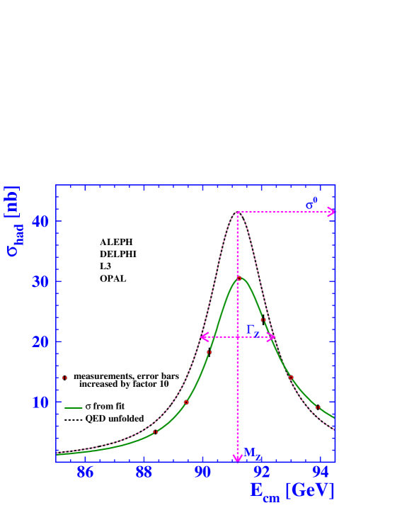
Figure 2: The final hadronic cross-section averaged over the four experiments at LEP-I, as a function of the center-of-mass energy, as measured (solid line) and QED deconvoluted (dashed line).

3.2 Branching ratios and partial widths

Looking at various exclusive final states one can determine the following ratios

$$R_{\ell} \equiv \frac{\Gamma_{had}}{\Gamma_{\ell}}\sim\frac{0.7}{0.0333}\sim 21;$$ (28)

$$R_{b} \equiv \frac{\Gamma_{bb}}{\Gamma_{had}};$$ (29)

$$R_{c} \equiv \frac{\Gamma_{cc}}{\Gamma_{had}};$$ (30)

with $\ell=\{e,\mu,\tau\}$. Basically this amounts to measuring the $Z$ branching fractions.

Having measured the total width from the peak scan and all visible partial widths, one can determine the invisible partial width (for $Z\rightarrow\nu\bar{\nu}$):

$$\Gamma_{inv}=\Gamma_{Z}-\Gamma_{had}-\Gamma_{ee}-\Gamma_{\mu\mu}-\Gamma_{\tau\tau}$$ (31)

and count the number of neutrino species $N_{\nu}$ coupling to the $Z$. Assuming that $\Gamma_{inv}=N_{\nu}\Gamma_{\nu}$, where $\Gamma_{\nu}$ is the $Z$ partial width to pairs of a single neutrino species, we have

$$N_{\nu}=\frac{\Gamma_{inv}/\Gamma_{\ell}}{\left(\Gamma_{\nu}/\Gamma_{\ell}\right)_{SM}}.$$ (32)

The ratio of $\Gamma_{inv}$ and the $Z$ partial width into charged leptons is used in order to minimize the uncertainties due to the electroweak corrections which are common to both partial widths and cancel out in their ratio. The $Z$ lineshape in the hadronic channel is shown in Figure 3 along with the SM prediction for two, three or four neutrinos species. The result confirms that there are three light neutrino flavors with SM-like couplings to the $Z$.

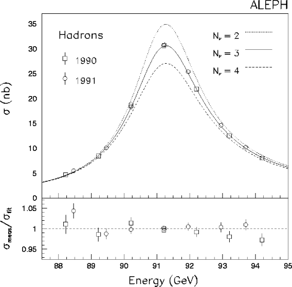
Figure 3: The $Z$ lineshape in the hadronic channel along with the SM prediction for two, three or four neutrinos species [23]. The lower plot shows the ratio of the measured points to the best-fit values.

3.3 Unpolarized forward-backward asymmetry

The unpolarized forward-backward asymmetry is determined by a simple counting method in $e^{+}e^{-}\rightarrow f\bar{f}$ scattering

$$A_{FB}^{f}\equiv\frac{\sigma_{F}^{f}-\sigma_{B}^{f}}{\sigma_{F}^{f}+\sigma_{B}^{f}}=\frac{3}{4}A_{e}A_{f},$$ (33)

where $\sigma_{F}^{f}$ ($\sigma_{B}^{f}$) is the total cross-section for forward (backward) scattering of $f$ with respect to the incident $e^{-}$ direction.

Exercise: Use (25-26) in order to derive the second equality in (33) and then check the numerical values for $A_{FB}^{f}$ from Table 1.1 for $f=\ell,b,c$.

3.4 Left-right asymmetry

The left-right asymmetry is defined as

$$A_{LR}^{f}\equiv\frac{1}{P_{e}}\frac{\sigma^{f}(-|P_{e}|)-\sigma^{f}(+|P_{e}|)}{\sigma^{f}(-|P_{e}|)+\sigma^{f}(+|P_{e}|)}=A_{e},$$ (34)

where $\sigma^{f}(P_{e})$ is the total (integrated over all angles) cross-section for producing $f\bar{f}$ pairs with an electron beam of polarisation $P_{e}$.

Exercise: Derive the second equality.

3.5 Left-right forward-backward asymmetry

The left-right forward-backward asymmetry is defined as

$$\bar{A}_{FB}^{f}\equiv\frac{\sigma^{f}_{F}(-|P_{e}|)-\sigma_{B}^{f}(-|P_{e}|)-\sigma^{f}_{F}(+|P_{e}|)+\sigma_{B}^{f}(+|P_{e}|)}{\sigma^{f}_{F}(-|P_{e}|)+\sigma_{B}^{f}(-|P_{e}|)+\sigma^{f}_{F}(+|P_{e}|)+\sigma_{B}^{f}(+|P_{e}|)}=\frac{3}{4}P_{e}A_{f}.$$ (35)

It allows a direct determination of the $A_{f}$ quantities which are presented in Table 1.1.

Exercise: Derive the second equality.

To summarize or discussion so far, there are three observable asymmetries, measuring either $A_{e}$, $A_{f}$ or their product.

3.6 Tau polarization

The tau lepton is the only fundamental fermion whose polarization is experimentally accessible at LEP and SLC. The average polarization of $\tau$ leptons is defined by

$$P_{\tau}(s)=\frac{\sigma^{tot}_{+}(s)-\sigma^{tot}_{-}(s)}{\sigma^{tot}(s)},$$ (36)

where $\sigma^{tot}(s)$ is the $\tau$ production cross-section via $Z$ exchange, integrated over all angles, and the subscripts $+$ and $-$ refer to the $\tau$ helicity states $+1$ and $-1$. The dependence of $P_{\tau}$ at the $Z$ pole on the polar angle $\theta$ has the form [24]

$$P_{\tau}(\cos\theta)=-\frac{A_{\tau}(1+\cos^{2}\theta)+2A_{e}\cos\theta}{1+\cos^{2}\theta+2A_{\tau}A_{e}\cos\theta}.$$ (37)

The $\tau$ polarization is measured using five exclusive decay modes which comprise about 80% of all $\tau$ decays: $e\nu\bar{\nu}$, $\mu\nu\bar{\nu}$, $\pi(K)\nu$, $\rho\nu$ and $a_{1}\nu$. The single $\pi$ and $K$ modes are not normally distinguished. The different channels do not all have the same sensitivity to the $\tau$ polarization, $\pi(K)\nu$ being the best in that respect (see Fig. 4). The energy and/or angular distributions of the decay products can be used as $\tau$ polarization analysers [25]. Figure 4 shows an example of the different distributions used and their sensitivity to the $\tau$ polarization.

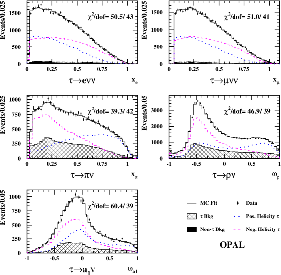
Figure 4: Observed distributions of the polarization estimators for the different channels studied by OPAL [26], compared to the SM expectation for positive or negative $\tau$ helicity.

Fitting the experimental data for $P_{\tau}(\cos\theta)$ (an example from the ALEPH experiment [27] is shown in Figure 5) to Eq. (37) allows an extraction of $A_{\tau}$ and $A_{e}$ which enter Table 1.1 as $A_{\tau}({\mathcal{P}}_{\tau})$ and $A_{e}({\mathcal{P}}_{\tau})$, correspondingly.

Figure 5: Tau polarization as a function of $\cos\theta$. The dashed (dotted) line is the result from a global fit to the data with (without) the universality assumption ${\mathcal{A}}_{e}={\mathcal{A}}_{\tau}$.

4 Precision Measurements at LEP-II

LEP-II was able to pair produce $W$’s and perform measurements of $M_{W}$, $\Gamma_{W}$ and the $W$ branching fractions. There are three diagrams contributing to $W$-pair production: a $t$-channel $\nu$ exchange, and an $s$-channel $\gamma^{\ast}$ and $Z$ exchange. The latter two diagrams contain triple gauge boson couplings, therefore LEP also tested the nonabelian nature of the SM gauge interactions.

The $W$ mass measurement involves reconstruction of the invariant mass of the $W$ decay products. For $WW$, there are three possible final states: $4q$, $qq\ell\nu_{\ell}$ and $2\ell 2\nu_{\ell}$. The LEP measurements used only the first two channels. In the case of $qq\ell\nu_{\ell}$, the energy and momentum of the missing neutrino are easily deduced from energy and momentum conservation. Then the four objects are paired up and the invariant mass of each pair is computed. The resulting invariant mass distribution in the $qq\mu\nu_{\mu}$ channel is shown in Figure 6.

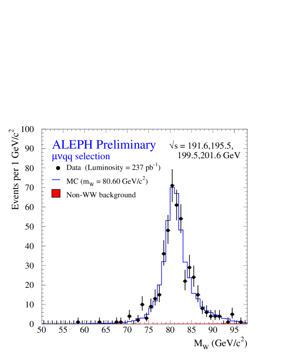
Figure 6: Reconstructed $W$ mass distribution from the ALEPH experiment for the $qq\mu\nu_{\mu}$ channel. The data are compared to the Monte Carlo prediction for $M_{W}=80.60$ GeV.

The mass peak is very pronounced, with virtually no background. The position of the peak allows an extraction of $M_{W}$, while its width is indicative of $\Gamma_{W}$, where in addition one has to worry about detector resolution effects (smearing). All four experiments are consistent and so far the LEP $M_{W}$ measurement is slightly better than the $M_{W}$ measurement from the Tevatron (see below). The $W$ mass measurement is of extreme importance - as we shall see later, $M_{W}$ is one of the observables most sensitive to the Higgs mass $m_{h}$.

The $W$ branching ratios were measured in $WW$ production and the results displayed in Table 4 nicely demonstrate lepton universality.

LEP measurements of the $W$ branching fractions derived from $WW$ production cross-section measurements[20]. Decay mode Branching fraction (%) $W\rightarrow e\nu_{e}$ $10.59\pm 0.17$ $W\rightarrow\mu\nu_{\mu}$ $10.55\pm 0.16$ $W\rightarrow\tau\nu_{\tau}$ $11.20\pm 0.22$ $W\rightarrow qq^{\prime}$ $67.77\pm 0.28$

The measurement of the rise in the $W$-pair cross-section near threshold provides an alternative method for determining $M_{W}$. The result for energies up to 207 GeV is shown in Figure 7. The method is statistically limited and yields inferior precision compared to direct $M_{W}$ reconstruction. However, it clearly demonstrates the need for all triple gauge boson couplings in order to understand the data.

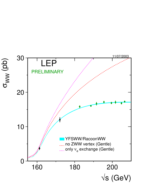
Figure 7: The measured $WW$ cross-section at LEP as a function of the center-of-mass energy, compared to the predictions of the event generators RacoonWW and YFSWW. The magenta (upper dotted) line is the theoretical result ignoring both $WW\gamma$ and $WWZ$ couplings, while the red (lower dotted) line neglects $WWZ$ only.

LEP-II also measured the $ZZ$ cross-section. However, the electron couplings to the $Z$ are smaller, and in addition $M_{Z}>M_{W}$. Thus the sample of $ZZ$ pairs was much smaller and the measurement of the $ZZ$ cross-section was not as good as for the $WW$ case. Nevertheless, a comparison of the combined data to theory (Fig. 8) reveals good agreement within the large errors of the data.

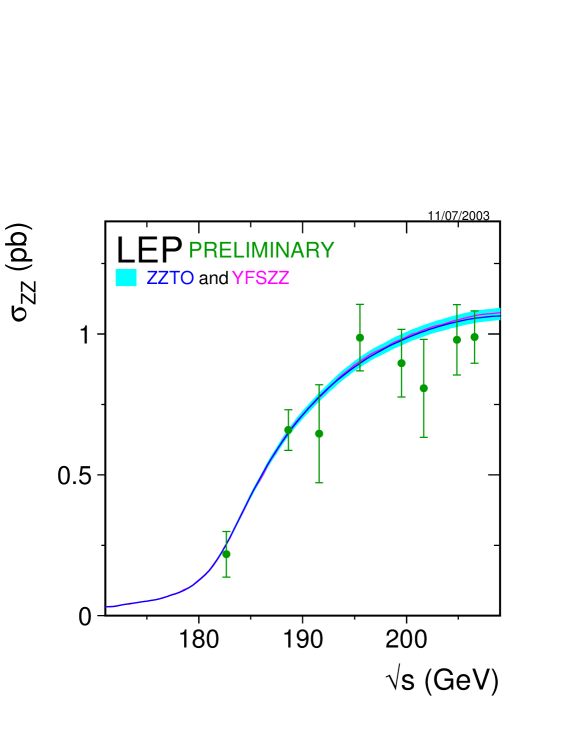
Figure 8: The measured $e^{+}e^{-}\to ZZ$ cross-section at LEP as a function of the center-of-mass energy. The solid line is the SM prediction and the band indicates its $\pm 2\%$ uncertainty.

5 Precision Measurements at the Tevatron

5.1 Top mass measurement

Since the top quark is so heavy, so far it can only be produced at the Tevatron. The dominant mechanism for pair-production is $q\bar{q}\rightarrow t\bar{t}$ through a virtual $s$-channel gluon. Single top production is also possible.

The top quark decays as $t\rightarrow Wb$ almost 100% of the time. Top quark pair-production then gives $W^{+}W^{-}b\bar{b}$ events and there are three possible discovery channels, depending on the $W$ decays:

• Both $W$’s decaying hadronically - 6 jet final state ($2b4j$). This is the largest signal cross-section, but with large QCD backgrounds.

• One $W$ decays hadronically, the other leptonically: $\ell 2b2j\mbox{${E\!\!\!/}_{T}$}$ (lepton plus jet sample). This was the best channel for Run I, because there was a sufficient number of events, yet the background was under control.

• Both $W$’s decaying leptonically: $2\ell 2b\mbox{${E\!\!\!/}_{T}$}$ (dilepton sample). This channel has the largest $S/\sqrt{B}$ ratio, however it is limited by statistics.

Both experiments (CDF and D0) have conducted measurements of $m_{t}$ in Run I and the results from the two experiments as well as from different channels are consistent with each other (see Fig. 9).

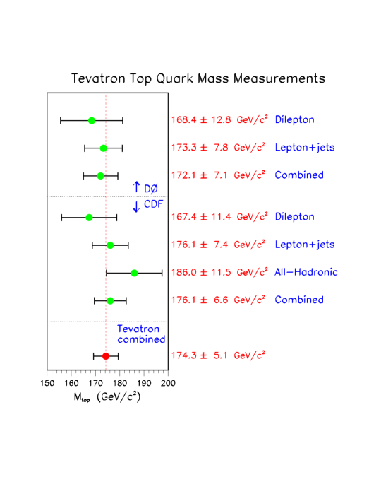
Figure 9: Run I Tevatron results for $m_{t}$ and the global average. (From Ref. Chakraborty:2003iw.)

The direct $m_{t}$ measurements from the Teavtron are in very good agreement with the best fit value for $m_{t}$ extracted from the electroweak precision fits (see Section 6.6). Right now $m_{t}$ is the best measured of all quark masses.

In Run II one can anticipate significant improvements – the expected precision on the $m_{t}$ measurements is shown in Table 5.1. In fact, there are already some preliminary top results from Run II [29].

Expected precision (in GeV) on the $m_{t}$ measurements in Run II for the lepton plus jet and for the dilepton channel. (From Ref. Baur:2002gp.) $\int{\mathcal{L}}dt$ (${\rm fb}^{-1}$) 2 15 30 Statistical 1.7 0.63 0.44 $bb\ell jj\mbox{${E\!\!\!/}_{T}$}$ Systematic 2.1 1.2 1.1 Total 2.7 1.3 1.2 Statistical 2.4 0.87 0.62 $bb2\ell\mbox{${E\!\!\!/}_{T}$}$ Systematic 1.4 1.0 1.0 Total 2.8 1.3 1.2

5.2 $W$ mass measurement

$W$ bosons can be singly produced at the Tevatron with a relatively large cross-section $\sim 1$ nb. The $W$ is subsequently detected through its leptonic decay mode to a charged lepton and the corresponding neutrino. (The hadronic decays cannot be used because of the enormous dijet background from QCD.) The signature is $\ell\mbox{${E\!\!\!/}_{T}$}+X$. Unfortunately, we cannot reconstruct the invariant mass of the $W$, because of the unknown longitudinal component of the neutrino momentum. Hence we must extract $M_{W}$ from transverse quantities only.

There are several possible methods [30]: looking at the transverse mass ($M_{T}^{W}$), the transverse momentum of the charged lepton ($p_{T}^{\ell}$) or the missing transverse energy ${E\!\!\!/}_{T}$. Since different methods have different systematic errors, it is desirable to have as many independent measurements as possible.

In Run I the transverse mass method was used. (The $p_{T}^{\ell}$ method was limited by the number of leptonic $Z$ events – see below.) The transverse mass is defined as

$$M_{T}^{W}=\sqrt{2p_{T}^{\ell}p_{T}^{\nu}(1-\cos\phi)}$$ (38)

where $\phi$ is the angle between $\vec{p}_{T}^{\ell}$ and $\vec{p}_{T}^{\nu}$ in the transverse plane. $\vec{p}_{T}^{\nu}$ is nothing but the missing transverse energy and is measured as

$$\vec{p}_{T}^{\nu}=-(\vec{U}+\vec{p}_{T}^{\ell})$$ (39)

where $U$ is total transverse momentum of the remaining hadronic activity in the event (typically a jet from initial state radiation). The transverse mass distribution exhibits a characteristic drop-off around $M_{W}$, as shown in Fig. 10.

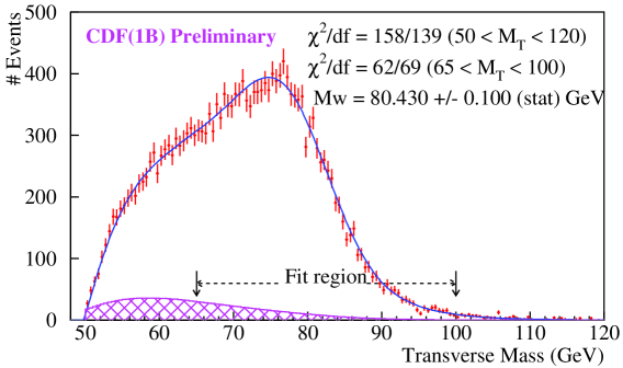
Figure 10: Transverse mass distribution of $W\to\mu\nu$ events from the CDF Run IB data, with the best fit. The shaded distribution is the background.

The $M_{W}$ measurement is done by fitting Monte Carlo predictions for different values of $M_{W}$ to the observed $M_{T}^{W}$ distribution. In addition, at large $M_{T}^{W}$ the shape of the distribution is sensitive to the intrinsic $W$ width $\Gamma_{W}$, as illustrated in Fig. 11, which allows for a direct measurement of $\Gamma_{W}$:

$$\Gamma_{W}=2.055\pm 0.125\ GeV.$$ (40)

Figure 11: Monte Carlo simulations of the transverse mass spectrum for different $W$-boson widths. The normalization is arbitrary. (From Ref. Abazov:2002xj.)

An alternative method for measuring $M_{W}$ employs the lepton $p_{T}$ distribution, which cuts off around $M_{W}/2$. However, unlike $M_{T}^{W}$, the $p_{T}^{\ell}$ distribution depends on the $W$ boost, and therefore on the transverse momentum $p_{T}^{W}$ with which the $W$ was produced. It is difficult to compute $p_{T}^{W}$ by theoretical means, especially in the low $p_{T}$ region, and it is best to extract it from data. For this purpose the Tevatron experiments have used the observed $p_{T}^{Z}$ distribution, which has a similar shape, but fewer events. Hence, in Run I this method was statistically limited, but offers good prospects for Run II. The expected precision of the $M_{W}$ measurements at the Tevatron by the two methods is shown in Table 5.2.

Expected precision (in MeV) on the Tevatron $M_{W}$ measurements in Run II. (From Ref. Baur:2002gp.) $\int{\mathcal{L}}dt$ (${\rm fb}^{-1}$) 2 15 30 Statistical 19 7 5 $M_{T}^{W}$ Systematic 19 16 15 Total 27 17 16 Statistical 44 16 11 $p_{T}^{\ell}$ Systematic 10 4 3 Total 44 16 12

6 Theoretical Interpretation of the Precision Electroweak Data

We can make use of the precision electroweak data in three differrent ways:

• Test the Standard Model.

• Predict the preferred mass range of yet undiscovered particles: top quark in the past, nowadays the Higgs boson.

• Point towards specific new physics models (in case of some discrepancy) or constrain new physics models (if agreement is found).

We shall discuss each one in turn.

6.1 Testing the Standard Model

Having made a variety of measurements for different observables, we can test the SM by comparing theory to experiment. For this purpose we need to compute the theoretical prediction within the SM for each observable. How do we do it?

Recall that in the SM we start with the input parameters

$$\left\{p\right\}\equiv\left\{\alpha,G_{F},M_{Z},g_{3},m_{h},m_{t},m_{b},m_{c},m_{s},...\right\},$$ (41)

where the first three are the parameters of the electroweak sector. Any other electroweak quantity, e.g. $\sin^{2}\theta_{W}$, $M_{W}$ etc. can be expressed in terms of these and thus is predicted by the model. At tree level the expressions are simple and only involve the electroweak inputs $\alpha,G_{F},M_{Z}$, e.g. the Weinberg angle can be found from

$$\sin 2\theta_{W}=\left(\frac{2\sqrt{2}\pi\alpha}{G_{F}M_{Z}^{2}}\right)^{1/2}.$$ (42)

Similarly, the $W$ mass is

$$M_{W}=M_{Z}\cos\theta_{W}$$ (43)

with $\theta_{W}$ given by (42).

The radiative corrections, however, modify the tree level relations and introduce the remaining (non-electroweak) parameters into the game, so that each electroweak observable depends in principle on the full set of input parameters (41):

$${\mathcal{O}}_{i}^{theory}(\{p\})={\mathcal{O}}_{i}^{tree}(\alpha,G_{F},M_{Z})\left[1+\Delta_{i}(\{p\})\right].$$ (44)

By measuring enough electroweak observables (with sufficient precision so that we are sensitive to the radiative corrections) we can extract information about the values of the other parameters outside the electroweak sector. We can then test the model for consistency by comparing the values deduced indirectly with direct measurements of those parameters.

So the strategy is as follows. First compute the corrections in a certain renormalization scheme, treating some parameters as fixed inputs (usually the best measured ones). Then perform a global fit to the electroweak data. This will result in “best fit” values for the remaining (floating) input parameters. Then

1. Compare the “best fit” values of the floating parameters to their direct measurements (if available). For example, the fit will choose “best” values for $M_{W}$, $m_{t}$, $\alpha_{s}$, which have been measured by other means directly. On the other hand, the best fit value for $m_{h}$ cannot be checked against experiment yet, but is perhaps the most valuable piece of information from the global fit.

2. For the best fit values found above, compute and quote the theoretical prediction of the SM for each observable. This is the number quoted under “Standard Model” in Tables 1.1 and 1.2. Then compare the experimental and theoretical values of the observables themselves. A large discrepancy in a certain place may signal new physics which affects that particular measurement but not the others…

There are two popular programs on the market which would accomplish this program:

• ZFITTER [32], which uses the on-shell scheme;

• GAPP [33] (global analysis of particle properties), which utilizes the $\overline{MS}$ scheme and is used for the PDG review.

6.2 Fixed parameters

The parameters which are held fixed in the global fits are the following.

Fine structure constant $\alpha$. It is measured at low energies, so in order to obtain $g^{\prime}(M_{Z})$ and $g(M_{Z})$ we need to evolve it up to the $Z$ scale:

$$\alpha_{e}(M_{Z})=\frac{\alpha}{1-\Delta\alpha(M_{Z})}.$$ (45)

$\Delta\alpha$ has QED and (two-loop) QCD contributions. The latter are denoted as $\Delta\alpha_{had}^{(5)}$ (for five active quark flavors below $M_{Z}$). The global fit produces a “best fit” value for it [16]

$$\Delta\alpha_{had}^{(5)}(M_{Z})=0.02778\pm 0.00020,$$ (46)

which can again be compared to theoretical estimates. The uncertainty arises from higher order perturbative and nonperturbative corrections, from the uncertainty in the light quark masses (most notably $m_{c}$) and from insufficient $e^{+}e^{-}$ data below 1.8 GeV. Sometimes, however, the theoretical estimates are used as a constraint in the fit and predetermine the best fit value.

Note that $\alpha^{-1}=137.03599976\pm 0.00000050$ is much better known than $\alpha_{e}^{-1}(M_{Z})=127.922\pm 0.020$, which explains why it is preferred as an input parameter.

Fermi constant $G_{F}=1.16637(1)\ 10^{-5}\ {\rm GeV}^{-2}$. It is determined from the muon lifetime formula

$$\tau^{-1}_{\mu}=\frac{G_{F}^{2}m^{5}_{\mu}}{192\pi^{3}}F(\frac{m_{e}^{2}}{m_{\mu}^{2}})\left(1+\frac{3}{5}\frac{m_{\mu}^{2}}{M_{W}^{2}}\right)\left[1+\left(\frac{25}{8}-\frac{\pi^{2}}{2}\right)\frac{\alpha(m_{\mu})}{\pi}+C_{2}\frac{\alpha^{2}(m_{\mu})}{\pi^{2}}\right],$$ (47)

where

$$F(x)=1-8x+8x^{3}-x^{4}-12x^{2}\ln x$$ (48)

and $C_{2}$ is a known number. The remaining uncertainty in $G_{F}$ is almost entirely from the experimental input.

Fermion masses. For simplicity, the fermion masses are held fixed, with the exception of $m_{t}$ and $m_{c}$.

6.3 Floating parameters

The remaining parameters from the set (41), which were not mentioned in Sec. 6.2, are floating and their values are determined from the global fit.

• $M_{Z}$. It is measured very well, and since the experimental measurement is included in the fit, the “best fit” value for $M_{Z}$ is very close to the experimental one (see Table 1.1).

• $\alpha_{s}$. Its best fit value [1]

  $$\alpha_{s}(M_{Z})=0.1210\pm 0.0018$$ (49)

  is in very good agreement with direct determinations from tau decays, charmonium and upsilon spectra, jet properties etc.

• $m_{t}$. The best fit value, including the Tevatron data, is [1]

  $$m_{t}=174.2\pm 4.4\ {\rm GeV}.$$ (50)

  However, even if we take the Tevatron data out, the prediction of precision data alone [1]

  $$m_{t}=174.0^{+9.9}_{-7.4}\ {\rm GeV}.$$ (51)

  is in impressive agreement with the direct Tevatron value $174.3\pm 5.1$ GeV.

• Higgs boson mass $m_{h}$. The best fit value is [1]

  $$m_{h}=86^{+49}_{-32}\ {\rm GeV}.$$ (52)

  The central value is well below the LEP exclusion limit from direct searches, but is consistent at $1\sigma$. The result for the Higgs mass is often shown as “the blue band plot” (Fig. 12). However, there are two caveats which we shall discuss in more detail below. First, the blue band plot hides a potential discrepancy between individual contradictory measurements. Second, the dependence on $m_{h}$ is only logarithmic, and new physics contributions at the same level may have an impact on the Higgs mass prediction.

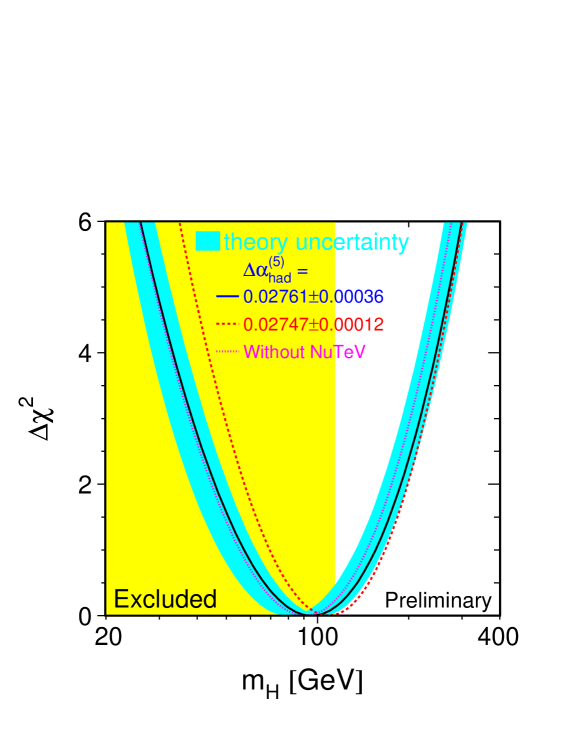
Figure 12: Of particular interest is the constraint on the mass $m_{h}$ of the Higgs boson, because this fundamental ingredient of the Standard Model has not been observed yet. The figure shows the $\Delta\chi^{2}=\chi^{2}-\chi^{2}_{min}$ vs. $m_{h}$ curve derived from precision electroweak measurements, assuming the Standard Model to be the correct theory of nature. The solid line is the result of the fit using all data while the band represents an estimate of the theoretical error due to missing higher order corrections. The vertical band shows the 95% CL exclusion limit on $m_{h}$ from the direct Higgs search at LEP. (From Ref. unknown:2003ih.)

6.4 Comparing the values for the electroweak observables

Once we have the best fit values for the floating parameters, we can predict the theoretical central values ${\mathcal{O}}^{th}$ for the remaining observables in Tables 1.1 and 1.2. We can then compare theory (${\mathcal{O}}^{th}$) to experiment (${\mathcal{O}}^{exp}$). The results are usually presented as “pulls”, which in Tables 1.1 and 1.2 are defined as

$${\rm pull}=\frac{{\mathcal{O}}^{th}-{\mathcal{O}}^{exp}}{\sigma^{th}},$$ (53)

where $\sigma^{th}$ is the error on ${\mathcal{O}}^{th}$.

All in all, the fit is successful, as evidenced from Fig. 13. One is tempted to conclude that the SM works pretty well, having been tested at the level of 1% and less. No major discrepancies are observed, and, with so many measurements, a few $2-3\sigma$ deviations are simply inevitable.

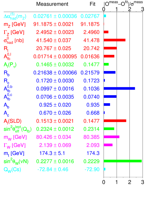
Figure 13: Agreement between the measured values for some of the precision electroweak observables and their SM predictions, as of the Summer of 2003. (From the LEP EWWG[19].)

6.5 The Higgs mass prediction

Let us now understand better where the Higgs mass prediction comes from. Ideally, we should concentrate on those observables which exhibit the strongest dependence on the Higgs boson mass $m_{h}$. For this purpose, it is useful to plot the theoretical prediction for each observable as a function of $m_{h}$ and contrast it with the experimental measurement (see Figures 14-17). We see that the observables most sensitive to $m_{h}$ are the $W$ mass $M_{W}$ and the asymmetries. We will discuss these in more detail in the next two subsections.

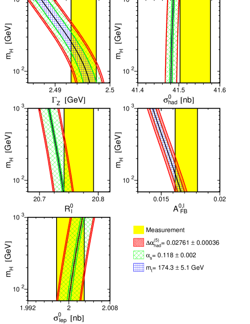
Figure 14: Comparison of LEP-I measurements with the SM prediction as a function of $m_{h}$. The measurement with its error is shown as the vertical band. The width of the SM band is due to the uncertainties in $\Delta\alpha_{had}^{(5)}(M_{Z})$, $\alpha_{s}(M_{Z})$ and $m_{t}$. The total width of the band is the linear sum of these effects. (From the LEP EWWG [20].)

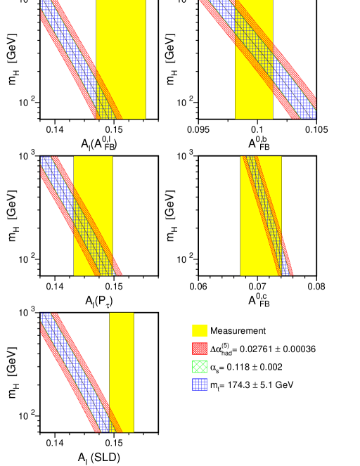
Figure 15: Comparison of LEP-I measurements with the SM prediction as a function of $m_{h}$. The measurement with its error is shown as the vertical band. The width of the SM band is due to the uncertainties in $\Delta\alpha_{had}^{(5)}(M_{Z})$, $\alpha_{s}(M_{Z})$ and $m_{t}$. The total width of the band is the linear sum of these effects. Also shown is the comparison of the SLD measurement of ${\mathcal{A}}_{\ell}$, dominated by $A^{0}_{LR}$, with the SM. (From the LEP EWWG [20].)

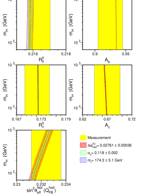
Figure 16: Comparison of LEP-I and SLD heavy flavor measurements with the SM prediction as a function of $m_{h}$. The measurement with its error is shown as the vertical band. The width of the SM band is due to the uncertainties in $\Delta\alpha_{had}^{(5)}(M_{Z})$, $\alpha_{s}(M_{Z})$ and $m_{t}$. The total width of the band is the linear sum of these effects. Also shown is the comparison of the LEP-I measurement of the inclusive hadronic charge asymmetry $Q^{had}_{FB}$ with the SM. (From the LEP EWWG [20].)

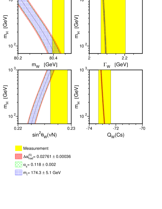
Figure 17: Comparison of $M_{W}$ and $\Gamma_{W}$ measured at LEP-II and $p\bar{p}$ colliders, of $\sin^{2}\theta_{W}$ measured by NuTeV and of atomic parity violation in caesium with the SM prediction as a function of $m_{h}$. The measurement with its error is shown as the vertical band. The width of the SM band is due to the uncertainties in $\Delta\alpha_{had}^{(5)}(M_{Z})$, $\alpha_{s}(M_{Z})$ and $m_{t}$. The total width of the band is the linear sum of these effects. (From the LEP EWWG [20].)

6.6 Impact of the $M_{W}$ measurement on $m_{h}$

An approximate formula for $M_{W}$ (in the $\overline{MS}$ scheme), which exhibits the dependence on the relevant electroweak parameters, is [34]

$$M_{W} = 80.3827-0.0579\ln\left(\frac{m_{h}}{100\ GeV}\right)-0.008\ln^{2}\left(\frac{m_{h}}{100\ GeV}\right)$$ (54)

$$- 0.517\left(\frac{\Delta\alpha_{had}^{(5)}(M_{Z})}{0.0280}-1\right)+0.543\left(\left(\frac{m_{t}}{175\ GeV}\right)^{2}-1\right)$$

$$- 0.085\left(\frac{\alpha_{s}(M_{Z})}{0.118}-1\right).$$

The experimentally measured value for $M_{W}$ seems to be a bit high (Table 1.2). As we can see from (54), a largish $M_{W}$ can be explained by either a small $m_{h}$, a larger $m_{t}$, a smaller $\alpha_{s}$, or some combination of the above. The correlation between $M_{W}$, $m_{t}$ and $m_{h}$ from the precision data is shown in Fig. 18, where the solid contour delineates the 68% CL region resulting from a global fit omitting the $M_{W}$, $\Gamma_{W}$ and $m_{t}$ measurements. Also shown is the SM prediction for this correlation, for $m_{h}=114,300,1000$ GeV. We first see that the indirect determination of $M_{W}$ and $m_{t}$ from precision data alone is in very good agreement with the direct $M_{W}$ and $m_{t}$ measurements shown with the dashed contour. This fact may not look that impressive, now that the top quark and the $W$ boson have been discovered, but nevertheless it should be considered as a triumphant success of the precision program. We also see that both the direct and indirect measurements of $M_{W}$ and $m_{t}$ prefer a light Higgs boson.

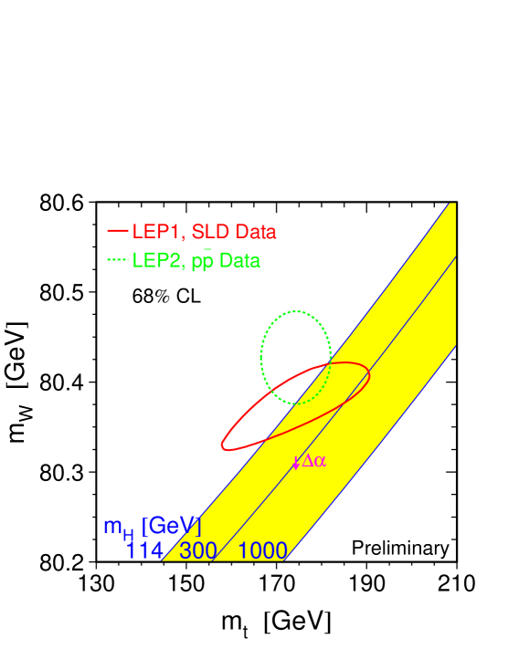
Figure 18: A comparison of the indirect measurements of $M_{W}$ and $m_{t}$ (LEP-I+SLD data) (solid contour) and the direct measurements ($p\bar{p}$ colliders and LEP-II data) (dashed contour). In both cases the 68% CL contours are plotted. Also shown is the SM relationship for the masses as a function of $m_{h}$. The arrow labelled $\Delta\alpha$ shows the variation of this relation if $\alpha(M_{Z})$ is changed by $1\sigma$. This variation leads to an additional uncertainty to the SM band shown in the figure. From Ref. unknown:2003ih.

6.7 Impact of the asymmetry measurements on $m_{h}$

The asymmetries (or equivalently, $\sin^{2}\theta_{eff}$) also exhibit significant sensitivity to $m_{h}$. Examining Figure 15, we notice a couple of things. First, $A_{\ell}$ and $A_{FB}^{b,c}$ place contradictory demands on the Higgs mass: $A_{\ell}$ prefers a very small $m_{h}$ while $A_{FB}^{b,c}$ prefer a heavier Higgs boson. There are a couple of $A_{\ell}$ measurements – one from LEP and the other from SLD, and they seem to be in agreement. Second, since the best fit value for $m_{h}$ is low, this means that $A_{FB}^{b,c}$ will be off from its “SM prediction”. Finally, the NuTeV measurement of $\sin^{2}\theta_{W}$ (Figure 17) also seems to prefer a rather heavy Higgs boson. The results for the various asymmetries are often conveniently summarized as measurements of $\sin^{2}\theta_{\rm eff}^{\rm lept}$ (Fig. 19).

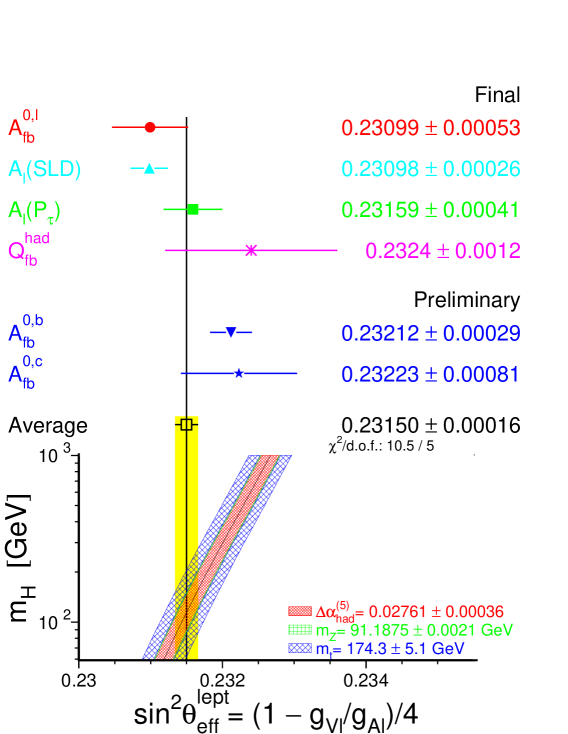
Figure 19: Comparison of several determinations of $\sin^{2}\theta_{\rm eff}^{\rm lept}$ from asymmetries. Also shown is the prediction of the SM as a function of $m_{h}$. The width of the SM band is due to the uncertainties in $\Delta\alpha_{had}^{(5)}(M_{Z})$, $M_{Z}$ and $m_{t}$. The total width of the band is the linear sum of these effects. (From Ref. unknown:2003ih.)

6.8 A Higgs puzzle?

Tables 1.1 and 1.2 contain a large number of observables, with different sensitivity to the Higgs mass $m_{h}$. Let us concentrate on a few selected observables with sufficient resolving power with respect to $m_{h}$ and look at the range of $m_{h}$ preferred by each one (Figure 20).

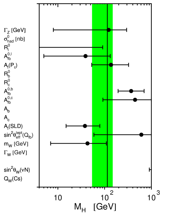
Figure 20: Preferred range for the SM Higgs mass $m_{h}$ from various electroweak observables. The shaded band denotes the overall constraint on the mass of the Higgs boson derived from the full data set. (From Ref. unknown:2003ih.)

We see that, as discussed previously, $M_{W}$ and the leptonic asymmetries prefer a very light Higgs boson, while $A_{FB}^{b,c}$ and NuTeV prefer a heavy Higgs boson. The current best fit value of $m_{h}$ of just below the LEP limit arises from the combination of these somewhat contradictory measurements. Is this a problem? Chanowitz has made the argument that this discrepancy presents a “no-lose” case for new physics [35, 36]:

• One possible interpretation is that $A_{FB}^{b,c}$ is already indicative of new physics, and the discrepancy is real. However, any such new physics effect should not contribute too much to $R_{b}$, which seems to be in agreement with the SM. Proposed solutions to the puzzle include a heavy $Z^{\prime}$ boson with nonuniversal couplings to the third family [37, 38, 39] and mirror vector-like fermions mixing with the $b_{R}$ quark [40].

• Alternatively, the $A_{FB}^{b,c}$ (and possibly the NuTeV) measurement could be wrong due to a statistical fluctuation or some unknown systematics. In that case, we should throw out the suspect measurements from the fit altogether. This significantly improves the goodness of fit, but at the expense of a much lower best fit value of $m_{h}$, whose upper bound from the fit becomes $m_{h}<120$ GeV at 95% CL, leading to some tension with the direct LEP bound $m_{h}>114$ GeV. In this scenario new physics is again needed in order to modify the radiative corrections and thus allow an acceptable $m_{h}$ [41, 42]. However, one should keep in mind that the tension between the indirect determination of $m_{h}$ and the direct lower bound from LEP is statistically rather weak at the moment, and may be alleviated significantly, if, for example, the top quark turned out to be a little heavier, as suggested by the recent D0 analysis of their Run I data [43] (which gives $m_{t}=180.1\pm 5.4$ GeV). This is illustrated in Figure 21, which shows the effect of a $1\sigma$ upward fluctuation in $m_{t}$ on the indirect Higgs mass determination [44].

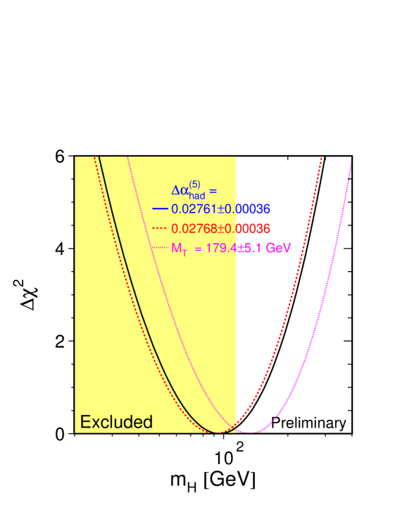
Figure 21: The effect of a $1\sigma$ change in $m_{t}$ on the Higgs mass constraints. (From Ref. Gambino:2003xc.)

7 Testing for New Physics

The precision data can be used to constrain or point towards new physics. To this end, there are different approaches.

• Model-independent. If there is new physics, then upon integrating out the new heavy degrees of freedom we will end up with a set of higher dimensional operators in the low-energy lagrangian. The most model-independent approach, therefore, will be to write down all possible higher-dimensional operators consistent with the symmetries of the Standard Model. These operators will be suppressed by some scale $\Lambda$ (presumably the scale where the new physics will appear) to the appropriate power. The size of these operators can be parameterized by dimensionless coefficients of order unity. We can then use the precision electroweak data in order to constrain the dimensionless coefficients of the relevant operators [45, 46, 47]. The advantage of this approach is that it is completely model-independent. Unfortunately it is too complicated and time-consuming, and is rarely used for the case of more than a few operators.

• Model-dependent. Alternatively, one can completely specify the new physics model of interest, e.g. minimal supergravity [48], minimal gauge mediation [48], minimal universal extra dimensions [49, 50], little Higgs models [51, 52, 53, 54, 55, 56], etc. One can then compute the contributions from new physics to the precision observables in terms of (41) supplemented by the new physics model parameters $\{q\}$:

  $${\mathcal{O}}_{i}^{theory}={\mathcal{O}}_{i}^{tree}(\alpha,G_{F},M_{Z})\left[1+\Delta_{i}^{SM}(\{p\})+\Delta_{i}^{NP}(\{p,q\})\right],$$ (55)

  redo the fits and derive best fit values and constraints on $\{q\}$ in a similar way as was done for $\{p\}$. In full generality (i.e. full leading order corrections to all precision observables), the method is again very time-consuming, so it is usually applied for a single (or a few) observables.

• Oblique parameters. A third method, which sits somewhere in between, is the method of the so called $S,T,U$ parameters (also called Peskin-Takeuchi parameters [57, 58]). It amounts to making the approximation that the dominant new physics effects reside in the gauge boson propagators (self-energies). Notice that almost every electroweak observable involves some gauge boson propagator. So once we compute the new physics effects on the gauge boson propagators, we have essentially accounted for a whole class of corrections which appear in every observable, i.e. they are universal. In this method one neglects the process-specific corrections, i.e. the vertex and box corrections and the fermion (and Higgs) self-energies. Apriori we don’t know whether this approximation is justified within a specific new physics model, however, there are many classes of models where it works. In scenarios with many new particles, there is a simple argument as to why the oblique corrections are most of the story - the gauge bosons couple to all particles charged under the corresponding gauge group, hence their self-energy corrections are enhanced by the multiplicity of the new particles. In contrast, the flavor of the loop particles in the process-specific corrections is fixed by the flavor on the external legs. To summarize, the advantages of the method are: 1) simple calculations (there aren’t too many relevant diagrams); 2) universality – i.e. the parameters are computed once and for all and affect all observables; 3) if $S,T,U$ are added as free parameters to (41), their best fit values can be computed ahead of time by the fitting experts, and then supplied to model-builders, who in turn only need to learn to calculate $S,T,U$ within a specific model and need not worry about the fitting procedure.

7.1 $S$, $T$, $U$ parameters

The $S,T,U$ parameters are defined as [2]

$$\widehat{\alpha}_{e}(M_{Z})T \equiv \frac{\Pi^{new}_{WW}(0)}{M_{W}^{2}}-\frac{\Pi^{new}_{ZZ}(0)}{M_{Z}^{2}},$$ (56)

$$\frac{\widehat{\alpha}_{e}(M_{Z})}{4\widehat{s}^{2}_{Z}\widehat{c}^{2}_{Z}}S \equiv \frac{\Pi^{new}_{ZZ}(M_{Z}^{2})-\Pi^{new}_{ZZ}(0)}{M_{Z}^{2}},$$ (57)

$$\frac{\widehat{\alpha}_{e}(M_{Z})}{4\widehat{s}^{2}_{Z}}(S+U) \equiv \frac{\Pi^{new}_{WW}(M_{W}^{2})-\Pi^{new}_{WW}(0)}{M_{W}^{2}}.$$ (58)

where $\widehat{s}_{Z}^{2}$ is defined in terms of the $\overline{MS}$ running couplings as $\widehat{s}_{Z}^{2}\equiv{\widehat{g}^{\prime}}{}^{2}(M_{Z})/(\widehat{g}^{\prime}{}^{2}(M_{Z})+\widehat{g}^{2}(M_{Z}))$. Notice that the $S,T,U$ parameters are defined so that for the Standard Model they are equal to 0.

One can now consider $S,T,U$ as floating parameters added to (41) and redo the fits to electroweak data. The current global fit result is [1]

$$S = -0.14\pm 0.10(-0.08),$$ (59)

$$T = -0.15\pm 0.12(+0.09),$$ (60)

$$U = +0.32\pm 0.12(+0.01)$$ (61)

for $m_{h}=115.6$ GeV (the parentheses show the change in going to $m_{h}=300$ GeV). Best fit contours in the $S-T$ plane (for $U=0$) are shown in Fig. 22.

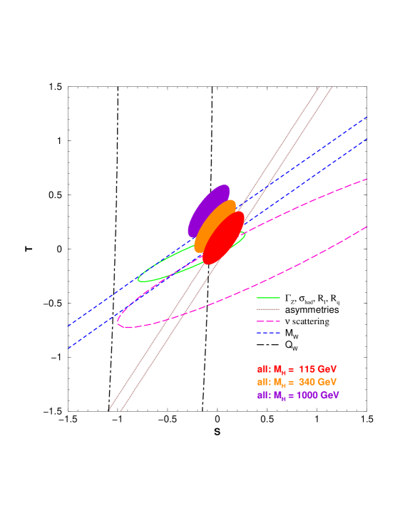
Figure 22: $1\sigma$ constraints on $S$ and $T$ from various inputs. The contours assume $m_{h}=115$ GeV except for the central and upper 90% CL regions (shaded, from all data) which are for $m_{h}=340$ GeV and $m_{h}=1000$ GeV, correspondingly. All fits assume $U=0$. (From Ref. Erler:ew.)

We see that $S=T=0$ is in the region of a light Higgs boson, i.e. in the absence of new physics, the fits prefer small $m_{h}$, as we saw in the previous Section. However, a heavy Higgs is not out of the question, provided there are positive new physics contributions to $T$.

7.2 Constraining new physics scenarios

Previously we saw that precision electroweak data generally prefers a light SM Higgs boson (Figure 12), in which case any new physics effects appearing through $S$, $T$ and $U$ should be small. However, this does not rule out a possible “conspiracy” [59, 60], where the undesired contributions from a heavy Higgs boson in the SM are fortuitously cancelled by new physics effects. While a “conspiracy” is still a valid option in principle, the current thinking is that it would involve a large degree of fine-tuning and is therefore theoretically disfavored. As a result, we tend to like new physics models where no major deviations in the precision observables are expected. A simple and effective way to guarantee this is to have the new physics contribute only at the loop level, for example due to a conserved symmetry which distinguishes the SM particles from the rest. Some well known examples are: supersymmetry with conserved $R$-parity, Universal Extra Dimensions with conserved $KK$-parity [49], and little Higgs models with conserved $T$-parity [61]. Conversely, models with tree-level contributions to electroweak observables (e.g. generic little Higgs theories) tend to have trouble with the data.

8 Concluding Remarks

Overall, the SM is in good shape, and the agreement between theory and experiment has in fact improved since the time of TASI-2002. The results in Tables 1.1 and 1.2 are from 1/03 [1], while the electroweak data shown at the TASI school was from 7/01 [16]. Some notable changes and recent updates are the following:

• Table 1.2 lists the Summer 2002 value for $M_{W}$ ($80.447\pm 0.042$ GeV), but in the Winter of 2003 a revised ALEPH analysis lowered the LEP average to $80.412\pm 0.042$ GeV, which is closer to the SM best fit prediction and will lead to a small increase in the best fit value for $m_{h}$.

• New measurements of $M_{W}$ and $m_{t}$ are expected soon from Run II at the Tevatron. A new preliminary DO analysis [43] of Run I data gives $m_{t}=180.1\pm 5.4$ GeV, which again will raise the best fit value for $m_{h}$.

• The NuTeV results on deep inelastic scattering in terms of $\sin^{2}\theta_{W}$ ($0.2277\pm 0.0016$) are $3.0\sigma$ above the global fit value of $0.2228\pm 0.0004$. Possible explanations of the NuTeV anomaly include an unexpectedly large violation of isospin in the quark sea [62, 63], the effect of an asymmetric strange sea [62, 63, 64], nuclear shadowing [65, 66] or NLO QCD corrections [67, 68].

• The status of the $g_{\mu}-2$ anomaly after the 2002 result from BNL was still somewhat uncertain, depending on the particular theoretical analysis used to extract the hadronic contribution to the Standard Model prediction for $g_{\mu}-2$. In addition, last year the CMD-2 Collaboration at Novosibirsk discovered that part of the radiative treatment was incorrectly applied to their $e^{+}e^{-}$ data (a lepton vacuum polarization diagram was omitted) which prompted a reanalysis of the $e^{+}e^{-}$ data [69]. This subsequently brought the theory prediction in better agreement with experiment: the deviation was $1.9\sigma$ ($0.7\sigma$) for the $e^{+}e^{-}$ ($\tau$-based) estimates [70, 71]. The final result based on negative muons has just been announced [72]. It is consistent with the previous measurements and brings the world average to $a_{\mu}(exp)=11659208(6)\times 10^{-10}$ (0.5 ppm). The difference between $a_{\mu}(exp)$ and the SM theoretical prediction based on the $e^{+}e^{-}$ or $\tau$ data is now $2.7\sigma$ and $1.4\sigma$, respectively. New results from KLOE and BABAR may help sort out the theoretical predictions. If the discrepancy stands, an obvious candidate for a new physics explanation would be supersymmetry with relatively low superpartner masses and large $\tan\beta$ [73, 74].

References

- [1] P. Langacker, “Electroweak physics,” arXiv:hep-ph/0308145.
- [2] J. Erler and P. Langacker, “Electroweak Model And Constraints On New Physics (Rev.),” Phys. Rev. D 66, 010001 (2002).
- [3] K. Hagiwara et al. [Particle Data Group Collaboration], “Review Of Particle Physics,” Phys. Rev. D 66, 010001 (2002).
- [4] A. Pich, “The Standard model of electroweak interactions,” arXiv:hep-ph/9412274.
- [5] P. Langacker, “Precision electroweak measurements,” Prepared for Theoretical Advanced Study Institute in Elementary Particle Physics (TASI 95): QCD and Beyond, Boulder, Colorado, 4-30 Jun 1995.
- [6] D. M. Pierce, “Renormalization of supersymmetric theories,” arXiv:hep-ph/9805497.
- [7] J. L. Hewett, “The standard model and why we believe it,” arXiv:hep-ph/9810316.
- [8] S. Dawson, “Introduction to electroweak symmetry breaking,” arXiv:hep-ph/9901280.
- [9] Y. K. Kim, “Precision electroweak physics,” Prepared for Theoretical Advanced Study Institute in Elementary Particle Physics (TASI 2000): Flavor Physics for the Millennium, Boulder, Colorado, 4-30 Jun 2000.
- [10] J. Drees, Int. J. Mod. Phys. A 17, 3259 (2002) [arXiv:hep-ex/0110077].
- [11] P. B. Renton, Rept. Prog. Phys. 65, 1271 (2002) [arXiv:hep-ph/0206231].
- [12] P. Langacker, “Precision Tests Of The Standard Electroweak Model,” (Advanced series on directions in high energy physics, v. 14), Singapore, World Scientific (1995) 1008 p.
- [13] T. L. . Barklow, S. Dawson, H. E. . Haber and J. L. . Siegrist, “Electroweak Symmetry Breaking And New Physics At The Tev Scale,” (Advanced series on directions in high energy physics, v. 16), Singapore, World Scientific (1996) 736 p.
- [14] M. G. Green, S. L. Lloyd, P. N. Ratoff and D. R. Ward, “Electron-Positron Physics at the ,” (Studies in High Energy Physics Cosmology and Gravitation), Bristol and Philadelphia, IoP Publishing (1998) 383 p.
- [15] R. Brock et al., “Report of the working group on precision measurements,” arXiv:hep-ex/0011009.
- [16] P. Langacker, “Precision electroweak data: Phenomenological analysis,” in Proc. of the APS/DPF/DPB Summer Study on the Future of Particle Physics (Snowmass 2001) ed. N. Graf, eConf C010630, P107 (2001) [arXiv:hep-ph/0110129].
- [17] U. Baur, R. Clare, J. Erler, S. Heinemeyer, D. Wackeroth, G. Weiglein and D. R. Wood, “Theoretical and experimental status of the indirect Higgs boson mass determination in the standard model,” in Proc. of the APS/DPF/DPB Summer Study on the Future of Particle Physics (Snowmass 2001) ed. N. Graf, eConf C010630, P122 (2001) [arXiv:hep-ph/0111314].
- [18] U. Baur et al. [The Snowmass Working Group on Precision Electroweak Measurements Collaboration], “Present and future electroweak precision measurements and the indirect determination of the mass of the Higgs boson,” in Proc. of the APS/DPF/DPB Summer Study on the Future of Particle Physics (Snowmass 2001) ed. N. Graf, eConf C010630, P1WG1 (2001) [arXiv:hep-ph/0202001].
- [19] See the website of the LEP Electroweak Working Group at http://lepewwg.web.cern.ch/LEPEWWG/
- [20] LEP Collaboration, “A combination of preliminary electroweak measurements and constraints on the standard model,” arXiv:hep-ex/0312023.
-
[21]
The document
“Facilities for the Future of Science: A Twenty-Year Outlook”, is available at
http://www.sc.doe.gov/. - [22] G. Montagna, O. Nicrosini and F. Piccinini, Riv. Nuovo Cim. 21N9, 1 (1998) [arXiv:hep-ph/9802302].
- [23] D. Buskulic et al. [ALEPH Collaboration], Z. Phys. C 60, 71 (1993).
- [24] G. Altarelli, R. Kleiss and C. Verzegnassi, “Z Physics At Lep-1. Proceedings, Workshop, Geneva, Switzerland, September 4-5, 1989. Vol. 1: Standard Physics”.
- [25] M. Davier, L. Duflot, F. Le Diberder and A. Rouge, Phys. Lett. B 306, 411 (1993).
- [26] G. Abbiendi et al. [OPAL Collaboration], Eur. Phys. J. C 21, 1 (2001) [arXiv:hep-ex/0103045].
- [27] A. Heister et al. [ALEPH Collaboration], Eur. Phys. J. C 20, 401 (2001) [arXiv:hep-ex/0104038].
- [28] D. Chakraborty, J. Konigsberg and D. Rainwater, “Review of top quark physics,” arXiv:hep-ph/0303092.
- [29] W. Wagner [CDF Collaboration], “Top quark cross-section measurements at the Tevatron,” arXiv:hep-ex/0312008.
- [30] [CDF Collaboration], “Combination of CDF and D0 results on W boson mass and width,” arXiv:hep-ex/0311039.
- [31] V. M. Abazov et al. [D0 Collaboration], Phys. Rev. D 66, 032008 (2002) [arXiv:hep-ex/0204009].
- [32] D. Y. Bardin, P. Christova, M. Jack, L. Kalinovskaya, A. Olchevski, S. Riemann and T. Riemann, Comput. Phys. Commun. 133, 229 (2001) [arXiv:hep-ph/9908433].
- [33] J. Erler, “Global fits to electroweak data using GAPP,” arXiv:hep-ph/0005084.
- [34] A. Sirlin, “Ten years of precision electroweak physics,” in Proc. of the 19th Intl. Symp. on Photon and Lepton Interactions at High Energy LP99 ed. J.A. Jaros and M.E. Peskin, Int. J. Mod. Phys. A 15S1, 398 (2000) [eConf C990809, 398 (2000)] [arXiv:hep-ph/9912227].
- [35] M. S. Chanowitz, Phys. Rev. Lett. 87, 231802 (2001) [arXiv:hep-ph/0104024].
- [36] M. S. Chanowitz, Phys. Rev. D 66, 073002 (2002) [arXiv:hep-ph/0207123].
- [37] J. Erler and P. Langacker, Phys. Rev. Lett. 84, 212 (2000) [arXiv:hep-ph/9910315].
- [38] X. G. He and G. Valencia, Phys. Rev. D 66, 013004 (2002) [Erratum-ibid. D 66, 079901 (2002)] [arXiv:hep-ph/0203036].
- [39] X. G. He and G. Valencia, Phys. Rev. D 68, 033011 (2003) [arXiv:hep-ph/0304215].
- [40] D. Choudhury, T. M. P. Tait and C. E. M. Wagner, Phys. Rev. D 65, 053002 (2002) [arXiv:hep-ph/0109097].
- [41] G. Altarelli, F. Caravaglios, G. F. Giudice, P. Gambino and G. Ridolfi, JHEP 0106, 018 (2001) [arXiv:hep-ph/0106029].
- [42] A. Datta and A. Datta, Phys. Lett. B 578, 165 (2004) [arXiv:hep-ph/0210218].
- [43] P. Azzi, “Top quark measurements at the Fermilab Tevatron,” arXiv:hep-ex/0312052.
- [44] P. Gambino, “The top priority: Precision electroweak physics from low to high energy,” arXiv:hep-ph/0311257.
- [45] F. Feruglio, Int. J. Mod. Phys. A 8, 4937 (1993) [arXiv:hep-ph/9301281].
- [46] T. Appelquist and G. H. Wu, Phys. Rev. D 48, 3235 (1993) [arXiv:hep-ph/9304240].
- [47] J. Wudka, Int. J. Mod. Phys. A 9, 2301 (1994) [arXiv:hep-ph/9406205].
- [48] J. Erler and D. M. Pierce, Nucl. Phys. B 526, 53 (1998) [arXiv:hep-ph/9801238].
- [49] T. Appelquist, H. C. Cheng and B. A. Dobrescu, Phys. Rev. D 64, 035002 (2001) [arXiv:hep-ph/0012100].
- [50] T. Appelquist and H. U. Yee, Phys. Rev. D 67, 055002 (2003) [arXiv:hep-ph/0211023].
- [51] C. Csaki, J. Hubisz, G. D. Kribs, P. Meade and J. Terning, Phys. Rev. D 67, 115002 (2003) [arXiv:hep-ph/0211124].
- [52] J. L. Hewett, F. J. Petriello and T. G. Rizzo, JHEP 0310, 062 (2003) [arXiv:hep-ph/0211218].
- [53] C. Csaki, J. Hubisz, G. D. Kribs, P. Meade and J. Terning, Phys. Rev. D 68, 035009 (2003) [arXiv:hep-ph/0303236].
- [54] T. Gregoire, D. R. Smith and J. G. Wacker, “What precision electroweak physics says about the SU(6)/Sp(6) little Higgs,” arXiv:hep-ph/0305275.
- [55] R. Casalbuoni, A. Deandrea and M. Oertel, “Little Higgs models and precision electroweak data,” arXiv:hep-ph/0311038.
- [56] C. Kilic and R. Mahbubani, “Precision electroweak observables in the minimal moose little Higgs model,” arXiv:hep-ph/0312053.
- [57] M. E. Peskin and T. Takeuchi, Phys. Rev. Lett. 65, 964 (1990).
- [58] M. E. Peskin and T. Takeuchi, Phys. Rev. D 46, 381 (1992).
- [59] C. F. Kolda and H. Murayama, JHEP 0007, 035 (2000) [arXiv:hep-ph/0003170].
- [60] M. E. Peskin and J. D. Wells, Phys. Rev. D 64, 093003 (2001) [arXiv:hep-ph/0101342].
- [61] H. C. Cheng and I. Low, JHEP 0309, 051 (2003) [arXiv:hep-ph/0308199].
- [62] S. Davidson, S. Forte, P. Gambino, N. Rius and A. Strumia, JHEP 0202, 037 (2002) [arXiv:hep-ph/0112302].
- [63] G. P. Zeller et al. [NuTeV Collaboration], Phys. Rev. D 65, 111103 (2002) [Erratum-ibid. D 67, 119902 (2003)] [arXiv:hep-ex/0203004].
- [64] R. H. Bernstein [NuTeV Collaboration], J. Phys. G 29, 1919 (2003) [arXiv:hep-ex/0210061].
- [65] G. A. Miller and A. W. Thomas, “Comment on ’A precise determination of electroweak parameters in neutrino-nucleon scattering’,” arXiv:hep-ex/0204007.
- [66] W. Melnitchouk and A. W. Thomas, Phys. Rev. C 67, 038201 (2003) [arXiv:hep-ex/0208016].
- [67] B. A. Dobrescu and R. K. Ellis, “Analytic estimates of the QCD corrections to neutrino nucleus scattering,” arXiv:hep-ph/0310154.
- [68] S. Kretzer, F. Olness, J. Pumplin, D. Stump, W. K. Tung and M. H. Reno, “The parton structure of the nucleon and precision determination of the Weinberg angle in neutrino scattering,” arXiv:hep-ph/0312322.
- [69] R. R. Akhmetshin et al. [CMD-2 Collaboration], Phys. Lett. B 578, 285 (2004) [arXiv:hep-ex/0308008].
- [70] M. Davier, S. Eidelman, A. Hocker and Z. Zhang, Eur. Phys. J. C 31, 503 (2003) [arXiv:hep-ph/0308213].
- [71] K. Hagiwara, A. D. Martin, D. Nomura and T. Teubner, “Predictions for g-2 of the muon and ,” arXiv:hep-ph/0312250.
- [72] G. W. Bennett [Muon g-2 Collaboration], “Measurement of the negative muon anomalous magnetic moment to 0.7-ppm,” arXiv:hep-ex/0401008.
- [73] J. L. Feng and K. T. Matchev, Phys. Rev. Lett. 86, 3480 (2001) [arXiv:hep-ph/0102146].
- [74] L. L. Everett, G. L. Kane, S. Rigolin and L. T. Wang, Phys. Rev. Lett. 86, 3484 (2001) [arXiv:hep-ph/0102145].